Modelling study of the impact of deep convection on the UTLS air composition – Part II: Ozone budget in the TTL avenue de la Recherche Scientifique, 45071 Orléans cedex 2, France

(1)

HAL Id: hal-00327974

https://hal.archives-ouvertes.fr/hal-00327974

Submitted on 23 Sep 2005

HAL is a multi-disciplinary open access

archive for the deposit and dissemination of sci-entific research documents, whether they are pub-lished or not. The documents may come from teaching and research institutions in France or abroad, or from public or private research centers.

L’archive ouverte pluridisciplinaire HAL, est destinée au dépôt et à la diffusion de documents scientifiques de niveau recherche, publiés ou non, émanant des établissements d’enseignement et de recherche français ou étrangers, des laboratoires publics ou privés.

Modelling study of the impact of deep convection on the

UTLS air composition – Part II: Ozone budget in the

TTL avenue de la Recherche Scientifique, 45071 Orléans

cedex 2, France

E. D. Rivière, V. Marécal, N. Larsen, S. Cautenet

To cite this version:

E. D. Rivière, V. Marécal, N. Larsen, S. Cautenet. Modelling study of the impact of deep convection on the UTLS air composition – Part II: Ozone budget in the TTL avenue de la Recherche Scien-tifique, 45071 Orléans cedex 2, France. Atmospheric Chemistry and Physics Discussions, European Geosciences Union, 2005, 5 (5), pp.9169-9205. �hal-00327974�

(2)

ACPD

5, 9169–9205, 2005

Modelling study of the impact of deep convection on the UTLS air composition

– Part II

E. D. Rivi `ere et al.

Title Page Abstract Introduction Conclusions References Tables Figures J I J I Back Close Full Screen / Esc

Print Version

Interactive Discussion

Atmos. Chem. Phys. Discuss., 5, 9169–9205, 2005 www.atmos-chem-phys.org/acpd/5/9169/

SRef-ID: 1680-7375/acpd/2005-5-9169 European Geosciences Union

Atmospheric Chemistry and Physics Discussions

Modelling study of the impact of deep

convection on the UTLS air composition

– Part II: Ozone budget in the TTL

E. D. Rivi `ere1, V. Mar ´ecal1, N. Larsen2, and S. Cautenet3

1

Laboratoire de Physique et Chimie de l’Environnement/CNRS and Universit é d’Orl éans, 3A avenue de la Recherche Scientifique, 45071 Orl éans cedex 2, France

2

Danish Meteorological Institute, Division of Middle Atmosphere Research, Lyngbyvej 100, DK-2100, Copenhagen, Denmark

3

Laboratoire de M ét éorologie Physique/CNRS-OPGC/Universit é Blaise Pascal, 24 Avenue des Landais, 63177 Aubi ère cedex, France

Received: 29 March 2005 – Accepted: 2 May 2005 – Published: 23 September 2005 Correspondence to: V. Mar ´ecal (vmarecal@cnrs-orleans.fr)

(3)

ACPD

5, 9169–9205, 2005

– Part II

Print Version

Abstract

In this second part of a series of two papers which aim to study the local impact of deep convection on the chemical composition of the Upper Troposphere and Lower Stratosphere (UTLS), we focus on ozone simulation results using a mesoscale model that includes on-line chemistry. A severe convective system observed on 8 February

5

2001 at Bauru, Brazil, is studied. We show that there is an increase in the ozone con-centration in the tropical transitional layer (TTL) in the model during this event, which is compatible with ozone sonde observations from Bauru during the 2004 convective season. The model horizontal variability of ozone in this layer is comparable with the variability of the ozone sonde observations in the same area. The calculation of the

10

ozone budget in the TTL shows that the ozone behaviour in this layer is mainly driven by dynamics. The upward motions at the bottom of the TTL, related to the convection activity is the main contributor to the budget since it can explain 75% of the total ozone increase in the TTL, while the chemical ozone production inside the TTL is estimated to be 23.5% of the ozone increase if NO_xproduction by lightning (LNO_x) is taken into

ac-15

count. It is shown that downward motions at the tropopause induced by gravity waves generated by deep convection are non negligible in the TTL ozone budget, since it represents 11% of the ozone increase. The correlation between the convection activity and the vertical flux at 13 km, the vertical flux at 17 km, and the chemical production is brought to the fore in this simulation.

20

1. Introduction

It is now well accepted that deep convection plays an important role in the redistri-bution of chemical species from the boundary layer up to the upper troposphere (e.g. Dickerson et al., 1987; Thornton et al., 1997; Wang and Prinn, 2000). Some of the species transported to a few kilometres below the tropopause might be important for

25

(4)

ACPD

5, 9169–9205, 2005

– Part II

Print Version

CO, HO_x), and for its destruction in the stratosphere (e.g. Cl_y, Br_y, NO_x). The main way for species to reach the stratosphere is to cross the tropical tropopause (Holton et al., 1995), or possibly to cross laterally the extratropical tropopause (e.g. Ray et al., 1999; Schoeberl, 2004). Knowing the chemistry and composition of the layer below the tropical tropopause, called the tropical transitional layer (TTL), is a necessary step in

5

determinining the amount of each chemical compound entering the stratosphere. Once in the tropical stratosphere, all chemical compounds will be transported by the general Brewer-Dobson circulation to higher latitudes (Brewer, 1949), potentially affecting the global ozone budget.

Many chemical species (O₃, NO_x, HO_x, other ozone precursors, halogen species

10

including very short life substances) need to be studied throughout the whole tropo-sphere to better understand the TTL chemical composition. Among these species ozone is of specific interest for several reasons. Firstly, its behaviour in the TTL is not fully understood. From several balloon-borne ozone observations, it has been shown that the TTL is characterised by an increase of ozone with altitude (measurements

15

published in Taupin et al., 1999; Pundt et al., 2002; V ¨omel et al., 2002; Thompson et al., 2003) that extends in the stratosphere. On one hand, using climatological pro-files, Folkins et al. (2002) highlighted a typical “S-shaped” vertical profile of ozone in the tropical troposphere (consisting of an increase in the lower troposphere, a slight decrease in the middle troposphere and an increase in the upper troposphere), and

20

explained this tendency with a simple 1-D model. This model only takes into account the contributions of advection, convection, and chemical ozone production. Since the tropospheric processes taken into account in the model of Folkins et al. (2002) are enough to describe the climatological shape of the tropospheric ozone profile, it can be concluded that the increase of ozone in the TTL is not due to stratospheric production

25

of ozone.

On the other hand, on an individual measurement approach during the wet season (V ¨omel et al, 2002; Pundt et al., 2002; Dessler et al., 2002), the behaviour of O₃ in the TTL can be less regular and can lead to a local bulge or a sharp increase in the

(5)

ACPD

5, 9169–9205, 2005

– Part II

Print Version

vertical profile. This behaviour has not been fully explained yet, even though V ¨omel et al. (2002) explained one of these events with a passing Kelvin wave.

Secondly, considering the lifetime of ozone in the upper troposphere and the lower stratosphere (UTLS) due to chemical loss alone (typically longer than a month), the O₃ concentration is then determined by transport and chemical production (WMO, 2003).

5

While not a perfect tracer, this property makes ozone a relatively good indicator of vertical transport from the surface up to the TTL. On this basis Dessler et al. (2002) combined O₃with CO measurements, and Folkins et al. (2002) used an O₃ profile to infer the level of convective outflow.

Finally, ozone is one of the most measured species in the tropical upper troposphere.

10

This is helpful for conducting chemistry studies in the upper troposphere, even if the ozone chemistry is relatively complex.

In this context, the aim of this series of two papers is to study the chemical composi-tion of the UTLS associated with a deep convective event over Brazil. For this purpose, we are using simulations performed with a mesoscale model coupled on-line with a

15

chemistry model. The case studied here is the case observed on 8 February 2001 in the region of Bauru, State of S ˜ao Paulo, in the frame of the preparation campaign of the EC funded HIBISCUS project. The aim of HIBISCUS is to study the impact of the tropical region on ozone on a global scale. The first paper of the series (Mar ´ecal et al., 2005) is devoted to the description of the event, the validation of the

meteorolog-20

ical simulation results, and the study of the ozone precursor distribution in the UTLS associated with this severe event. This paper reports the following results. The CO re-sults are compatible with the airborne measurements previously performed over Brazil in another year during the convective season in the upper troposphere, and are also compatible with the MOPITT satellite monthly average data for February 2001. The

25

NO_xsimulation, taking into account a parameterisation of NO_xproduction by lightning, shows that this process strongly affects the NO_x distribution in the layer at 6–16 km, with a maximum mean value of 2 ppbv at 12.5 km in the area of convection. Local max-ima in the Non-Methane volatile organic compounds (VOCs) were also computed by

(6)

ACPD

5, 9169–9205, 2005

– Part II

Print Version

the model and were in the altitude range 8 to 12 km for propene and isoprene, and in the altitude range 7–15 km for formaldehyde and ethane. These relatively large values of Non-Methane VOCs in the upper troposphere, mainly due to vertical transport by deep convection, might affect the ozone budget in the TTL.

The aim of this second paper is to study the impact of deep convection on the ozone

5

behaviour in the UTLS with particular attention paid to its budget in the TTL. This analysis is based on the same short time and local scale simulation as in Mar ´ecal et al. (2005). In particular, we want to answer the following questions:

Is the model able to reproduce typical TTL ozone behaviour? What is the relative contribution of the dynamics and of the chemical processes to the upper tropospheric

10

O₃ distribution? What is the relative contribution of horizontal and vertical dynamics? Does the NO_x production by lightning directly affect the ozone concentration in the TTL?

In Sect. 2, we present the simulation results for ozone. Section 3 discusses the vali-dation of the ozone results using measured profiles published in the literature and DMI

15

O₃ sonde measurements performed from Bauru during the HIBISCUS field campaign in 2004. Section 4 is devoted to the estimation of the impact of the chemical ozone production on ozone in the TTL, while Sect. 5 discusses the dynamical and chemical budget of ozone in this layer. The main conclusions and perspectives of this paper are given in Sect. 6.

20

2. Ozone simulation results

2.1. Simulation summary

Since the model and the simulation setup are fully described in Mar ´ecal et al. (2005), we just briefly summarise the characteristics of the simulation in the present paper. The model used is the RAMS mesoscale model (Pielke et al., 1992; Cotton et al., 2003)

25

(7)

ACPD

5, 9169–9205, 2005

– Part II

Print Version

et al. (1996). The coupled model will be referred to hereafter as the RAMS-chemistry model (e.g. Taghavi et al., 2004). The chemical package of the RAMS-chemistry model takes account of 29 species with 72 gas phase reactions. Aqueous phase chemistry for 9 species is included. The model accounts for the NO_x production by lightning (LNO_x) using the parameterisation of Pickering et al. (1998) and references therein.

5

The initialisation of the chemical species is deduced from the chemistry transport model MOCAGE (Peuch et al., 1999). A 42-h simulation has been used, starting from 7 February 2001, 12:00 UT. The run is performed using two nested grids. The fine grid (referred later as Grid 2) has a horizontal grid spacing of 4 km×4 km and a vertical resolution of 0.5 km in the UTLS, covering 628 km×608 km, including the Bauru and

10

S ˜ao Paulo areas. The maximum convective activity in the model is reached at 22:00 UT on 8 February. Two simulations with different chemistry were performed. The first one, referred to as the “reference simulation”, includes NO_x production by lightning, except during the 12 first hours of the simulation. The spin-up period, that is, the initial period needed by the model to reach equilibrium, is evaluated to be 12 h. In order to avoid

15

unrealistic NO_xproduction by lightning, the LNO_xparameterisation has been switched-off during this period for the “reference” run. The other run, referred to hereafter as the “no LNO_x” simulation, does not take into account NO_x production by lightning.

2.2. Vertical structure

The evolution of the mean ozone profile in Grid 2 between 8 February 00:00 UT and

20

9 February 04:00 UT at 4 h increments, corresponding to the “reference” simulation, is shown in Fig. 1. The results of the “no LNO_xsimulation” are also plotted for two specific times. The corresponding standard deviations normalised by the average values are plotted in Fig. 2. For each profile, we can broadly distinguish 3 different layers. The first layer, in the altitude range 8 to 13 km is characterised by an almost constant value

25

with altitude (∼40 ppbv) and a relatively weak change with time. The corresponding variability is relatively low (typically about 12%), with values increasing with altitude. The second layer, from 13 km altitude up to the tropopause (∼17 km in our case)

(8)

cor-ACPD

5, 9169–9205, 2005

– Part II

Print Version

responds to the beginning of the O₃ mixing ratio increase with altitude, even for the initial time profile. This behaviour is typical of the TTL and the range of this second layer matches well the altitude range given by the several definitions of the TTL. Thus in the following, we will call the layer between 13 km and the tropopause the TTL. In the simulations, the TTL exhibits an important evolution of O₃with time. In this layer,

5

relatively high values of the standard deviation are found. However, different shapes of the variability profile are found depending on time. The third layer, lying above 17 km, corresponds to the stratosphere and is characterised by an ozone increase with alti-tude and a very weak time evolution. The variability in the stratosphere is much lower than in the TTL, with values typically below 10%. It tends to decrease with altitude.

10

2.3. Time evolution

In the first layer (8 to 13 km), the changes of ozone with time are weak. In the after-noon of 8 February 2001, an increase of ozone is found in the model. Concurrently, a decrease of ozone is found after sunset. These features might be related to the O₃ production cycle in the presence of ozone precursors. Mar ´ecal et al. (2005) have

15

shown that convective activity brings large amounts of ozone precursors to the upper troposphere. Therefore, ozone is chemically produced during daytime while sunset corresponds to the time when ozone is chemically destroyed. The dynamics might also play a role in this time evolution. Particularly, the ozone variability increases with time and is likely due to the enhancement of the convection activity with time. Both

20

dynamical and chemical effects will be further analysed in Sects. 4 and 5.

The TTL exhibits the most significant variation with time during the convective event. It is worth noting that a comparison of the initial state (solid black line) and the profile 12 h later (solid green line) shows that there is no significant difference in the mean profile over this period (Fig. 1). This is correlated with a weak convective activity in both

25

the model and the observations from the Bauru radar. The variability for 7 February, 12:00 UT and for 8 February, 00:00 UT is also similar, differing by only 3 percentage points at the most. These differences are probably due to dynamical processes. The

(9)

ACPD

5, 9169–9205, 2005

– Part II

Print Version

mean profile for 8 February at 04:00 UT is not significantly different from the initial state, even though there is a slight increase in ozone in the layer range 15–17 km.

From this time there is a continuous increase in the mean ozone mixing ratio in the TTL, reaching a maximum on 9 February at 04:00 UT. The increase between 8 February, 20:00 UT and 9 February 04:00 UT is greater than for other time intervals,

5

while there is only a slight increase between 16:00 and 20:00 UT on 8 February 2001. The time increase in the ozone amount in the TTL leads to a specific shape in the vertical ozone profile for 9 February at 04:00 UT. This disturbed behaviour in the TTL is characterised by a local inflection in the increase of ozone, which is different from the initial profile for which the derivative of ozone with respect to altitude was monotonic.

10

In the TTL, the variability tendency starts with a decrease with time (until 8 February at 04:00 UT) followed by an increase until 8 February 16:00 UT. Between 16:00 UT and 20:00 UT, the variability is roughly constant with altitude in the TTL, oscillating vertically around a 17% value. For 9 February at 00:00 UT and 04:00 UT, the TTL variability exhibits a specific behaviour with two local maxima at 14 km (21%) and 16.8 km (18%)

15

and a local minimum in the middle of it (about 10% at 14.8 km). This could indicate that the evolution of the ozone in the TTL is driven by two different processes at the top and at the bottom of it.

In the lower stratosphere, the mean profile remains unchanged with time up to 20 km. The corresponding variability, which decreases with altitude, does not evolve

signifi-20

cantly with time. Above this level, there is a slight increase on mean ozone and corre-sponding variability with time from 16:00 UT on 8 February.

Two mean profiles (variability, respectively) corresponding to the “no LNO_x simula-tion” are also plotted in Fig. 1 (Fig. 2, respectively). 8 February at 08:00 UT is the latest time for which no differences appear between the profiles from the “reference” and “no

25

LNO_x” simulations. On 9 February at 00:00 UT, the differences in the mean and variabil-ity profiles between the simulations with and without LNO_xare large. These differences occurred in the range 9.5–14 km. This layer corresponds to the layer of the maximum of NO_x produced by lightning (see Fig. 7 in Mar ´ecal et al., 2005). On average, the

(10)

ACPD

5, 9169–9205, 2005

– Part II

Print Version

enhancement of ozone due to LNO_xreaches 8% in this layer. This result is consistent with the tendency given previously by the modelling studies of Jourdain (2003) and Labrador et al. (2004) that were based on a different approach. Using a global scale chemistry transport model which was run for a one year period, Labrador et al. (2004) estimated the tropospheric burden of O₃enhancement due to LNO_xto be 14%.

Jour-5

dain (2003) using a global circulation model which was run to give a simulation for one month, estimated the contribution of LNO_x to the O₃ enhancement over Brazil for the month of January to be 10 to 15%.

For any other altitude than [9.5 km, 14 km], including the disturbed layer of the TTL, the simulations with and without LNO_x superimpose in Fig. 1. This means that the

10

large increase of ozone in the TTL is not due entirely to the chemistry associated with enhanced NO_xfrom lightning. However, this does not rule out the potential role of the chemistry in producing the increase of O₃ for this layer since it has been shown in Mar ´ecal et al. (2005) that ozone precursors were present in this range of altitude, even in the “no LNO_x” simulation.

15

In order to evaluate the validity of the simulation, we compare the results with mea-surements performed in Brazil during the convective season in the next section.

3. Evaluation of the model results

Since no ozone sonde or balloon-borne measurements were available in the Bauru area during the simulation period, we have used for comparison, profiles from ozone

20

sondes launched from Bauru during February 2004. In our analysis, ozone sondes were preferred to balloon-borne remote sensing measurements because the latter type of instrument uses lines of sight of several hundred kilometres for profile retrieval, which induces a horizontal resolution that is coarser than the scale of a convective system. Since our aim is to study the impact of convection on the chemical distribution on a

25

(11)

ACPD

5, 9169–9205, 2005

– Part II

Print Version

3.1. DMI Ozone measurements

In the context of the HIBISCUS 2004 campaign, ozone sondes were launched regularly from Bauru between 10 and 24 February 2004. Standard electrochemical concentra-tion cells (ECC) ozone sondes were applied, using 3 ml. 1% KI-cathode soluconcentra-tions, with an estimated ozone measurement accuracy of about 5% (Komhyr et al., 1995).

5

A total of 10 profiles were obtained from the ground up to 26–27 km. They depict a wide range of different meteorological situations with respect to convection (close to or far from the convection, after or before a convective event). Thus, this set of mea-surements should help in evaluating our simulation, since inside the RAMS Grid 2 for a specific time, a wide range of situations with respect to the convection activity is also

10

encountered. The 10 ozone profiles are shown in Fig. 3 for the vertical range 8 km to 26 km. To provide a comparison with the RAMS-chemistry results, the simulated pro-files for the “reference” run for 7 February at 12:00 UT (initial time) and for 9 February at 00:00 UT are also shown. The mean profile from all the measurements was calcu-lated and is given in Fig. 3. To provide a better comparison, the measurements were

15

averaged over the RAMS vertical grid.

The 10 profiles are different, but generally the following characteristics are common. Firstly, the ozone profiles are generally almost constant with altitude up to around 13 km. Then the ozone mixing ratio starts to increase with height, well below the tropopause, as already observed in previously published measurements in the

trop-20

ics (Pundt et al., 2002; Thompson et al., 2003; Vomel et al., 2002; Folkins et al., 2002). This corresponds to the TTL. For some DMI O₃sonde profiles, this layer can be highly disturbed, as shown by a local ozone maximum in the TTL (11, 16 and 17 February). Finally almost all the profiles superimpose in the lower stratosphere (∼ above 17 km) where the ozone increases with altitude. Only 2 profiles (23 and 24 February 2004)

25

differ significantly from the others above 20 km. The first, (DMI 23/02/2004) shows the lowest amount of all the measurements, while the second (DMI 24/02/2004) shows a much higher value of O₃ than all others. This is possibly due to the location of the

(12)

ACPD

5, 9169–9205, 2005

– Part II

Print Version

sonde when it was in the stratosphere: a more southern location would sample a higher content of ozone for the same altitude, while a position closer to the equator would lead to a lower amount. Since the sondes did not carry GPS receivers, it was not possible to check their latitudinal positions.

3.2. Model-measurements comparison

5

The initial state described by the model is in the range of the DMI measurements for any altitude, showing that the initialisation used is realistic (Fig. 3). The initial profile is typical of the upper part of the “S-shaped” climatological profile reported in Folkins et al. (2002). The simulation results for 9 February 00:00 UT are also within the range of the measurements except between 22 and 23 km where the model slightly

overes-10

timates the measurements. Furthermore the average profile of the DMI O₃ sondes is qualitatively (i.e. the shape of the profile) and quantitatively close to the model profile of 9 February 00:00 UT, especially in the TTL. Figure 4 shows the standard deviation normalized by the average profile of the DMI O₃measurements. The variability is rela-tively low in the lower part of the profile, where it is around 20%. It reaches a maximum

15

of 40% at 12 km of altitude. High values over 30% are found in the TTL up to 15 km. Above this height there is a decrease, with the variability dropping to about ten percent in the stratosphere. This vertical structure is qualitatively reproduced by the model (Fig. 2) since the simulated values are typically about 10% below the TTL, are higher in the TTL, and then decrease in the stratosphere. This shows that the simulation

re-20

sults are realistic in the UTLS and capture rather well the observed ozone distribution in the Bauru region during the convective season.

The two following sections are devoted to the interpretation of the ozone simulation results, firstly by quantifying the role of the O₃ chemical production, and secondly by quantifying the impact of dynamical processes.

(13)

ACPD

5, 9169–9205, 2005

– Part II

Print Version

4. Ozone chemical production

In order to estimate the role of chemistry in the ozone behaviour in the TTL, we have followed the evolution of the chemical ozone production in the model during the sim-ulation. Figure 5 shows the accumulated chemical ozone production until 8 February, 00:00 UT, 8 February 12:00 UT, and 9 February 00:00 UT, for the “reference” run (upper

5

panel) and for the “no LNO_x” run (lower panel).

For both simulations, the ozone production is low, less than 1 ppbv, during the first 12 hours of the simulations. This low value is explained by the fact that there is no severe deep convection that would have brought ozone precursors into the upper troposphere, and that the LNO_x production is not taken into account during this period. For the

10

“reference” run that accounts for the production of NO_x by lightning after 00:00 UT on 8 February, there is a large increase of accumulated ozone production with time in the 9–14 km layer reaching a maximum of 12 ppbv on 9 February, 00:00 UT. The maximum of ozone production is always around 12 km altitude. This altitude corresponds to the altitude of the maximum of LNO_x (see Fig. 5 of Mar ´ecal et al., 2005). For the “no

15

LNO_x” run, the accumulated chemical production of ozone also increases with time in the 9–14 km layer as in the “reference” run.

In the “no LNO_x” simulation, ozone is produced from reactions with the other ozone precursors: CO, Non Methane VOCs and NO_x from other sources than lightning. As shown in Mar ´ecal et al. (2005), ozone precursors emitted in the lower troposphere are

20

transported by convection in the upper troposphere, leading to large concentrations in the 7–17 km layer with a maximum around 12–13 km. The maximum value of the accumulated ozone production is 3 ppbv at 12.5 km altitude for 9 February at 00:00 UT. This is 4 times less than for the “reference” run.

These results show the major role of LNO_x originated by convection on the ozone

25

production around 12 km. However, there is also a non-negligible contribution of the other ozone precursors (CO and Non Methane VOCs) transported up to the upper troposphere by convection (see Fig. 5). Therefore, convection favours the production

(14)

ACPD

5, 9169–9205, 2005

– Part II

Print Version

of ozone in two ways: firstly by producing NO_xvia lightning and secondly by increasing the ozone precursors in the upper troposphere via vertical transport. It should be noted that even though maximum ozone production is below the TTL, a non-negligible part of the O₃production bulge lies within the TTL. This is consistent with Fig. 5 in Mar ´ecal et al. (2005) which shows that LNO_xcan be produced up to 13–14 km.

5

This ozone production should be compared with the corresponding O₃ variation in order to estimate the relative importance of dynamics and chemistry in the ozone evo-lution. This is shown in Fig. 6 for both the “reference” and the “no LNO_x” simulations. As already noticed in Fig. 1, Fig. 6 highlights the fact that the differences between the “reference run” and the “no LNO_xrun” mainly appear below 14 km. Above 14 km, there

10

is nearly the same ozone variation, indicating that the NO_x produced by lightning do not play a significant role above 14 km at the timescale of the simulation.

In Fig. 6, it should be noted that any absolute variation of ozone between 7 February, 12:00 UT and 8 February, 00:00 UT is less than 4 ppbv. This value is much smaller than the variation that occurs later in the simulation. This is logical since we have shown

15

that the initial mean profile of ozone in Grid 2 was very close to the one computed 12 h later.

For the O₃ variation, until 8 February 12:00 UT and 9 February 00:00 UT, there is a maximum at 16 km, which is 4 km higher than the maximum of chemical ozone pro-duction. Furthermore, at any time, the value of maximum ozone variation at 16–17 km

20

altitude is much higher than the value of maximum ozone production at 12 km (see Fig. 5). Until 8 February, 12:00 UT the variation has a maximum reaching 17 ppbv while the maximum of accumulated chemical ozone production reaches 4 ppbv at 12 km for the “reference” run. Later, for 9 February, 00:00 UT, a ratio of ∼3 appears between the maximum of ozone variation of (approximately 35 ppbv at 17 km), and the maximum of

25

accumulated chemical ozone production (12 ppbv at 12 km).

It is possible that the ozone produced by chemistry below the TTL contributes to the ozone budget in the TTL if transported by dynamical processes. But this contribution cannot be more than the ratio between the maximum of O₃ production and the

(15)

max-ACPD

5, 9169–9205, 2005

– Part II

Print Version

imum of O₃ variation, (∼29%). This value would be reached if all the O₃ chemically produced below 13 km would enter the TTL.

In the next section the ozone budget is calculated in order to estimate the contribu-tions of chemistry and dynamics to the ozone mixing ratio in the TTL.

5. Ozone budget in the TTL

5

In this section we focus on the tropical transitional layer, defined in this study as the layer between 13 km and the tropopause (∼17 km). The budget is calculated between 8 February 00:00 UT and 9 February 00:00 UT in the domain defined horizontally by the boundaries of Grid 2, and vertically by the 13 km and 17 km levels. We are aware that the flux at 17 km is not an exact calculation of the stratosphere troposphere exchange

10

(or STE, see Holton et al., 1995) because the altitude of the tropopause is not constant with time and space, especially during convective events when waves generated by convection can disturb the tropopause height. However here we try to give a tendency of what could occur around the tropopause. The domain is illustrated in Fig. 7.

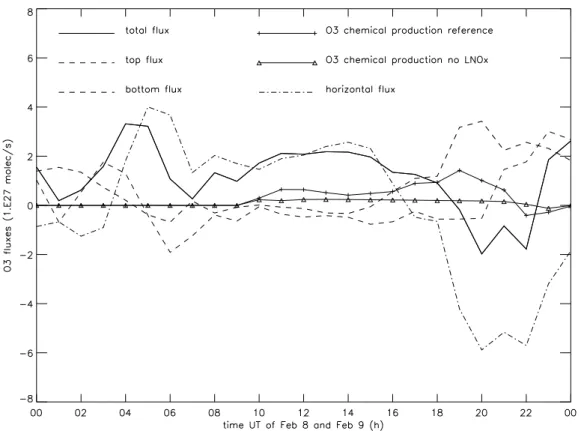
The O₃fluxes are calculated every hour for each side of the domain as follows:

15 F_s = 10−6 100. k_{bol tz} ZZ S P_{ai r}(i , j, k) T_{ai r}(i , j, k) n(i , j, k).V (i , j, k) O3(i , j, k) d S (1) where F_s (in molec/s) is the flux through the surface S of the domain, k_{bol tz} is the Boltzmann constant, P_{ai r} and T_{ai r} are, respectively, the pressure (in hPa) and the tem-perature (in K), O₃is the ozone concentration (in molec cm−3), i , j and k are the usual indices for directions x, y, and z. n is the unit vector perpendicular to the elementary

20

surface d S, and V is the velocity vector. The sign of the flux is chosen to be positive when entering the TTL domain and negative when exiting it. Results of this calculation are shown in Fig. 8 and the 24 h integrated results are reported in Table 1. A 24 h period has been chosen in order to encompass a full ozone production/destruction di-urnal cycle. The total flux reported in Fig. 8 is the sum of the fluxes for each side of

(16)

ACPD

5, 9169–9205, 2005

– Part II

Print Version

the domain plus the chemical ozone production inside the domain for the “reference” run. The corresponding ozone production for the “no LNO_x” run is also reported as an indication.

5.1. Total flux and horizontal flux

The total flux, is always positive, except between 19:00 UT and 22:00 UT. This

ex-5

plains why the O₃concentration generally increases during this period, except between 16:00 UT and 20:00 UT as it was previously seen in Fig. 1 (see Sect. 2.3).

The horizontal flux is characterised by two different dynamical regimes. The first regime, until 16:00 UT, depicts most of the time positive values of the flux. It is char-acterised by a maximum at 05:00 UT of 4×1027molec/s (which is the maximum of all

10

the fluxes considered), followed by an almost constant value of 2×1027molec/s un-til 15:00 UT. The second regime is characterized by a decrease of the flux, leading to negative minimum value of −6×1027molec/s at 20:00 UT (which is also the abso-lute minimum of all the fluxes considered). The horizontal flux increases again after 22:00 UT but is still negative. This change of dynamical regime, correlated to the high

15

convective activity, is explained by the change of direction of the wind in the western part of grid 2: during the first period the winds were mostly along the western edge of Grid 2 (northward direction), while during the second period, the winds on this side of the domain turn to the north-west direction, increasing the ozone flow out of the grid. It is noted that the total flux follows roughly the time evolution of the horizontal flux,

20

due to its relatively large values and variability compared to the other fluxes. However, when integrated on a 24 period (see Table 1), the contribution of the horizontal flux is relatively weak (−9% of the total ozone increase) due to the fact that the large minimum of the second regime compensates the positive values of the first regime.

(17)

ACPD

5, 9169–9205, 2005

– Part II

Print Version

5.2. Chemical production inside the TTL

The contribution of the chemical ozone production inside the TTL for both simulations is also shown in Fig. 8. For the “reference” run, the maximum of this contribution (∼1.5×1027molec/s) is relatively weak compared to the other contributions, but when integrated over 24 h, it represents 23.5% of the total ozone increase. The ozone

chem-5

ical production is zero during night-time, increases after sunrise and remains constant until 16:00 UT. From this time which corresponds to the beginning of the intense period of convection, the ozone increases again, due to the fact that ozone precursors are lifted up to the TTL by deep convection and that LNO_xis produced. During the most in-tense period of convection (around 22:00 UT), it is worth noting that the contribution of

10

the ozone production is negative. This is because this period also coincides with sun-set, and the ozone amount around 14 km at this time is comparable with the amount of NO_x. Thus, ozone is destroyed by NO_x at sunset, because of O₃ titration. The maxi-mum of convection, if shifted in time with respect to sunset, would have increased the contribution of chemical production in the TTL ozone budget.

15

For the “no LNOx” simulation, the behaviour is qualitatively comparable with the re-sults of the “reference” run, but the production of ozone is quantitatively much less. For the 24 h integration period, the O₃ production inside the TTL without LNO_x represents 36% of the ozone production with LNO_x. This result stresses the local role of LNO_x in producing ozone directly inside the TTL, even if the maximum of ozone LNO_x

produc-20

tion is below the TTL, as shown in Fig. 5. The role of LNO_x in producing ozone inside the TTL is emphasized during the intense period of convection.

In Fig. 5, it should be noted the ozone production at 13 km is 3 times stronger for the “reference” run than for the “no LNO_x” run. This induces a level of ozone at 13 km which is higher for the reference run than for the no “LNO_x run”. This might have an

25

impact in the calculation of the vertical flux at 13 km which is proportional to the O₃ concentration at 13 km multiplied by the vertical velocity.

(18)

ACPD

5, 9169–9205, 2005

– Part II

Print Version

5.3. Vertical flux at the bottom of the TTL

The vertical flux at 13 km is expected to give an important indication of how O₃ chem-ically produced below the TTL (see Figs. 5 and 6) can be transported into the TTL. This flux oscillates around a zero value until 16:00 UT. From this time its contribution is always positive and becomes the largest contribution in the ozone budget. This is

5

once again correlated with the convective activity in the simulation which is very intense during this period.

As deduced from Table 1, the overall contribution of the flux at the bottom of the TTL is 75% of the total ozone increase for this 24 h period. This high ratio is logical considering that this flux is almost all the time positive during the 24 h period, while the

10

other fluxes have a succession of negative and positive values, which weakens their contribution in the total ozone increase.

In order to estimate the contribution of the chemistry in this upward O₃flux, we have compared the bottom flux for the “reference” run and the “no LNO_x” run for the same 24 h period in Fig. 9. The calculation of the same flux for the “no LNO_x” simulation

15

provides values that are similar to those of the “reference” run. Differences only ap-pear from 09:00 UT. From this time and until 16:00 UT, the “no LNO_x” 13 km flux is slightly higher than for the “reference” run. This result is logical considering that the O₃ amounts are higher for the “reference” run than for the “no LNO_x” run and that the vertical motions are downward on average during that period.

20

From 16:00 UT the “reference run” flux calculations are higher than the “no LNO_x” calculations. The differences between the simulations are higher during that period than for the 09:00 UT to 16:00 UT period. Considering that the upward motions prevail from 16:00 UT, corresponding to an intense period of convection, this result illustrates the role of convection in bringing O₃produced by LNO_x up to the TTL, or locally

pro-25

ducing ozone by LNO_x at 13 km.

By integrating the differences of both fluxes on this 24 h period, it can be shown that the 13 km flux for the “reference” run is only 3% higher than for the “no LNO_x” run. This

(19)

ACPD

5, 9169–9205, 2005

– Part II

Print Version

value is small considering the difference of ozone production between the “reference” and the “no LNOx” simulations. Most of the differences between the simulations for the 13 km flux occur around the convective cells (not shown). A detailed analysis of the dynamics (which is the same for both simulations) and the ozone production chemistry around convective cells shows that ozone which is produced by LNO_x can be

trans-5

ported up to the TTL. In the “no LNO_x” run, ozone is transported up to the bottom of the TTL but the amount of ozone in the outflow of the cell is lower since the chemical production inside the convective tower is lower. In addition, at a convective scale, there is a local production of ozone by LNO_xat 13 km as shown in Fig. 5.

The consequence at the grid 2 scale is that the amount of ozone at 13 km is lower

10

for the “no LNO_x” run than for the “reference” run. However, for mass conservation rea-sons, convection generates downdrafts to balance updrafts. These downdrafts appear in the vicinity of the convective cells in our simulation. Since the amount of ozone at 13 km is higher for the “reference” run than for the “no LNO_x” run, the ozone upward fluxes are higher and the downward fluxes are lower (higher in absolute value) for the

15

“reference” run than for the “no LNO_x” run. The result for the 13 km flux for the domain defined in Fig. 7 is the sum of the contributions of the upward and downward fluxes, so that the difference between the simulations is relatively small.

The contribution of the flux at the bottom of the TTL could possibly be more impor-tant if the simulation was continued for a longer period since this could allow ozone

20

chemically produced by LNO_x at 12 km to be more transported into the TTL, or the LNO_xproduced at 12 km to be transported during the night to 13 km, where O₃can be produced chemically after sunrise. From Sects. 5.2 and 5.3 it can be concluded that, from the point of view of the ozone increase in the TTL, lightning produced NO_xplay a more important role in producing locally ozone than in producing ozone below the TTL

25

(20)

ACPD

5, 9169–9205, 2005

– Part II

Print Version

5.4. Vertical flux close to the tropopause

As mentioned earlier in this section, the top flux does not illustrate directly the role of STE in this TTL ozone budget. It can however give an indication of what is hap-pening in the tropopause region. This contribution is negative between 05:00 UT and 20:00 UT, but its 24 h integrated value is positive, corresponding to 11% of the total

5

ozone increase. This value is relatively small compared to the 13 km flux in Table 1, but not negligible and this contribution is high between 21:00 (8 February) and 00:00 UT (9 February) with values higher than 2×1027molec/s, comparable with the 13 km flux values. It is worth noting that the sharp increase of this contribution is correlated with an increase of the wave activity in the tropopause region, as illustrated in Fig. 10. This

10

figure provides the vertical velocity at 17 km (thus close to the tropopause level) for 12:00 UT and 23:00 UT. For both times, a wave activity exists in the simulation, as shown by an alternation of upward and downward motions inside Grid 2, centred on places where the convection is the most intense. It also shows that the vertical motions are much stronger for 23:00 UT than for 12:00 UT. This is related to deep convection

ac-15

tivity which generated gravity waves at the tropopause. Convection generated-waves are known to be isentropic. This means that the waves oscillate on iso-θ surfaces. However if these waves break, the motion is not isentropic anymore and can cross iso-θ surface. These breaking waves potentially bring stratospheric ozone down to the upper troposphere. We then talk of stratosphere to troposphere transport (or STT), according

20

to the nomenclature of Stohl et al. (2003). Two cases are possible for our simulation. Either the waves oscillate on iso-θ surfaces and on average, should not contribute to the ozone budget (the amount that crosses down the 17 km surface would cross up the same surface a half period of the wave later, so that the average budget is zero), or the waves break, an thus the average vertical transport is not zero, leading to STE. A full

25

study with higher vertical resolution would be necessary to quantitatively estimate the STE and to conclude about the interpretation of the 17 km flux given here. However, in the present simulations there are several convective cells developing close in time

(21)

ACPD

5, 9169–9205, 2005

– Part II

Print Version

and space. Thus there are several sources of waves. This is illustrated in the bottom panel of Figure 10 where two waves develop around two convective cells located at 49.8◦E 22◦S, and 47.5◦E 20.6◦S which can interact and provoke perturbations. These perturbations favour wave breaking (Albert Hertzog, personnal communication). Fur-thermore the increase of the top flux between 19:00 UT and 23:00 UT is relatively long

5

compared to the quarter of the period of the wave. This period is generally of a few hours. If this hypothesis is confirmed, our result would be compatible with the con-clusions of Wang et al. (1995). Performing a 2-dimensional model simulation of the ozone redistribution by a convective storm in the Pacific Ocean, they have shown that the stratospheric ozone had a significant contribution in the composition of the upper

10

troposphere. Olsen et al. (2002) using total column ozone observations and potential vorticity field analysis, reached the same conclusion.

5.5. Budget summary

As a consequence of the time evolution of each contribution in the TTL ozone budget, the ozone evolution in the TTL can be explained by the sum of each contribution.

15

Between 8 February at 00:00 UT and 09:00 UT, the ozone amount in the TTL increases, mainly due to the horizontal flux. After that, until 14:00 UT, the increase is due both to the horizontal flux and the chemical ozone production. Before the horizontal flux becomes negative, the ozone increase is due to both the chemical production and the vertical bottom flux, as a consequence of the strong convective activity. Between

20

17:00 UT and 22:00 UT when the total flux is negative, the high contribution of the bottom and tropopause fluxes partially compensate the large minimum of the horizontal flux. From 22:00 on 8 February to 00:00 on 9 February, the ozone increase is due the vertical fluxes at the bottom and the top of the TTL.

To summarise, this section shows that the behaviour of ozone in the TTL during the

25

period of convection is mainly due to the dynamics, the chemistry being responsible for ∼23.5%. This contribution could have been higher for cases with intense convection out of the sunset period. The vertical dynamics, especially at the end of the period of

(22)

ACPD

5, 9169–9205, 2005

– Part II

Print Version

calculation, is strongly related to deep convection: atmospheric waves generated at the top of the convection might favour the penetration of higher amounts of stratospheric ozone down to the TTL, and vertical flux at the bottom of the TTL plays the major role in the budget since it represents 75% of the total ozone increase on the 24 h period of the budget calculation, since this contribution is almost always positive. The correlation

5

between the chemical ozone production inside the TTL and the convection activity is also highlighted in this budget.

6. Conclusion and perspectives

In this study we have performed a simulation of a severe convective event which oc-curred on 8 February 2001 in Brazil, with a mesoscale model with on-line chemistry,

10

in order to investigate the ozone behaviour in the upper troposphere. The companion paper (Part I: Mar ´ecal et al., 2005) focussed on the meteorological simulation and on the ozone precursor results. They showed the average importance of deep convection in the vertical transport of ozone precursors from the surface to between 10 and 15 km altitude. They also showed the importance of lightning produced NO_xin the chemistry

15

of other ozone precursors in the upper troposphere, between 8 and 15 km.

We can summarise the main results of the second part of this series of papers as follows. During the severe convective event, the disturbed layer of ozone in the TTL simulated by the model qualitatively and quantitatively reproduces the set of DMI O₃ sonde observations from Bauru during the 2004 wet season. On average, an inflection

20

around 15 km in the ozone vertical profile is reproduced. Qualitatively, the variability of the ozone in the fine grid of the simulation is comparable with the ozone sonde obser-vations: a high variability in the TTL and a much lower variability above the tropopause. A budget of ozone in the TTL was calculated during 24 hours including the convective event. Firstly, it should be stressed that during the most intense period of the

con-25

vection, a strong signature of the convective activity was detected in the vertical flux at 13 km, in the downward motions around the tropopause and in the ozone chemical

(23)

ACPD

5, 9169–9205, 2005

– Part II

Print Version

production inside the TTL. Secondly, this 24 h budget shows that this increase of ozone in the TTL with respect to the initial state is mainly due to the dynamics, but with a sig-nificant contribution of the chemistry. In this case study, the major contribution in the budget is the vertical flux at the bottom of the TTL which accounts for 75% of the total O₃increase because this contribution is almost always positive during the 24 h period.

5

This contribution increases with the convection activity. It has been shown that 3% of this contribution is due to the lightning produced NO_x chemistry. A part of this 75% is due to chemical production of ozone below the TTL which is transported higher in the TTL by deep convection. The chemical production of ozone within the TTL is smaller but is significant since it represents 23.5% of the ozone budget. Finally we have found

10

that stratosphere to troposphere transport associated with convection-generated grav-ity wave breaking can occur. A complete high resolution study is needed to exactly quantify this contribution. In the present case, chemical production plays a weaker role than the dynamics in the TTL O₃ distribution. One of the explanations is that the maximum of the chemical production occurs at 12 km, on average, and is thus below

15

the bottom of the TTL. A significantly longer simulation might change this ratio since it could allow the ozone chemically produced around 12 km to be transported into the TTL by the large scale ascent. It could also allow the LNO_x produced during the night below the TTL to be transported up to 13 km, where O₃can be produced after sunrise. It could also allow the LNO_x produced above 13 km to form ozone after sunrise.

How-20

ever, a longer simulation would lead to a different type of study, since it would imply a larger domain of simulation. In our simulation results, the chemical production is mainly due to the presence of LNO_x in the upper troposphere even though it was shown that ozone precursors other than LNO_x also contributed to this chemical production. Com-parison of simulation results with or without the parameterisation of LNO_x shows that

25

the ozone production is enhanced by a factor of 4 when the lightning parameterisation is switched on.

This study shows that a mesoscale model with on-line chemistry is a powerful tool to study the chemistry in relation with deep convection: it can explicitly resolve the

(24)

ACPD

5, 9169–9205, 2005

– Part II

Print Version

convection, and can take into account a relatively large area around the event studied. Direct measurements to compare with model outputs are needed to better estimate the quality of the modelling results. This will be done in the future by studying events from the HIBISCUS/Troccinox/Troccibras 2004 field campaign, from which we can ob-tain information on H₂O, O₃, CO, NO_x, and halogen VSLS. The chemistry of halogen

5

species will be then included in the model, as well as the explicit O_xchemistry to better constrain the chemistry in the stratosphere. Another study of a convective system in the same area will determine if the O₃behaviour computed here can be reproduced. Acknowledgements. This modelling study is supported by funds from the 5th PCRD

(HIBIS-CUS project) and the French Centre National de le Recherche Scientifique (Programme

Na-10

tional de Chimie Atmosph érique). This work makes use of the RAMS model, which was devel-oped under the support of the National Science Foundation (NSF) and the Army Research Office (ARO). Computer resources were provided by CINES (Centre Informatique National de l’Enseignement Sup érieur), project pce2227. The authors thank V.-H. Peuch from M ét éo France for providing the MOCAGE fields that were used to initialise the chemistry model.

15

G. Foret from LaMP is also thanked for helping with the use of the chemistry model. We are grateful to A. Hertzog at Laboratoire de M ´et ´eorologie Dynamique, Palaiseau, for his comments about gravity waves generated by convection.

References

Aumont, B., Jaecker-Voirol, A., Martin B., and Toupance, G.: Tests of some reduction

hypothe-20

ses made in photochemical mechanisms, Atmos. Environ., 30, 2061–2077, 1996.

Brewer, A. M.: Evidence for a world circulation provided by measurements and vater vapour distributions in the stratosphere, Q. J. R. Meteorol. Soc., 75, 351–363, 1949.

Cotton, W. R., Pielke Sr., R. A., Walko, R. L., Liston, G. E., Tremback, C. J., Jiang, H., McAnelly, R. L., Harrington, J.-Y., Nicholls, M. E., Carrio, G. G., and McFadden, J. P.: RAMS 2001:

25

Current status and future directions, Meteorol. Atmos. Phys., 82, 5–29, doi:10.1007/s00703-001-0584-9, 2003.

Dessler, A. E.: The effect of deep, tropical convection on the tropical tropopause layer, J. Geophys. Res., 107(D3), 4033, doi:10.1029/2001JD000511, 2002.

(25)

ACPD

5, 9169–9205, 2005

– Part II

Print Version

Dickerson, R. R., Huffman, G. J., Luke, W. T., Nunnermacker, L. J., Pickering, K. E., Leslie, A. C. D., Lindsey, C. G., Slinn, W. G. N., Kelly, T. J., Daum, P. H., Delany, A. C., Greenberg, J. P., Zimmerman, P. R., Boatman, J. F., Ray, J. D., and Stedman, D. H.: Thunderstorms: an important mechanism in the transport of air pollutants, Science, 235, 460–465, 1987. Folkins, I., Braun, C., Thompson, A. M., and Witte, J.: Tropical ozone as an indicator of deep

5

convection, J. Geophys. Res., 107(D13), doi:10.1029/2001JD001178, 2002.

Holton, J. R., Haynes, P. H., McIntyre, M. E., Douglass, A. R., Rood, R. B., and Pfister, L.: Stratosphere-Troposphere exchange, Rev. Geophys., 33, 403–439, 1995.

Jourdain, L.: Mod élisation des oxydes d’azote et de l’ozone dans le mod èle de circulation g én érale LMDzT-INCA: r ôle des émissions par les éclairs et par l’aviation subsonique, PhD

10

Thesis, Universit ´e Paris 6, July 4th, 2003.

Komhyr, W. D., Barnes, R. A., Brothers, G. B., Lathrop, J. A., and Opperman, D. P.: Elec-trochemical concentration cell ozonesonde performance evaluation during STOIC 1989, J. Geophys. Res., 100, 9131–9244, 1995.

Labrador, L. J., von Kuhlmann, R., and Lawrence, M. G.: Strong sensitivity of the global mean

15

OH concentration and the tropospheric oxidizing efficiency to the source of NOx from

light-ning, Geophys. Res. Lett., 31, L06102, doi:10.1029/2003GL019229, 2004.

Mar ´ecal, V., Rivi `ere, E. D., Held, G., Cautenet, S., and Freitas, S.: Modelling study of the impact of deep convection on the UTLS air composition – Part I: analysis of the ozone precursors, Atmos. Chem. Phys. Discuss., 5, 9127–9168, 2005,

20

SRef-ID: 1680-7375/acpd/2005-5-9127.

Olsen, M. A., Douglass, A. R., and Schoeberl, M. R.: Estimating the downward cross-tropopause ozone flux using column ozone and potential vorticity, J. Geophys. Res., 107, 4636, doi:10.1029/2001JD002041, 2002.

Peuch, V.-H., Amodei, M., Barthet, T., Cathala, M.-L., Josse, B., Michou, M., and Simon, P.:

25

MOCAGE, MOd èle de Chimie Atmosph érique à Grande Echelle, Proceedings of M ét éo-France workshop on atmospheric modelling, December 1999, 33–36, 1999.

Pickering, K. E., Wang, Y., Tao, W.-K., Price, C., and M ¨uller, J.-F.: Vertical distributions of lightning NO_x for use in regional and global chemical transport models, J. Geophys. Res., 103(D23), 31 203–31 216, 1998.

30

Pielke, R. A., Cotton, W. R., Walko, R. L., Tremback, C. J., Lyons, W. A., Grasso, L. D., Nicholls, M. E., Moran, M. D., Wesley, D. A., Lee, T. J., and Copeland, J. H.: A comprehensive mete-orological modeling system – RAMS, Meteorol. Atmos., 49, 69–91, 1992.

(26)

ACPD

5, 9169–9205, 2005

– Part II

Print Version

Pundt, I., Pommereau, J.-P., Chipperfield, M. P., Van Roozendael, M., and Goutail, F.: Climatol-ogy of the stratospheric BrO vertical distribution by balloon-borne UV-Visible spectrometry, J. Geophys. Res., 107(D24), 4806, doi:10.1029/2002JD002230, 2002.

Ray, E. A., Moore, F. L., Elkins, J. W., Dutton, G. S., Fahey, D. W., V ¨omel, H., Oltmans, S. J., Rosenlof, K. H.: Transport into the Northern Hemisphere lowermost stratosphere

5

revealed by in situ tracer measurements, J. Geophys. Res., 104(D21), 26 565–26 580, doi:10.1029/1999JD900323, 1999.

Schoeberl, M. R.: Extratopical stratosphere-troposphere mass exchange, J. Geophys. Res., 109(D13), 303, doi:10.1029/2004JD004525, 2004.

Stohl, A., Bonasoni, P., Cristofanelli, P., et al.: Stratosphetroposphere exchange: A

re-10

view, and what we have learned from STACCATO, J. Geophys. Res., 108(D12), 8516, doi:10.1029/2002JD002490, 2003.

Taghavi, M., Cautenet, S., and Foret, G.: Simulation of ozone production in a complex circula-tion region using nested grids, Atmos. Chem. Phys., 4, 825–838, 2004,

SRef-ID: 1680-7324/acp/2004-4-825.

15

Taupin, F. G., Bessafi, M., Baldy, S., and Bremaud, P. J.: Tropospheric ozone above the south-western Indian Ocean is strongly linked to dynamical conditions prevailing in the tropics, J. Geophys. Res., 104(D7), 8057–8066, doi:10.1029/98JD02456, 1999.

Thompson, A. M., Witte, J. C., Oltmans, S. J., et al.: Southern Hemisphere Additional Ozonesondes (SHADOZ) 1998–2000 tropical ozone climatology 2. Tropospheric

variabil-20

ity and the zonal wave-one, J. Geophys. Res., 108(D2), 8241, doi:10.1029/2002JD002241, 2003.

Thorntorn, D. C., Bandy, A. R., Blomquist, B. W., Bradshaw J. D., and Blake, D. R.: Verical transport of sulfur dioxide and dimethyl sulfide in deep convection and its role in new particle formation, J. Geophys. Res., 102, 28 501–28 509, 1997.

25

V ¨omel, H., Oltmans, S. J., Johnson, B. J., Hasebe, F., Shiotani, M., Fujiwara, M,. Nishi, N., Agama, M., Cornejo, J., Paredes, F., and Enriquez, H.: Balloon-borne observations of water vapor and ozone in the tropical upper troposphere and lower stratosphere, J. Geophys. Res., 107(D14), doi:10.1029/2001JD000707, 2002.

Wang, C., Crutzen, P. J., Ramanathan, V., and Williams, S. F.: The role of a deep convective

30

storm over tropical Pacific Ocean in the redistribution of atmospheric chemical species, J. Geophys. Res., 100(D6), 11 509–11 516, 1995.

(27)

ACPD

5, 9169–9205, 2005

– Part II

Print Version

J. Geophys. Res., 105, 22 269–22 297, 2000.

WMO (World Meteorological Organization), Scientific Assessment of Ozone Depletion: 2002, Global Ozone Research and Monitoring Project – Report, No. 47, Chapter 2: Very short-lived halogen and sulphur substances, 2.1–2.57, Geneva, 2003.

(28)

ACPD

5, 9169–9205, 2005

– Part II

Print Version

Table 1. Integrated number of molecules of ozone entering the domain drawn in Fig. 7 during

a 24 h period starting from 02/08/2001 00:00 UT (in 1030molec) for the “reference” run. The horizontal, the top, bottom and the chemical contributions are reported. A positive value means a gain for the domain. Also shown are the percentage contributions to the ozone molecule increase.

total Top (17 km) Bottom (13 km) Horizontal Chemistry

1.E30O₃molec 103. 11.4 77.2 −9.7 24.2

(29)

ACPD

5, 9169–9205, 2005

– Part II

Print Version

Fig. 1. Temporal evolution of the O₃mean profile in the vertical range [8 km; 26 km] computed at regular 4 h time intervals by RAMS in Grid 2 between 8 February 2001 at 00:00 UT and 9 February 2001 at 04:00 UT. The initial state is also shown (black line). The horizontal scale is logarithmic.

(30)

ACPD

5, 9169–9205, 2005

– Part II

Print Version

Fig. 2. Same as in Fig. 1 but for O₃standard deviation normalised by the mean vertical profiles in Fig. 1.

(31)

ACPD

5, 9169–9205, 2005

– Part II

Print Version

Fig. 3. DMI sonde O₃measurements from Bauru, Brazil, during HIBISCUS 2004, expressed in the same vertical resolution as the RAMS model. The date of each launch is given in the figure. Also shown is the mean profile of all the measurements (black thick solid line), the mean vertical profiles of ozone computed by RAMS in Grid 2 at 12:00 UT on 7 February 2001 (initial state), and at 00:00 UT on 9 February 2001 for the “reference” run. The horizontal scale is logarithmic.

(32)

ACPD

5, 9169–9205, 2005

– Part II

Print Version

(33)

ACPD

5, 9169–9205, 2005

– Part II

Print Version

Fig. 5. Vertical profile of the mean accumulated chemical ozone production in Grid 2 of the

RAMS model until 8 February 00:00 UT, 8 February 12:00 UT, 9 February 00:00 UT.(a)

(34)

ACPD

5, 9169–9205, 2005

– Part II

Print Version

Fig. 6. Mean of the ozone variation in the altitude range [8 km; 18 km] computed by RAMS in

Grid 2 8 February 00:00 UT, 8 February 12:00 UT, 9 February, 00:00 UT. The results including LNO_xare presented using thick lines, and the results without LNO_x are shown using thin lines.