Monte Carlo entropic sampling applied to Ising-like model for 2D and 3D systems

HAL Id: insu-01313920

https://hal-insu.archives-ouvertes.fr/insu-01313920

HAL is a multi-disciplinary open access archive for the deposit and dissemination of sci-entific research documents, whether they are pub-lished or not. The documents may come from teaching and research institutions in France or abroad, or from public or private research centers.

L’archive ouverte pluridisciplinaire HAL, est destinée au dépôt et à la diffusion de documents scientifiques de niveau recherche, publiés ou non, émanant des établissements d’enseignement et de recherche français ou étrangers, des laboratoires publics ou privés.

Monte Carlo entropic sampling applied to Ising-like

model for 2D and 3D systems

Catalin-Maricel Jureschi, Jorge Linares, Pierre-Richard Dahoo, Yasser Alayli

To cite this version:

Catalin-Maricel Jureschi, Jorge Linares, Pierre-Richard Dahoo, Yasser Alayli. Monte Carlo entropic sampling applied to Ising-like model for 2D and 3D systems. Journal of Physics: Conference Series, IOP Publishing, 2016, 738, pp.012051. �10.1088/1742-6596/738/1/012051�. �insu-01313920�

Open Access Journal of Physics: Conference Series (JPCS) (in press)

Monte Carlo entropic sampling applied to Ising-like model for

2D and 3D systems

C M Jureschi1,2_{, J Linares}3,*_{, P R Dahoo}4_{, Y Alayli}1

1 _{LISV, UVSQ, Université Paris Saclay, 78140 Vélizy, France.}

2 _{Faculty of Electrical Engineering and Computer Science & MANSiD, USV,} Suceava, 720229, Romania.

3 _{GEMaC, UVSQ, Université Paris Saclay, 78035 Versailles Cedex, France.} 4 _{LATMOS, UVSQ, Université Paris Saclay, F-78280, Guyancourt.}

E-mail: jorge.linares@uvsq.fr

Abstract. In this paper we present the Monte Carlo entropic sampling (MCES) applied to an

Ising-like model for 2D and 3D system in order to show the interaction influence of the edge molecules of the system with their local environment. We show that, as for the 1D and the 2D spin crossover (SCO) systems, the origin of multi steps transition in 3D SCO is the effect of the edge interaction molecules with its local environment together with short and long range interactions. Another important result worth noting is the co-existence of step transitions with hysteresis and without hysteresis. By increasing the value of the edge interaction, L, the transition is shifted to the lower temperatures: it means that the role of edge interaction is equivalent to an applied negative pressure because the edge interaction favours the HS state while the applied pressure favours the LS state. We also analyse, in this contribution, the role of the short- and long-range interaction, J respectively G, with respect to the environment interaction, L.

1. Introduction

Simulation of physical processes is a challenge for scientists trying to understand how the physical processes that occur inside materials drive their properties. Thus, in physics besides analytical methods which can solve exactly either finite or infinite systems, there are also other numerical methods which can solve exactly or with an approximation only finite system. Monte Carlo methods are the most utilized ones by researches in order to model probabilistic or stochastic systems whose analytical solutions are too complicated or impossible to be obtained. Concerning SCO materials [1-3], the Monte Carlo methods are used in combination with certain models such as: Ising-like model, atom-phonon coupling (APC) model or mechanical-elastic model. All these models are used to simulate the evolution of SCO materials when they are subjected to external perturbations such as: thermal or/and pressure variation, light irradiation, applied external magnetic or electrical fields. The importance granted to these materials is due to their potential application in displays, nanoelectronics, data storage or as temperature or/and pressure sensors. These materials which are characterized by two stable states, a diamagnetic low spin (LS) state and a paramagnetic high spin (HS) state, present the great advantage that they can be controlled at the atomic level.

Open Access Journal of Physics: Conference Series (JPCS) (in press)

Recent investigations using Monte Carlo methods applied to an Ising-like model [4-6] have shown that the behaviour of SCO materials is influenced by the network architecture of the system, the system’s size or the size of particles [7]. Also, the role of edge effects for 1D, 2D and 3D SCO network systems has been reported by considering that the edge molecules are fixed in HS states. Some important results have been reported in the recent years for 1D and 2D SCO network system when the edge molecule are active.

In this work the role of edge molecules as active molecules that interact with their local environment are analyzed using MCES method applied to an Ising-like model.

2. The model

To represent the two spin states of molecules, Wajnflasz et al. [4] introduced a spin operator, σ, which can take the value -1 when the molecule is in the LS state and the value +1 when the molecule is in the HS state. The degeneracy ratio of the two spin states is given by g g _HS /g_LS. In this context, by taking into account the interaction of edge molecules with their local environment and by considering the edge molecules as active molecules, Chiruta et al. [8] added a new parameter, L, to the Ising type Hamiltonian. For a system of N molecules with Ns edge molecules the Hamiltonian is given by:

1 , 1 1 ln 2 t t s N N N B i i j i i i i j i i k T g H 









where Δ is the gap energy, kB is Boltzmann constant, J is the short range interaction and G is the long range interaction.

Defining the dimensionless macroscopic variable, m, s and c as:

1 , ' 1 , s N i i j i i j N k k m  s   and c       







the Hamiltonian from equation (1) can be written as: ln 2 B k T g H_    G  _m Js Lc    , (3) where ln 2 B f k T g h  _    G  _  . (4)

According to the Hamiltonian from equation (3), the average magnetization can be written as follows:

1, 1, 1 ( )exp ( ) 1 ( )exp ( ) i i i i f i i i i NL B i i i f i i i i NL B m d m s c h m Js Lc NL k T d m s c h m Js Lc k T                         





where NL is the number of distinct configuration of states <m,s,c> and d(m,s,c) is the number of configuration for a given set of values.

3. Monte Carlo Entropic Sampling

We used the Monte Carlo entropic sampling (MCES) method described by Shteto et al. [9,10] to generate a table that contains the dimensionless macroscopic variables, m, s, c , and their density, d(m,s,c) that is the degeneracy of the macrostate (m,s,c). The principle of MCES is that to obtain a

Open Access Journal of Physics: Conference Series (JPCS) (in press)

desired distribution P, it is necessary to introduce an appropriate distribution as a bias in the detailed balance equation expressed as:

  

( ) ( )

i j

PW i j P W j i , ₍₆₎

and the biasing probability was chosen as the inverse of the desired restricted density of states. 1 ( , , ) i i i i P d m s c  , ₍₇₎

In this way, configurations with weakly degenerate macrostates are favored and those with highly degenerate states are damped. In this case, the detailed balance equation (6) can be written as:

( , , ) ( ) (j ) ( , , ) j i i i i j j j P d m s c W i j W i P d m s c  _{ }  . (8)

Because in the first Monte Carlo step the density of the state d(m,s,c) is unknown we put all d(m,s,c) equal to 1. So, after iteration k the density will be dk(m,s,c). Then, using dk(m,s,c) as a bias, a MC

sampling is ran; it is termed a ‘Monte Carlo stage’ and it yields a histogram of the frequency of the macrostates: Hk(m,s,c):







_{  }

The resulting restricted density of states is obtained after applying a correction for the bias:













1 , ,  , , , ,

k k k

d m s c d m s c H m s c . (10

From the table of the d(m,s,c) thus built from the (m, s, c) states, the partition function can be calculated using the following expression:

 



from which all the thermodynamic properties of the system can be analytically derived.

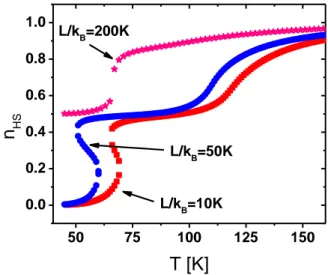
50 75 100 125 150 0.0 0.2 0.4 0.6 0.8 1.0 L/k_B=200K L/k B=50K

n

T [K]

Figure 1. The thermal behaviour for a 3D SCO system for different values of parameter L. The computational parameters are: Δ/kB = 600 K, J/kB = -40 K, G/kB = 200 K, ln(g) = 6, N = 125 (5 x 5 x 5).

Open Access Journal of Physics: Conference Series (JPCS) (in press)

In figure 1 is presented the influence of edge effects. As we can see, by increasing the parameter value of the edge molecules interaction with their local environment, the transition is shifted to the low temperature and if it is strong enough then the transition is incomplete and without hysteresis.

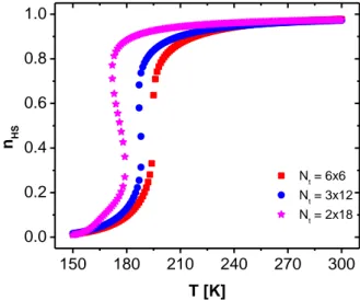
The role of the system’s shape was analyzed in the last years [11]. It is well known that thermal behaviors of systems with the same number of molecules but with different shapes differs from one system to another. As was reported by Chiruta et al [11], a chain system consisting of 1600 molecules shows less cooperativity than in a ladder system or a square system containing the same number of molecules. So, the transition for a chain system is more gradual, even without hysteresis, compared to a ladder or a square system where the transition is abrupt and with a large hysteresis width. In figure 2 is reported the thermal behaviors for a system with different shapes but with edge effect. As we can see in figure 2 the behavior is strong influenced by the edge effect. By decreasing the system’s cooperativity the transition is shifted to lower temperatures and occurs with hysteresis.

150 180 210 240 270 300 0.0 0.2 0.4 0.6 0.8 1.0 N_t = 6x6 Nt = 3x12 Nt = 2x18 nHS T [K]

Figure 2. The thermal behaviour for different shapes of a 2D system containing 36 molecules. The computational parameters are: Δ/kB = 1300 K, J/kB = 15 K, G/kB = 172.7 K, L/kB = 120K, ln(g) = 6.01, N = 36. 4. Conclusions

In this work we studied the thermal behaviour for an Ising-like system under submitted to edge effects. In this context we used MCES method applied to an Ising-like model (where the edge effect is represented by the L parameter) to show the influence of edge effect in 2D and 3D SCO systems. It is important to mention that the edge interaction favors the HS state and that by increasing the value of parameter L or by increasing the ratio between the number of edge and inner molecules, the transition is shifted to the lower temperature.

Acknowledgments

CHAIR Materials Simulation and Engineering, UVSQ, Université Paris Saclay is gratefully acknowledged.

References

[1] Gütlich P 2013 European Journal of Inorganic Chemistry 2013 581-91

[2] Harding D J, Harding P and Phonsri W 2016 Coordination Chemistry Reviews 313 38-61 [3] Jureschi C M, Linares J, Boulmaali A, Dahoo P, Rotaru A and Garcia Y 2016 Sensors 16 187 [4] Wajnflasz J and Pick R 1971 J. Phys. Colloques 32 C1-91-C1-2

[5] Bousseksou A, Nasser J, Linares J, Boukheddaden K and Varret F 1992 Journal De Physique I 2 1381-403

Open Access Journal of Physics: Conference Series (JPCS) (in press)

[6] Boukheddaden K, Linares J, Codjovi E, Varret F, Niel V and Real J A 2003 Journal of Applied Physics 93 7103-7105

[7] Muraoka A, Boukheddaden K, Linares J and Varret F 2011 Physical Review B 84 http://dx.doi.org/10.1103/PhysRevB.84.054119

[8] Chiruta D, Jureschi C-M, Linares J, Dahoo P, Garcia Y and Rotaru A 2015 The European Physical Journal B 88 1-5

[9] Shteto I, Linares J and Varret F 1997 Physical Review E 56 5128-37

[10] Linares J, Enachescu C, Boukheddaden K and Varret F 2003 Polyhedron 22 2453-2456

[11] Chiruta D, Jureschi C-M, Linares J, Garcia Y and Rotaru A 2014 Journal of Applied Physics 115 - doi: 10.1063/1.4864035