Structure of the low-latitude magnetopause: MAGION-4 observations

HAL Id: hal-00316240

https://hal.archives-ouvertes.fr/hal-00316240

Submitted on 1 Jan 1997

HAL is a multi-disciplinary open access archive for the deposit and dissemination of sci-entific research documents, whether they are pub-lished or not. The documents may come from teaching and research institutions in France or abroad, or from public or private research centers.

L’archive ouverte pluridisciplinaire HAL, est destinée au dépôt et à la diffusion de documents scientifiques de niveau recherche, publiés ou non, émanant des établissements d’enseignement et de recherche français ou étrangers, des laboratoires publics ou privés.

Structure of the low-latitude magnetopause:

MAGION-4 observations

Z. Nemecek, A. Fedorov, J. Safrankova, G. Zastenker

To cite this version:

Z. Nemecek, A. Fedorov, J. Safrankova, G. Zastenker. Structure of the low-latitude magnetopause: MAGION-4 observations. Annales Geophysicae, European Geosciences Union, 1997, 15 (5), pp.553-561. �hal-00316240�

Structure of the low-latitude magnetopause: MAGION-4 observations

1

Faculty of Mathematics and Physics of Charles University, Prague, Czech Republic

2_{Space Research Institute, Academy of Sciences of Russia, Moscow, Russia}

Received: 12 December 1995 / Revised: 14 October 1996 Accepted: 16 October 1996

Abstract. The aims of this paper are (1) briefly to

describe the plasma devices onboard the MAGION-4 satellite, launched on 3 August 1995, of the INTER-BALL project, and (2) to discuss first observations made near the magnetopause region. During the presented boundary crossings the MAGION-4 observed quasi-periodic pulses of magnetosheath-like plasma in a region of low plasma density. This region is located just earthwards of the magnetopause and is populated by a plasma which, except for the density, has the same parameters as in the magnetosheath. Deeper in the magnetosphere, the encounter of a layer of hot electrons and high-energy ions was interpreted as low-latitude boundary layer.

1 Introduction

The Earth’s magnetopause lies at the locus of points where magnetosheath and magnetospheric pressures balance. Since the magnetosheath pressure at the subsolar point is proportional to the solar-wind dynamic pressure (Landau and Lifshitz, 1959), observations of the solar-wind dynamic pressure can be used to predict magnetopause motion. A number of recent studies (Sibeck et al., 1989 a,b; Potemra et al., 1989) have demonstrated that brief, sharp increases in the solar-wind dynamic pressure, each lasting from 1–10 min, are common just upstream of the bow shock. Such pulses are often quasi-periodic with recurrence time-scales of 5–15 min. Their origin remains unknown, although sources in the solar wind and at the quasi-parallel bow shock have been suggested (Sibeck et al., 1989 a,b). They must be considered as a major source of transient magnetopause motion.

The observations made by ISEE 1/2 at the northern-dawn magnetopause were interpreted as evidence of the diffusive entry of magnetosheath plasma into the mag-netosphere and of Kelvin-Helmholtz instability at the inner edge of the Low-latitude boundary layer (LLBL)

(Sckopke et al., 1981). They have also been interpreted by different authors as indicating magnetic merging and the formation of twisted ropes of interconnected mag-netosheath and magnetospheric magnetic lines (Pas-chmann et al., 1982; Cowley, 1982, 1984, 1986; Saunders, 1983). The flux tube or rope develops both for stationary and non-stationary conditions in the diffusion region (the region where the magnetic field is not frozen into the plasma). Except for singular cases, these flux tubes move along the magnetopause and therefore represent transient events for any fixed loca-tion. The formation of such magnetic flux tubes requires the onset of magnetic reconnection or a strong intensi-fication of the reconnection rate.

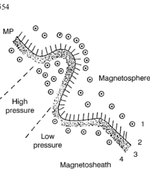
An alternative mechanism for transient magnetic perturbations is a wavy motion of the magnetopause boundary layer driven by fluctuations of the solar-wind dynamic pressure (Sibeck, 1992, 1993). Sibeck et al. (1990) showed that FTEs [flux transfer events (Russell and Elphic, 1978)] are fully consistent with the proper-ties of magnetosheath magnetic field line draping in the plasma depletion layer, and they presented a model for the signatures of magnetopause motion driven by such solar-wind dynamic-pressure variations. Figure 1 shows a cross-section of the magnetopause in the plane parallel to the ecliptic plane and indicates the expected magne-topause response to a brief increase in the solar-wind dynamic pressure. Such an increase corresponds to an enhancement in both magnetosheath thermal and mag-netic pressures which in turn compress the magneto-pause locally to form a trough. As the trough approaches a spacecraft in the magnetosphere, that spacecraft observes an increase in the magnetic-field strength. If the spacecraft, exits the magnetosphere and enters the magnetosheath, it should observe streaming energetic ions, a colder, denser, antisunward flowing plasma, and a magnetosheath magnetic-field orientation in the plasma depletion layer.

The scheme of the magnetopause structure depicted in Fig. 1 is widely accepted, but the criteria for the identification of the magnetopause layers can vary in

different papers. Russell (1995) shows that for north-ward-oriented magnetic field the plasma depletion layer (sheath transition layer) is separated from the magne-tosheath by a current layer which causes the magnetic-field rotation towards the magnetospheric orientation. The plasma depletion layer itself is characterized by the gradual decrease in the plasma density. This layer is bounded by the other current layer on its inner edge from the LLBL. The LLBL is populated by plasma with the temperature and density intermediate between those of the magnetosheath and the magnetosphere, and the magnetic field has magnetospheric orientation. The boundary between the LLBL and magnetosphere has no signature in the magnetic field and can be identified by the fast increase in the plasma temperature.

During the periods of the southward magnetic field the first turn in the magnetic field which divides the magnetosheath and magnetopause layers is not followed by the decrease in the plasma density. The LLBL is characterized by the high temperature and magneto-spheric magnetic field. Phan and Paschmann (1996) introduces the magnetic shear (the angle between magnetic-field vectors inside and just outside the mag-netopause) for the classification of the magnetopause crossings. This classification respects the fact that the IMF can change its direction in front of the magneto-pause due to the turbulent motion of the magnetosheath plasma. In general, the low-shear magnetopause struc-ture corresponds to that observed during the southward period of the IMF, and the high-shear magnetopause is similar to that observed if the IMF is southward. Phan and Paschmann (1996) define the magnetopause as the beginning of the magnetic-field rotation and the inner edge of the LLBL as the point where the plasma density decreases to 5% of the magnetosheath value.

The present paper introduces the measurements in the magnetopause region performed by a set of plasma instruments onboard the MAGION-4 INTERBALL subsatellite. The set consists of two experiments: the VDP-S plasma sensor is dedicated to the fast

determi-nation of the ion- and electron-flux vector. The MPS/ SPS part measures the electron- and ion-energy distri-bution function in several directions. Based on the data collected so far and supplemented by the magnetic-field measurement we try to identify the structure of the dawn low-latitude magnetopause layers and to estimate the origin of different plasma populations found in these layers.

2 Instrumentation

This section describes the plasma devices placed on-board the MAGION-4 satellite in detail; such a description cannot be found elsewhere, the information given in Triska et al. (1995) being very brief. The INTERBALL project is predominantly dedicated to the study of the Earth’s magnetotail, but the satellite spent a long time in the solar wind and the magnetosheath. Thus the plasma devices should cover a wide range of measured quantities.

The main portion of the solar-wind energy is repre-sented by the ion bulk velocity, and thus precise and fast measurement of the ion-flow parameters is required. On the other hand, inside magnetospheric boundaries and in the magnetotail, the hydrodynamic approximation cannot be used, and detailed knowledge of the ion- and electron-energy distribution is of ultimate importance. The VDP-S – MPS/SPS complex is supposed to fulfil all the requirements mentioned; the designs are based on experiments previously flown onboard Prognoz-type satellites: the MONITOR experiment onboard the Prognoz-8 (Zastenker et al., 1982; Avanov et al., 1985) and the BM device which was part of the BIFRAM spectrometer onboard the Prognoz-10 satellite (Bed-rikov et al., 1985). The main idea is that for different scientific tasks, different types of sensors are used. This approach simplifies each sensor design and increases the instrument reliability. It should be stressed that due to the reduced available mass and power allocations onboard the MAGION-4 subsatellite, experiments have been made as simple as possible to fulfil their scientific objectives. In accordance with this idea the instruments onboard the MAGION-4 satellite are composed of three parts:

– A set of four Faraday’s cups (FCs) for the determi-nation of the total ion-flow vector (e.g. Avanov et al., 1984).

– Two cylindrical electrostatic analysers for a precise determination of the ion velocity and temperature looking in the sunward and antisunward directions. The cylindrical analysers have a narrow entrance angle (~ 3°) and provide a one-dimensional cut of the ion-velocity distribution. Santolik et al. (1991) showed that this does not influence the computed values of the velocity and temperature under a wide range of measurement conditions.

– Two hemispheric electrostatic analysers for the deter-mination of the ion- and electron-energy distribution in several directions.

Fig. 1. The wavy downside magnetopause boundary. The

magneto-sphere is labelled 1, the low-latitude boundary layer as 2, the plasma depletion layer as 3, and the magnetosheath as 4 (from Sibeck et al.

1990)

This set of detectors can provide all basic hydrody-namic parameters which can be compared with more complex measurements taken onboard the main, IN-TERBALL-1 satellite. The simplification of the MAG-ION-4 devices in comparison with their analogues onboard the main satellite follows from stringent requirements on the weight and power consumption.

2.1 Plasma-flow detector VDP-S

For the determination of the integral flux and of the direction of the bulk velocity of incoming particles the VDP-S device is based on the simultaneous measure-ments of the currents of four identical FCs which are placed symmetrically on the subsatellite’s surface with axes declined from the main subsatellite’s axis by ~ 45°. Due to the satellite in-flight orientation, the axis of the first FC is directed nearly towards the Sun. Due to the negative voltage ()170 V) which is supplied permanently to the suppressor grid, the VDP-S device registers the sum of all ions and electrons with an energy greater than 170 eV. The negative voltage value exceeds considerably the possible energy of the secondary electrons and photoelectrons arising under the action of the Sun’s UV radiation and thus eliminates the contribution of these electrons to the total collector current. The other grids of the FC system are connected to the body of the subsatellite. The size of the collector, diameters of apertures and the distances between the grids are chosen so that the angular characteristics of the sensor have a triangular shape with a width of ˆ50° on zero level. These characteristics are a result of the compromise between the optimal ±90°view angles and the sensor size. The principal electrical schematic of the VDP-S detector is given in Fig. 2. The collector of the FC is

connected to the electrometric amplifier which is placed just under a particular FC to minimize the input capacitance. The amplifier output is connected to a low-pass filter. The bandwidth of the filter can be controlled from the Earth in agreement with the telemetry bit rate to keep the signal cut-off frequency in accordance with the Nyquist criterion. Filter outputs are multiplexed to the input of a logarithmic AD converter (ADC). The logarithmic conversion gives us the possibility to compress the polarity and the signal value with the dynamics of four orders of magnitude to eight bits with relative accuracy: ± 3%. The frequency of the multiplexing is changed from the Earth according to the telemetry bit rate and to the number of bytes designed for the VDP-S device in the particular tele-metry structure. To increase the sampling frequency by decreasing a spatial coverage, a mode in which only signals from two FCs are transmitted can be switched on via a command.

2.2 MPS/SPS plasma spectrometers

The MPS spectrometer was dedicated predominantly to the continuous monitoring of solar-wind parameters and for the registration of reflected ions from the bow shock. In the Earth’s tail region the orientation of the MPS device along the Sun-Earth line was expected to allow the estimation of the ion leakage from the ionosphere as well as the search for counter-streaming ion beams. Due to the inclination of the actual rotational axis from the expected one, these advantages of the MPS have been lost and the MPS data can serve as a supplement to the data of the SPS spectrometer, a device which was designed for the rough determination of the angular distribution of ions and electrons and for fast measurement of their energy distribution. The angular field of view of the MPS and SPS detectors is depicted schematically in Fig. 3. One can note that the declination of the rotational axis did not change the sense of the SPS data substantially but that some part of the velocity space remained without coverage.

The MPS and SPS energy spectrometers are quite similar and most of the electronic circuits are common to both of them.

The MPS system consists of two identical sensors which are placed along the main subsatellite’s axis in opposite directions. The ions come through the entrance collimator, the cylindrical electrostatic analyser and are multiplied by a channeltron. Before multiplication the ions are accelerated by the channeltron supply voltage to obtain sufficient efficiency at low energies. The schematic plot of one MPS section is given in Fig. 4.

The SPS spectrometer contains two hemispheric analysers, one for electrons, the other for ions. The particles are registered by microchannel plates (MCP) with divided collectors. This set-up has a relatively high geometric factor and allows a rough estimation of the pitch-angle distribution. From the plot in Fig. 5, where the electron section of the SPS device is shown, it can be seen that the electrons are accelerated by ~150 V, which

is formed by the Zenner diode from the MCP supply voltage. The electrons from the MCP output are accelerated to the collector which is split into two parts. Each of these two collectors is connected to its own

amplifier and Schmitt trigger. The ion section of the SPS device is nearly identical, the difference is in the MCP supply circuits and in the number of collectors only. Ions are accelerated by the full MCP supply voltage and the ion collector is divided into three parts.

The supply voltages for channeltrons and MCPs are trimmed individually and can be changed in four steps by an Earth’s command independently for each detec-tor. The analyser voltage is common to both spectro-meters (SPS and MPS) and can be swept in a range of 4÷ 2500 V. This range is divided into two subranges: 4÷ 500 V for solar-wind measurements and 20÷2500 V predominantly designed for magnetospheric measure-ments. The subrange as well as the number of steps (4, 8 or 16) inside the subrange can be chosen by command. The ratio between the analyser voltage and the corre-sponding energy is ≈ 10 for both spectrometers. The actual values of all high voltages are monitored by one multiplexed analogue telemetry channel.

Pulses from channeltrons or MCP collectors are amplified, shaped and counted by 18-bit counters. Four times per telemetry frame the counting is stopped and the logarithm of the contents of the counters is taken to obtain 8-bit output words. The results are sent to the telemetry together with the information on the current energy step.

3 Data processing

The actual rotational axis of the MAGION-4 satellite is declined from the expected one by about ~ 40°, and this value changes from orbit to orbit. This situation changes significantly the orientation of the detectors relative to the Sun-Earth line and brings many complications in the determination of plasma parameters such as, e.g., the velocity vector. For this reason the data are presented in the satellite’s frame. The data have been received during real-time transmission sessions. Due to poor quality of the transmission we had to remove all blocks with a bad check sum and this procedure caused gaps in the data. Further careful processing will allow to fill in many of these gaps.

4 Preliminary experimental results

Figure 6 presents the ion- and electron-energy spectro-grams which have been obtained by the SPS system of the MAGION-4 satellite during 29 August 1995, from 085500 to 091500 UT. At the beginning of this time-interval the MAGION-4 satellite was located at GSE

(X,Y,Z) ˆ (10, )71, )11) × 103km and moved nearly along the Y-axis towards the Earth with a velocity of 2.6 km s)1. The subsatellite was followed by the INTER-BALL-1 satellite separated by 1020 km.

Three different regions denoted by A, B and C can be identified in the spectrograms. The A region, until 085720 UT, is characterized by an intensive, nearly isotropic electron distribution (no modulation by the subsatellite’s rotation can be seen). This type of distri-bution was observed for more than 2 h preceding the time-interval depicted in Fig. 6. On the other hand,

Fig. 3. Schematic plot of the MPS and SPS detectors’ orientation

Fig. 4. Schematic plot of the MPS sensor (one section)

Fig. 5. Schematic plot of the electron part of the SPS sensor

measurements of the ion distribution are affected by the satellite’s spin. It indicates that the bulk velocity of the ion flow exceeds the thermal one. The shape of the electron and ion distributions in this region can be seen in Fig. 7a. The electrons show a typical flat-top distribution, the ion distribution exhibits a broad maximum which corresponds to a bulk velocity of about ~ 230 km s)1. The ion temperature estimated from this distribution is about ~ 7×105K. The shape of these energy distributions together with the spacecraft position indicate that this region is the magnetosheath. The B region starts at 085720 UT when the energy and intensity of registered electrons decreases and the ion flow nearly vanishes. The energy spectra in Fig. 7b which have been taken in this region indicate that despite the density of ions and electrons being low, the origin of the plasma is the same as in the A region. Intermittent low-density and magnetosheath plasma regions are detected till 091040 UT. Energy spectra in Fig. 7c have been measured inside one of the magneto-sheath intervals at 090529 UT.

The C region begins at 091040 UT, when a significant increase in the electron energy is associated with the decrease in the intensity of registered ions (Fig. 7d). There can be two reasons for this decrease: (1) a real decrease in the ion density, or (2) an increase in the ion energy out of our measuring range.

The three plasma regions mentioned can be clearly distinguished in the FC data as depicted in Fig. 8. The currents are in units of the voltage on the amplifier output. This voltage is roughly proportional to the ion density through the regions A and B because the

electron current is negligible in these regions and the plasma-velocity variation is of the order of 10%. The FC0 (top panel) is oriented along the actual space-craft rotation axis, and thus its data are not affected by the rotation. Inside the A region this FC measures the ion current higher than the upper limit of the amplifier (10)10A). The actual value of the input current can be estimated from FC 1 as 1.7×10)10A. It corresponds to a density of about ~ 10 cm)3. The B region starts at 085720 UT by a sharp decrease in the ion current to nearly zero. This low background level is characteristic for the whole region, but above this background five sharp positive current spikes are detected. The B region ends at 091030 UT when all the FCs register nearly isotropic electron current.

5 Discussion

The principal question in the interpretation of the data is when the magnetopause was crossed. For the crossing, we have two possible candidates: the extinc-tion of the ion current at 085720 UT and the electron boundary at 091030 UT. The parameters of the ion flow at the beginning of the considered interval in the A region are clearly those of the magnetosheath; high-energy electrons (in the C region) can be attributed either to the LLBL or to the inner magnetosphere. Unfortunately, we cannot complete our observation by the reliable magnetic field measurements taken on the MAGION-4 satellite because its SGR magnetometer was designed for comparative measurements only.

Fig. 6. Ion-and electron-energy dynamic spectrograms of the magnetopause crossing observed on 29 August by the MAGION–4 satellite. From all channels of the SPS device only those with

maximum count rate are shown. Grey scales are in counts, the counting time was 150 ms for each energy step

Moreover, the unexpected orientation of the satellite axis still did not allow to recalculate the data to the physical coordinate system. On the other hand, we can compare our data with the measurements of the INTERBALL-1, satellite which was only 1000 km away (Safrankova et al., 1996).

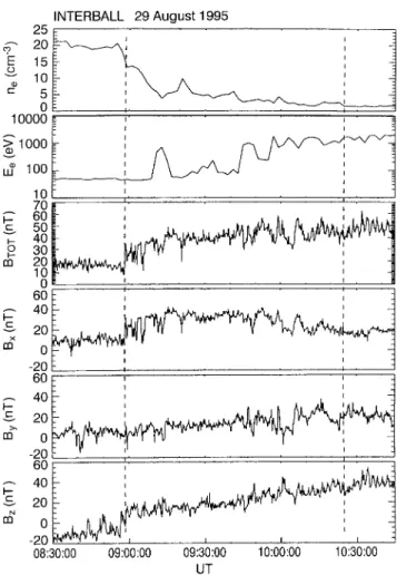
Figure 9 shows the macroscopic structure of the event. The rotation of the magnetic field together with the increase in its value occurs at ~ 0900 UT, the electron density completes its falling at ~ 1025 UT. At the same time the electron temperature reaches its magnetospheric value. In accordance with Phan and Paschmann (1996), we can attribute the first boundary to the magnetopause and the second one to the inner edge of the LLBL. The considerable time-lag between these two boundaries is connected with the fact that the solar-wind pressure and the IMF were exceptionally stable during this time-interval and there was no reason for macroscopic magnetopause motion. If only the satellite velocity is taken into account, the thickness of the whole magnetopause-LLBL system is 1.6 RE.

It is necessary to note that according to the model of Sibeck et al. (1991) the expected distance of the magnetopause from the Earth under actual conditions in the solar wind measured by the WIND spacecraft (pressure 2.5 Pa, IMF BZ~ )2.5 nT between 0600 and

0900 UT) was 16.8 RE, but the boundary was crossed at

the distance of 14.1 RE. Careful examination of the data

showed that there is no indication of any crossing of any boundary between 0645 and 0850 UT.

The magnetopause crossing on a smaller scale, as measured by the INTERBALL-1 satellite, is illustrated in Fig. 10. The Figure shows the same time-interval as Figs. 6 and 8, because for this time-interval the data from both satellites are available. The magnetic field is given in the boundary normal coordinates where BNis

taken as the minimum variance direction of the magnetic field for the period depicted in Fig. 6, BL is

the maximum variance direction in the plane perpen-dicular to N and BMcompletes the right-hand set.

The first rotation of the magnetic field occurs at 085630 UT, when the ion density starts to fall. This

Fig. 7 a-d. Ion- and electron-energy spectra in different plasma regions (a magnetosheath, b low-density region, c magnetosheath-like region, d LLBL). The corresponding plasma parameters computed from the

spectra are: a -v1= 214 km s)1, Ti= 90 eV, Te= 28 eV, b vi= 198 km

s)1, Ti= 110 eV, Te= 23 eV, c vi= 214 km s)1, Ti= 110 eV, Te= 27

eV, d vi, Ti– not determined, Te= 221 eV

boundary can be interpreted as the outer boundary of the plasma depletion layer. At the second distinct boundary (at 085840 UT) the magnetic field changes its value from 13 to 33 nT, but the direction remains unchanged except for short bipolar excursions of the BN

and BMcomponents, which indicate the presence of thin

current layers on the boundary. The decrease in the ion density by a factor of 5 coincides with the increase in the magnetic field. We can suggest that this boundary is the magnetopause itself.

Afterwards the magnetic field and the plasma density change their values a few times nearly to the magneto-sheath ones till 091015 UT. This time corresponds to the beginning of the C region in Figs. 6 and 8 when the current of the FCs becomes negative (the flux of electrons with energy greater than 170 V becomes higher than the ion current) and thus it cannot be used for a reliable determination of the ion density. The electron density in Fig. 9 continues its decrease through the boundary and the electron temperature increases. This boundary has no signature in the magnetic field and according to Russell (1995) it can be classified as the transition to the inner part of the LLBL.

The ion-density enhancements observed afterwards can be interpreted as consecutive intensive encounters with the magnetopause because the value and fluctua-tions of the magnetic field are similar to those in the

magnetosheath. Similar observations of multiple ion-density enhancements made by the ISEE 2 have been interpreted as the crossing of the ion edge of the LLBL (Gosling et al., 1990). The authors suggested that the intermittent appearance of the density enhancements is caused either by the varying position of the boundary or by a non-stationary reconnection process. In our case, however, the character of the plasma inside the small regions with enhanced ion density corresponds clearly to the magnetosheath because no evidence of ion acceler-ation is found (Nemecek et al., 1997).

The regions of low ion and electron density around ion-density enhancements cannot be considered as be-longing to the plasma depletion layer because this layer should be located outside the magnetopause. We suppose that regions are part of the LLBL, which is characterized by the permanently open field lines, and the particles which penetrate through the magnetopause are blown down. However, the origin and mechanism of the creation of the observed layer, which is characterized by ~ 1/10 of the magnetosheath plasma density and magne-tospheric magnetic-field intensity, and which is located just earthward of the magnetopause, remain unclear.

The quasi-periodic appearance of the magneto-sheath-like plasma here is probably caused either by a wavy magnetopause motion, similar to that depicted in

Fig. 8. Faraday’s cup currents during the same event as in Fig. 6 Fig. 9. Overall view of the magnetopause crossing as measured by INTERBALL-1 satellite. The dashed lines denote the magnetopause (left) and the inner edge of the LLBL (right)

Fig. 1, or by flux ropes which connect the reconnection site at the magnetopause with the magnetosphere. Sibeck et al. (1990) noted that the signatures of these two cases are similar and a clear distinction can be made only after further data processing. Since the density enhancements are inside the depleted region, which probably lies on the permanently open field lines, a wavy motion of the boundary seems to be preferable for the interpretation.

The inner layer populated by hot electrons has been identified as the LLBL because the broad energy spectra are similar to those observed in the cleft region. In this case we can suppose that the energy of ions exceeds our measuring range, which is consistent with the observa-tions presented in Fig. 6.

6 Conclusion

The paper presents the first results of the plasma measurements in the magnetopause region carried out by the MAGION-4 satellite. Preliminary processing of the data leads to the conclusion that the boundary layer located earthwards of the magnetopause consists of two regions: a low-density layer of the magnetopause, and the low-latitude boundary layer.

Despite the IMF being oriented southward, the crossing under study has all features reported by Russell (1995) for the cases with the northward IMF. We suggest that the classification of the crossings according the IMF-BZ direction can be used only for the dayside

magnetopause where the magnetic field inside the LLBL has northward orientation. The local time in our case was about six o’clock and the magnetic field inbound of the magnetopause was oriented nearly along the XGSE

axis. For such a case, the classification according to the magnetic shear is more appropriate.

Further processing of the MAGION-4 data together with the data from the INTERBALL-1 satellite can probably provide the means for a better understanding of this event, as these satellites were separated only by about ~ 1000 km in the direction nearly perpendicular to the magnetopause surface during this particular mag-netopause crossing.

Acknowledgements. The help of a number of colleagues who

contributed to the VDP-S and MPS/SPS proposals and to the preparation of the devices is gratefully acknowledged. The last stages of the experiment preparation have been supported by the Czech Grant Agency under Contracts 205/96/1575 and 202/94/ 0467. The development and construction of the MAGION-4 satellite and its scientific payload have been supported by the Czech Grant Agency under Contract 102/93/0882. Authors express their thanks to M. Ciobanu for supplying the SGR magnetic field data. Topical Editor K.-H. Glaßmeier thanks J. Bu¨chner and J. Sauvaud for their help in evaluating this paper.

References

Avanov, L. A., G. N. Zastenker, O. L. Vaisberg, Yw. I. Yermolaev, Observation of small-scale solar-wind structure during the sharp increase of plasma flow velocity (in Russian) Kosmich.

lssl., 22, 774, 1984.

Avanov, L. A., A. Leibov, Z. Nemecek, J. Safrankova, O. Vaisberg, J. Yermolaev, G. Zastenker, Fast measurements of solar-wind parameters by the MONITOR instrument, in: INTERSHOCK

project, Ed. S. Fischer, Public. of AI CAS, 60, 39, 1985.

Bedrikov, A., A. Belikova, A. Fedorov, V. Fuchs, V. Hanzal, V. Kuzmin, A. Leibov, S. Namestnik, Z. Nemecek, V. Notkin, M. Richter, J. Safrankova, O. Vaisberg, J. Yermolaev, G. Zastenker, Complex of plasma spectrometers BIFRAM, in:

INTERSHOCK project, Ed. by S. Fischer, Public. of AI CAS,

60, 113, 1985.

Cowley, S. W. H., The causes of convection in the Earth’s magnetosphere: A review of developments during the IMF, Rev.

Geophys., 20, 531, 1982.

Cowley, S. W. H., Solar-wind control of magnetospheric convec-tion. Achievements of the International Magnetospheric Study IMS, ESA SP-217, ESTEC, Noordwijk, Netherlands, 483, 1984 Cowley, S. W. H., The impact of recent observations on theoretical understanding of solar wind-magnetosphere interaction. J.

Geomagn. Geoelectr., 38, 1223, 1986.

Gosling, J. T., M. F. Thomsen, S. J. Bame, and T. G. Onsager, The electron edge of the low-latitude boundary layer during acce-lerated flow events, Geophys. Res. Lett., 17, 1833, 1990. Landau, L. D., and E. M. Lifshitz, Fluid Mechanics, Pergamon,

New York, 1959.

Nemecek, Z., J. Safrankova, O. Santolik, K. Kudela, E. T. Sarris, Energetic particles in the vicinity of the dawn magnetopause,

Adv. Space Res., in print, 1997.

Paschmann, G., G. Haerendel, I. Papamastorakis, N. Sckopke, S. J. Bame, J. T. Gosling, and C. T. Russell, Plasma and magnetic Fig. 10. Comparison of the plasma parameters and magnetic field

measured by the INTERBALL 1 and MAGION-4 satellites

field characteristics of magnetic flux transfer events, J. Geophys.

Res., 87, 2159, 1982.

Phan, T. D., and G. Paschmann, Low-latitude dayside magneto-pause and boundary layer for high magnetic shear, 1. Structure and motion, J. Geophys, Res., 101, 7801, 1996.

Potemra, T. A., H. Luehr, L. J. Zanetti, K. Takahashi, R. E. Erlandson, G. T. Marklund, L. P. Block, L. G. Blomberg, and R. P. Lepping, Multisatellite and ground-based observations of transient ULF waves, J. Geophys. Res., 94, 2543, 1989. Russell, C. T., The structure of the magnetopause, in Physics of the

Magnetopause, ed. P. Song et al. Geophysical Monograph, 90,

81–98, 1995.

Russell, C. T., and R. C. Elphic, Initial ISEE magnetometer results: Magnetopause observation, Space Sci. Rev., 22, 681, 1978. Safrankova, J., G. Zastenker, Z. Nemecek, A. Fedorov, M.

Simersky, and L. Prech, Small-scale observation of the magne-topause motion: Preliminary results of the INTERBALL project, this issue, 1996.

Santolik, O., J. Safrankova, and Z. Nemecek, The method of thermodynamics calculation and its application on the study of protons and alpha particles behaviour in the bow shock, Czech,

J. Phys., B 41, 381, 1991.

Saunders, M. A., Recent ISEE observations of the magnetopause and low-latitude boundary layer: A review, J. Geophys., 52, 190, 1983.

Sckopke, N., G. Paschmann, G. Haerendel, B. U. O. Sonnerup, S.J. Bame, T. G. Forbes, E. W. Hones Jr., and C. T. Russell, Structure of the low-latitude boundary layer, J. Geophys. Res., 86, 2099, 1981.

Sibeck, D. G., Transient events in the outer magnetosphere: Boundary waves or FTE’s?, J. Geophys. Res., 97, 4009, 1992. Sibeck, D.G., Transient magnetic field signatures at high latitudes,

J. Geophys. Res., 98, 243, 1993.

Sibeck, D. G., W. Baumjohann, R. C. Elphic, D. H. Fairfield, J. F. Fennell, W. B. Gail, L. J. Lanzerotti, R. E. Lopez, H. Luehr, A.T.Y. Lui, C. G. Maclennan, R. W. McEntire, T. A. Potemra, T. J. Rosenberg T. J., and K. Takahashi, The magnetospheric response to 8-min-period strong-amplitude upstream pressure variations, J. Geophys. Res., 94, 2505, 1989a.

Sibeck, D. G., W. Baumjohann W., and R. E. Lopez, Solar-wind dynamic pressure variations and transient magnetospheric signatures, Geophys. Res. Lett., 16, 13, 1989b.

Sibeck, D. G., R. P. Lepping, and A. J. Lazarus, Magnetic field line draping in the plasma depletion layer, J. Geophys. Res., 95, 2433, 1990.

Sibeck, D. G., R. E. Lopez, E. C. Roelof, Solar-wind control of the magnetopause shape, location, and motion, J. Geophys. Res., 96, 5489, 1991.

Triska, P., J. Voita, and Yu. Agafonv, The INTERRALL sub-satellite S2-A and S2-T, in INTERBALL Mission and Payload,

Ed. Yu. Galperin et al., CNES-IKI-RSA, 100, 1995.

Zastenker, G. N., J. I. Yermolajev, S. Pinter, Z. Nemecek, J. Safrankova, A. B. Belikova, A. V. Leibov, V. Prochorenko, A. E. Stefanovic, A. G. Bedrikov, B. T. Karimov, Solar-wind obser-vation with high time resolution (in Russian) Kosmich. 20, 900, 1982.