HAL Id: hal-00298448
https://hal.archives-ouvertes.fr/hal-00298448
Submitted on 30 Aug 2005HAL is a multi-disciplinary open access archive for the deposit and dissemination of sci-entific research documents, whether they are pub-lished or not. The documents may come from teaching and research institutions in France or abroad, or from public or private research centers.
L’archive ouverte pluridisciplinaire HAL, est destinée au dépôt et à la diffusion de documents scientifiques de niveau recherche, publiés ou non, émanant des établissements d’enseignement et de recherche français ou étrangers, des laboratoires publics ou privés.
Remote detection of water property changes from a time
series of oceanographic data
A. Henry-Edwards, M. Tomczak
To cite this version:
A. Henry-Edwards, M. Tomczak. Remote detection of water property changes from a time series of oceanographic data. Ocean Science Discussions, European Geosciences Union, 2005, 2 (4), pp.399-415. �hal-00298448�
OSD
2, 399–415, 2005 Remote detection of property changes A. Henry-Edwards and M. Tomczak Title Page Abstract Introduction Conclusions References Tables Figures J I J I Back CloseFull Screen / Esc
Print Version Interactive Discussion
EGU
Ocean Science Discussions, 2, 399–415, 2005 www.ocean-science.net/osd/2/399/
SRef-ID: 1812-0822/osd/2005-2-399 European Geosciences Union
Ocean Science Discussions
Papers published in Ocean Science Discussions are under open-access review for the journal Ocean Science
Remote detection of water property
changes from a time series of
oceanographic data
A. Henry-Edwards and M. Tomczak
School of Chemistry Physics and Earth Sciences, Flinders University of South Australia, GPO Box 2100, Adelaide SA 5001, Australia
Received: 27 June 2005 – Accepted: 16 August 2005 – Published: 30 August 2005 Correspondence to: M. Tomczak ([email protected])
OSD
2, 399–415, 2005 Remote detection of property changes A. Henry-Edwards and M. Tomczak Title Page Abstract Introduction Conclusions References Tables Figures J I J I Back CloseFull Screen / Esc
Print Version Interactive Discussion
EGU
Abstract
A water mass analysis method based on a constrained minimization technique is devel-oped to derive water property changes in water mass formation regions from oceano-graphic station data taken at significant distance from the formation regions. The method is tested with two synthetic data sets, designed to mirror conditions in the
5
North Atlantic at the Bermuda BATS time series station.
The method requires careful definition of constraints before it produces reliable re-sults. It is shown that an analysis of the error fields under different constraint assump-tions can identify which properties vary most over the period of the observaassump-tions. The method reproduces the synthetic data sets extremely well if all properties other than
10
those that are identified as undergoing significant variations are held constant during the minimization.
1. Introduction
In recent years, the general acceptance of global warming and the importance of long-range weather forecasting for modern agriculture have made climate change and
vari-15
ability an important issue. The interactions of the atmosphere and the ocean are of great importance for climate research, and many countries have made these processes a primary focus of their research programs. This has led to increased recognition of the role of the oceanic circulation for climate research and of water masses as elements of climate stability.
20
Within the broader category of climate research there are two major types of change to be investigated. Climate variability takes place over time scales of months, years or decades and is largely affected by year to year changes in oceanographic water mass formation. Climate change occurs over longer time periods of centuries or thousands of years. Prior to the 1980s, most climate research largely ignored both of these variations
25
OSD
2, 399–415, 2005 Remote detection of property changes A. Henry-Edwards and M. Tomczak Title Page Abstract Introduction Conclusions References Tables Figures J I J I Back CloseFull Screen / Esc
Print Version Interactive Discussion
EGU
atmosphere interact, with little consideration of temporal variability.
With increasingly powerful computers becoming available to oceanographers a large number of climate and ocean models have been developed, often on global scales. One of the key problems facing modellers is the accurate representation of water mass formation (England and Maier-Reimer, 2001). To this end, numerous tracers have been
5
incorporated into ocean models, either for data assimilation studies, model validation or as part of studies into the oceanic carbon cycle. Water masses integrate changes tak-ing place in the surface flux in ocean and climate models. This makes them attractive tools for the detection of climate change in a climate model (Banks et al., 2002).
Many water masses are formed in sub-polar regions, where continuous monitoring
10
of air and sea properties can be both expensive and hazardous. This is especially the case during the winter months when most of the water mass formation occurs. As a result of this, the properties of some water masses are only poorly understood. A greater understanding of the production of these water masses over long time periods and changes in their properties is therefore of great interest to climate researchers.
15
After the second world war a series of weather ships were deployed across the At-lantic and Pacific to provide time series of atmospheric measurements for weather fore-casts. Many of these ships also collected oceanographic data as standard procedure, leading to some extensive time series of temperature and salinity. With the deployment of weather satellites for the same purpose, many of the weather ships were phased out
20
and the oceanographic time series were stopped.
Increased interest in climate variability has seen a renewed interest in time series of oceanographic data. The Bermuda Atlantic Time-series Study (BATS) from the Sar-gasso Sea (Michaels and Knap, 1996; Steinberg et al., 2001) and the Hawaii Ocean Time-Series (HOTS) from Hawaii (Karl and Lukas, 1996) are two prominent
oceano-25
graphic time series, both of which have been running for quite some time collecting high quality monthly data. The ARGO floats being deployed around the world’s oceans also promise a large volume of ongoing oceanographic data. With the growing avail-ability of these and other time series, it is important to develop methods with which to
OSD
2, 399–415, 2005 Remote detection of property changes A. Henry-Edwards and M. Tomczak Title Page Abstract Introduction Conclusions References Tables Figures J I J I Back CloseFull Screen / Esc
Print Version Interactive Discussion
EGU
analyse and utilise the increasing volume of time dependent oceanographic data. Many existing water mass analysis techniques, in particular Optimum Multi-Parameter (OMP) analysis and isopycnal analysis, assume constant water mass prop-erties and are designed for looking at water mass contributions over a wide area with-out any temporal variation (Hinrichsen and Tomczak, 1993; Karstensen and Tomczak,
5
1998; Tomczak and Large, 1989). This approach is valid for analyses of individual cruises or data sets with no time dependence but is not always appropriate when look-ing at an oceanographic time series. Indeed, one of the primary principles of modern climate research is that oceanographic and atmospheric properties vary with time.
In a recent OMP analysis of the BATS data set in the Sargasso Sea near Bermuda
10
in the North Atlantic Leffanue and Tomczak (2004) found that the Labrador Sea Water (LSW) signal apparently disappeared from the data set for a number of years, at the same time as an increase in analysis error values was observed. They noticed that by introducing a time dependence of LSW salinity the error values were reduced and the LSW signal remained present throughout the entire time period. They concluded
15
that changes in the weather conditions over the Labrador Sea during water mass for-mation had resulted in variations in the properties of LSW which were then propagated throughout the North Atlantic, and which OMP analysis was unable to resolve.
With this in mind, this paper describes the development of a new water mass analysis tool which can be used to identify changes in source water properties as well as water
20
mass contributions from observations of temperature, salinity and other parameters such as oxygen and nutrients. We will be generating a simple simulated data set for this purpose, in which all source water properties as well as all relative contributions are prescribed and thus vary in a known manner. We then apply a technique based on OMP analysis to the data set to test the feasibility of the analysis. (We have chosen to
25
call the new technique Time Resolving OMP (TROMP) analysis to indicate its derivation from the original OMP analysis technique.) In a companion paper (Henry-Edwards and Tomczak, 2005) we apply the new method to the BATS data and show that it is capable of extracting information on variations of water mass properties in the Labrador Sea
OSD
2, 399–415, 2005 Remote detection of property changes A. Henry-Edwards and M. Tomczak Title Page Abstract Introduction Conclusions References Tables Figures J I J I Back CloseFull Screen / Esc
Print Version Interactive Discussion
EGU
from observations taken near Bermuda.
2. Data and method
Two simulated time series of station data were created to test the feasibility of a TROMP analysis. Both reflect conditions in the North Atlantic Ocean but with different degree of closeness to observations. In each data set the water properties Pi for all source
5
water masses were predefined through source water types SWTi, as were the relative contributions xi at which the water masses contribute to the simulated time series. These values were then combined using the linear mixing equation to produce the “measured” property values Pmeas=ΣxiPi to generate the time series.
The first simulated time series used source water properties for three water masses,
10
Western North Atlantic Central Water (WNACW), Labrador Sea Water (LSW) and Iceland-Scotland Overflow Water (ISOW). The source water type definitions were taken from Leffanue and Tomczak (2004), and WNACW was represented as a single source water type through values at the lower end of its distribution range. Time variations in the time series were produced by varying the salinity of Labrador Sea Water to match
15
that of Iceland-Scotland Overflow Water for a period and letting it return to its initial value thereafter. Table 1 gives the source water type definitions at the start of the time series; Fig. 1 shows the time development.
The second data set was based on more realistic variations of LSW temperature and salinity. It prescribed the same time-invariable oxygen and nutrient source water types,
20
included an upper definition for WNACW, and simulated time variations of tempera-ture as well as salinity, following the observations from the Labrador Sea described by Dickson et al. (1996).
Optimum Multi-Parameter (OMP) analysis was first introduced as an extension of the temperature-salinity mixing triangle (Tomczak, 1981). We refer the reader to available
25
descriptions for full details of the OMP analysis procedure (for example Karstensen and Tomczak, 1998) and restrict ourselves to a brief summary, as TROMP analysis is based
OSD
2, 399–415, 2005 Remote detection of property changes A. Henry-Edwards and M. Tomczak Title Page Abstract Introduction Conclusions References Tables Figures J I J I Back CloseFull Screen / Esc
Print Version Interactive Discussion
EGU
on OMP analysis. OMP analysis solves a system of linear mixing equations to identify the relative contributions of a number of source water types in a given data set. In an analysis of a data set in which four source water types are present and measurements for salinity (S), potential temperature (T ), oxygen (O), nitrate (N), phosphate (P) and silicate (Si) are used as tracers, the system of equations would take the form:
5 T1x1 + T2x2 + T3x3 + T4x4 = Tobs + RT S1x1 + S2x2 + S3x3 + S4x4 = Sobs + RS O1x1 + O2x2 + O3x3 + O4x4−α∆O = Oobs + RO N1x1 + N2x2 + N3x3 + N4x4+ α∆N = Nobs + RN P1x1 + P2x2 + P3x3 + P4x4+ α∆P = Pobs + RP
Si1x1+ Si2x2+ Si3x3+ Si4x4+ α∆Si = Siobs+ RSi x1 + x2 + x3 + x4 = 1 + RΣ
Here xi are the relative contributions from each source water type in the observed property distribution, α is a “pseudo age” of the water sample, ∆∗ are the Redfield ratios (Pahlow and Riebesell, 2000) and R are the residuals that are minimised to solve the equation. The last line of the equation is the mass constraint function to
10
ensure that the sum of water type contributions adds up to 100%. In the minimisation, a weighting function W is added and the equation is re-arranged to take the form:
R= W × (Ax − b) ,
where R is the residual, A is the matrix of source water types, x is the vector of rela-tive contributions and b is the vector of measured water properties. A non-negativity
15
constraint is introduced to avoid negative water mass contributions. By ensuring the number of water properties exceed the number of source water types in the analysis, the minimisation becomes an over-determined problem and is solved in a straightfor-ward manner.
Time Resolving Optimum Multi-Parameter (TROMP) analysis was designed to
iden-20
OSD
2, 399–415, 2005 Remote detection of property changes A. Henry-Edwards and M. Tomczak Title Page Abstract Introduction Conclusions References Tables Figures J I J I Back CloseFull Screen / Esc
Print Version Interactive Discussion
EGU
data. TROMP solves a similar system of equations to OMP. The main difference is that a TROMP analysis varies the source water properties as well as the relative contribu-tions.
The inclusion of source water properties as variables in the analysis means that the minimisation function becomes non-linear and highly under-determined. Such
sys-5
tems have an infinite set of solutions, and it is necessary to impose additional con-straints upon the minimisation in order to achieve a viable result. The main problem faced during the development of the TROMP method was the identification of suitable minimisation constraints and criteria to establish a procedure that leads to physically realistic and trustworthy results.
10
The TROMP analysis operates in two alternating stages; the first defines initial val-ues, while the second performs the actual minimisation. Stage 1 uses source water types to determine the relative contributions of each water mass through OMP analy-sis. Stage 2 takes the relative contributions determined from stage 1 and the source water type values from the previous time step as starting values for a constrained
min-15
imisation. Initialisation of the procedure, i.e. definition of source water types for the first time step, is either based on water type definitions from the literature or found through recourse to data from the water mass formation regions. The source water types for each following time step are defined as the results from the previous time step, meaning that the source water types can change smoothly with time.
20
A sequential quadratic programming method was used, which solves a quadratic programming sub-program at each iteration. The method is outlined in Gill et al. (1981) and Fletcher (1980) and implemented in the Matlab function fmincon.m, which was used for this project. Fixed variation limits are defined around each source water type and relative contribution.
25
In first attempts to use the TROMP analysis we allowed all source water properties to vary and placed only limits on their range of variation. This proved to be e ffec-tive for very simple data series with relaffec-tively large variations but was not suitable for data sets with more realistic source water variations. Experimentation with a range of
OSD
2, 399–415, 2005 Remote detection of property changes A. Henry-Edwards and M. Tomczak Title Page Abstract Introduction Conclusions References Tables Figures J I J I Back CloseFull Screen / Esc
Print Version Interactive Discussion
EGU
constraints and careful evaluation of the error fields led us to define an approach in which TROMP analysis only uses SWTs as variables that can reasonably be expected to have undergone significant variations, while keeping all other SWTs as constants. As we will show, information from the error fields can be used to identify which water type properties have to be set as variables, and which properties can be considered
5
constants.
3. Results and discussion
An essential aspect of any application of a constraint minimisation is the identification of suitable constraints. In an oceanographic context it is rarely obvious from the data which water type variations are the most important contributors to the observed
varia-10
tions of water properties. The first task of a TROMP analysis is therefore the relative ranking of possible variables in terms of their importance to the determination of a solution that comes as close as possible to reality.
An extensive series of trials produced pointers how to proceed. It easily confirmed our expectation that analyses that include all SWTs as variables do not produce
sen-15
sible results. Reducing the level of complexity only slightly, however, can provide leads on how to proceed: If one source water property is allowed to vary in all SWTs (while all other source water properties are kept constant), the analysis produced a distinct pattern in the error fields. This is clearly seen in the results from our first simulated data set, in which the only source water property that varied was salinity (and this variation
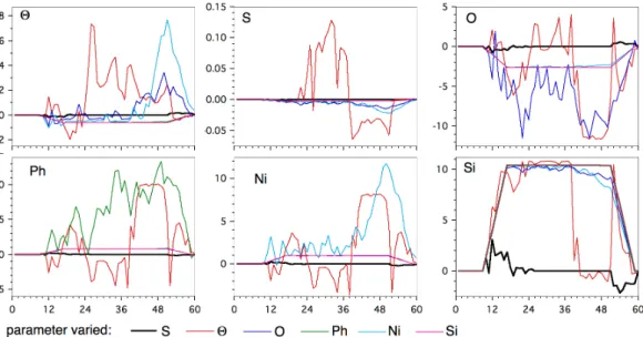
20
was restricted to LSW). Figure 2 shows the residual error for the six properties as func-tions of time. In most situafunc-tions the errors vary wildly and at times grow well beyond reasonable bounds, but they become quite small when salinity is allowed to vary in all SWTs (heavy curves in Fig. 2). Notice that this is true for all properties and not just for salinity, although only salinity was allowed to vary. This is a strong indication that the
25
most important change in the source water properties occurred in salinity.
OSD
2, 399–415, 2005 Remote detection of property changes A. Henry-Edwards and M. Tomczak Title Page Abstract Introduction Conclusions References Tables Figures J I J I Back CloseFull Screen / Esc
Print Version Interactive Discussion
EGU
in order of importance) it is then possible to proceed with a better targeted TROMP analysis by limiting the number of variables to one or two source water properties for a single SWT. The TROMP algorithm allows us to set limits on the variation of all variables, and the proposed procedure can be implemented by setting extremely narrow (or zero) variation limits for all SWT definitions except the one of interest (in our
5
case LSW salinity). The results of this approach were satisfactory for our first simulated data set, particularly when the analysis was implemented in two or more iterations of stages 1 and 2 for every time step. However, the analysis produced not only the correct time evolution of salinity but also apparent variations in potential temperature, a property that was set to remain constant in the simulated data set (Fig. 3).
10
The problem becomes more acute when the range of SWT variations is small, as in the actual time development of LSW properties, on which we based our second simulated data set. Figure 4 shows the results when TROMP analysis is applied to that data set in the manner just described. It is seen that the analysis traces the actual evolution of LSW potential temperature and salinity closely but contains much
15
unrealistic noise. TROMP analysis improves on the first guesses derived from OMP analysis; it reduces the departure from the correct relative contributions and the noise, but the reduction is rather small.
Applying a low-pass filter to the results can of course improve the agreement be-tween observations and analysis. A better way to improve the result can be obtained
20
by restricting the number of variables in the analysis: When all water type properties that are considered unimportant for the explanation of the observed property variations are not handled as variables with extremely narrow variation limits but are declared constants, the TROMP analysis is forced to concentrate on the variable of interest and produces excellent agreement between the simulated data and the results from the
25
OSD
2, 399–415, 2005 Remote detection of property changes A. Henry-Edwards and M. Tomczak Title Page Abstract Introduction Conclusions References Tables Figures J I J I Back CloseFull Screen / Esc
Print Version Interactive Discussion
EGU
4. Conclusions
A sequential quadratic programming method named TROMP analysis was applied to two synthetic data sets to simulate an analysis aimed at extracting variations of Labrador Sea Water properties from observations near Bermuda. The results demon-strate the potential effectiveness of the method and a procedure how it can be applied
5
to oceanographic time series without a priori knowledge of time variations in the water mass formation regions. It suggests that when TROMP analysis is applied to field data it should follow a sequence of steps consisting of:
– a series of TROMP analyses in which one source water property is allowed to vary across all source water types simultaneously, while all other source water
10
properties are kept constant;
– inspection of the resulting error fields and analysis output, to identify source water properties which may be varying during the analysis period;
– a targeted TROMP analysis in which variations are restricted to the source water properties and SWTs identified as likely to change.
15
In a companion paper (Henry-Edwards and Tomczak, 2005) we follow this procedure in an application of TROMP to the BATS data set in the Sargasso Sea.
References
Banks, H., Wood, R., and Gregory, J.: Changes to Indian Ocean Subantarctic Mode Water in a coupled Climate Model as CO2 Forcing Increases, J. Phys. Oceanogr., 32, 2816–2827,
20
2002.
Dickson, R., Lazier, J., Meincke, J., Rhines , P., and Swift, J.: Long-Term Coordinated Changes in the Convective Activity of the North Atlantic, Prog. Oceanogr., 38, 241–295, 1996. England, M. and Maier-Reimer, E.: Using Chemical Tracers to Assess Ocean Models, Rev.
Geophys., 39, 29–70, 2001.
OSD
2, 399–415, 2005 Remote detection of property changes A. Henry-Edwards and M. Tomczak Title Page Abstract Introduction Conclusions References Tables Figures J I J I Back CloseFull Screen / Esc
Print Version Interactive Discussion
EGU
Fletcher. R.: Practical Methods of Optimisation, Vol. 2, Constrained Minimisation, John Wiley and Sons, 1980.
Gill, P., Murray, W., and Wright, M.: Practical Optimization, Academic Press, London, 1981. Henry-Edwards, A. and Tomczak, M.: Detecting changes in Labrador Sea Water through a
water mass analysis of BATS data, Ocean Sci. Discus., 2005,
5
SRef-ID: 1812-0822/osd/2005-2-417.
Hinrichsen, H. and Tomczak, M.: Optimum Multiparameter Analysis of the Water Mass structure in the Western North Atlantic Ocean, J. Geophys. Res., 98, 10 155–10 169, 1993.
Karl, D. and Lukas, R.: The Hawaii Ocean Time-series (HOT) program: Background, rationale and field implementation, Deep-Sea Res. II, 43, 129–156, 1996.
10
Karstensen, J. and Tomczak, M.: Age Determination of Mixed Water Masses using CFC and Oxygen Data, J. Geophys. Res., 103, 18 599–18 609, 1998.
Leffanue, H. and Tomczak, M.: Using OMP Analysis to Observe Temporal Variability in Water Mass Distribution, J. Marine Syst., 48, 3–14, 2004.
Michaels, A. amd Knap, A.: Overview of the U.S JGOFS Bermuda Atlantic Time-series Study
15
and the hydrostation S program, Deep-Sea Res. II, 43, 157–198, 1996.
Pahlow, M. and Riebesell, U.: Temporal trends in deep ocean Redfield ratios, Science, 287, 831–833, 2000.
Steinberg, D., Carlson, C., Bates, N., Johnson, R., Michaels, and Knap, A.: Overview of the US JGOFS Bermuda Atlantic Time-series Study (BATS): a decade-scale look at ocean biology
20
and biogeochemistry, Deep-Sea Res. II, 48, 1405–1447, 2001.
Tomczak, M.: A multi-parameter extension of temperature/salinity diagram techniques for the analysis of non-isopycnal mixing, Progr. Oceanogr., 10, 147–171, 1981.
Tomczak, M. and D. Large, D.: Optimum multiparameter analysis of mixing in the thermocline of the eastern Indian Ocean, J. Geophys. Res., 94, 16 141–16 149, 1989.
OSD
2, 399–415, 2005 Remote detection of property changes A. Henry-Edwards and M. Tomczak Title Page Abstract Introduction Conclusions References Tables Figures J I J I Back CloseFull Screen / Esc
Print Version Interactive Discussion
EGU
Table 1. Source water definitions used in the data simulation model. Temperatures are in◦C, oxygen and nutrient data in µmol/L.
Water type potential salinity oxygen phosphate nitrate silicate
temperature WNACW (upper)∗ WNACW (lower) 18.9 9.40 36.6 35.1 190.0 135.0 0.25 1.70 6.0 24.0 2.0 15.0 LSW 3.165 34.832 305.0 1.09 16.4 9.1 ISOW 3.060 34.970 280.0 1.12 17.0 14.6 ∗
OSD
2, 399–415, 2005 Remote detection of property changes A. Henry-Edwards and M. Tomczak Title Page Abstract Introduction Conclusions References Tables Figures J I J I Back CloseFull Screen / Esc
Print Version Interactive Discussion
EGU
BATS data and show that it is capable of extracting information on variations of water mass properties in the Labrador Sea from observations taken near Bermuda.
Data and Method
Two simulated time series of station data were created to test the feasibility of a TROMP analysis. Both reflect conditions in the North Atlantic Ocean but with different degree of closeness to observations. In each data set the water properties Pi for all source water masses
were predefined through source water types SWTi, as were the relative contributions xi at
which the water masses contribute to the simulated time series. These values were then combined using the linear mixing equation to produce the “measured” property values Pmeas = ΣxiPi to generate the time series.
The first simulated time series used source water properties for three water masses, Western North Atlantic Central Water (WNACW), Labrador Sea Water (LSW) and Iceland-Scotland Overflow Water (ISOW). The source water type definitions were taken from Leffanue and Tomczak (2004), and WNACW was represented as a single source water type through values at the lower end of its distribution range. Time variations in the time series were produced by varying the salinity of Labrador Sea Water to match that of Iceland-Scotland Overflow Water for a period and letting it return to its initial value thereafter. Table 1 gives the source water type definitions at the start of the time series; Figure 1 shows the time development.
Table 1: Source water definitions used in the data simulation model. Temperatures are in °C, oxygen and nutrient data in µmol/L.
Water Type potential
temperature
salinity oxygen phosphate nitrate silicate
WNACW (upper)* WNACW (lower) 18.9 9.40 36.6 35.1 190.0 135.0 0.25 1.70 6.0 24.0 2.0 15.0 LSW 3.165 34.832 305.0 1.09 16.4 9.1 ISOW 3.060 34.970 280.0 1.12 17.0 14.6 * only used in data set 2.
Figure 1: Simulated data set 1 as a function of time. Left: Salinity of the source water types; right: salinity at five depth levels.
The second data set was based on more realistic variations of LSW temperature and salinity. It prescribed the same time-invariable oxygen and nutrient source water types, included an upper definition for WNACW, and simulated time variations of temperature as well as salinity, following the observations from the Labrador Sea described by Dickson et al. (1996). Fig. 1. Simulated data set 1 as a function of time. Left: Salinity of the source water types; right:
OSD
2, 399–415, 2005 Remote detection of property changes A. Henry-Edwards and M. Tomczak Title Page Abstract Introduction Conclusions References Tables Figures J I J I Back CloseFull Screen / Esc
Print Version Interactive Discussion
EGU
Figure 2: Time development of the residuals for potential temperature Θ (°C), salinity S, oxygen O (µmol/L), phosphate Ph (µmol/L), nitrate Ni (µmol/L) and silicate Si (µmol/L) at the 1200 m depth level if one source water property is varied in all source water types. Where curves cannot be seen they are duplicated by curves of another varied property.
Figure 3: Results of the analysis of data set 1 for the 1200 m depth level when LSW salinity is allowed to vary, all other source water properties are handled as variables with near-zero tolerance, and stages 1 and 2 go through 3 iterations at every time step. Relative water mass contributions (%) from the results of stage 1 (OMP analysis, top left) and after three iterations through stages 1 and 2 (TROMP analysis, top right); time development of potential tempera-ture (°C, bottom left) and salinity (bottom right). Thin lines indicate the target values.
Fig. 2. Time development of the residuals for potential temperatureΘ (◦C), salinity S, oxygen O (µmol/L), phosphate Ph (µmol/L), nitrate Ni (µmol/L) and silicate Si (µmol/L) at the 1200 m depth level if one source water property is varied in all source water types. Where curves cannot be seen they are duplicated by curves of another varied property.
OSD
2, 399–415, 2005 Remote detection of property changes A. Henry-Edwards and M. Tomczak Title Page Abstract Introduction Conclusions References Tables Figures J I J I Back CloseFull Screen / Esc
Print Version Interactive Discussion
EGU
Figure 2: Time development of the residuals for potential temperature Θ (°C), salinity S,
oxygen O (µmol/L), phosphate Ph (µmol/L), nitrate Ni (µmol/L) and silicate Si (µmol/L) at
the 1200 m depth level if one source water property is varied in all source water types. Where
curves cannot be seen they are duplicated by curves of another varied property.
Figure 3: Results of the analysis of data set 1 for the 1200 m depth level when LSW salinity is
allowed to vary, all other source water properties are handled as variables with near-zero
tolerance, and stages 1 and 2 go through 3 iterations at every time step. Relative water mass
contributions (%) from the results of stage 1 (OMP analysis, top left) and after three iterations
through stages 1 and 2 (TROMP analysis, top right); time development of potential
tempera-ture (°C, bottom left) and salinity (bottom right). Thin lines indicate the target values.
Fig. 3. Results of the analysis of data set 1 for the 1200 m depth level when LSW salinity
is allowed to vary, all other source water properties are handled as variables with near-zero tolerance, and stages 1 and 2 go through 3 iterations at every time step. Relative water mass contributions (%) from the results of stage 1 (OMP analysis, top left) and after three iterations through stages 1 and 2 (TROMP analysis, top right); time development of potential temperature (◦C, bottom left) and salinity (bottom right). Thin lines indicate the target values.
OSD
2, 399–415, 2005 Remote detection of property changes A. Henry-Edwards and M. Tomczak Title Page Abstract Introduction Conclusions References Tables Figures J I J I Back CloseFull Screen / Esc
Print Version Interactive Discussion
EGU
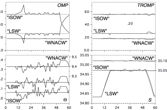
Having identified the most important time-varying property (or properties, ranked in order of importance) it is then possible to proceed with a better targeted TROMP analysis by limiting the number of variables to one or two source water properties for a single SWT. The TROMP algorithm allows us to set limits on the variation of all variables, and the proposed procedure can be implemented by setting extremely narrow (or zero) variation limits for all SWT definitions except the one of interest (in our case LSW salinity). The results of this approach were satisfactory for our first simulated data set, particularly when the analysis was implemented in two or more iterations of stages 1 and 2 for every time step. However, the analysis produced not only the correct time evolution of salinity but also apparent variations in potential temperature, a property that was set to remain constant in the simulated data set (Figure 3).
The problem becomes more acute when the range of SWT variations is small, as in the actual time development of LSW properties, on which we based our second simulated data set. Figure 4 shows the results when TROMP analysis is applied to that data set in the manner just described. It is seen that the analysis traces the actual evolution of LSW potential temperature and salinity closely but contains much unrealistic noise. TROMP analysis improves on the first guesses derived from OMP analysis; it reduces the departure from the correct relative contributions and the noise, but the reduction is rather small.
Figure 4: Results of the analysis of data set 2 for the 1200 m depth level. Variation limits were set to zero for oxygen and nutrients, 3 for LSW temperature and salinity, and 1 for temperature and salinity of all other water masses. Stages 1 and 2 went through 5 iterations at every time step. Relative water mass contributions (%) from the results of stage 1 (OMP analysis, top left) and after five iterations through stages 1 and 2 (TROMP analysis, top right); time development of potential temperature (°C, bottom left) and salinity (bottom right). Thin lines indicate the target values. (At 1200 m the target value for uWNACW is zero).
Fig. 4. Results of the analysis of data set 2 for the 1200 m depth level. Variation limits were set
to zero for oxygen and nutrients, 3 for LSW temperature and salinity, and 1 for temperature and salinity of all other water masses. Stages 1 and 2 went through 5 iterations at every time step. Relative water mass contributions (%) from the results of stage 1 (OMP analysis, top left) and after five iterations through stages 1 and 2 (TROMP analysis, top right); time development of potential temperature (◦C, bottom left) and salinity (bottom right). Thin lines indicate the target values. (At 1200 m the target value for uWNACW is zero).
OSD
2, 399–415, 2005 Remote detection of property changes A. Henry-Edwards and M. Tomczak Title Page Abstract Introduction Conclusions References Tables Figures J I J I Back CloseFull Screen / Esc
Print Version Interactive Discussion
EGU
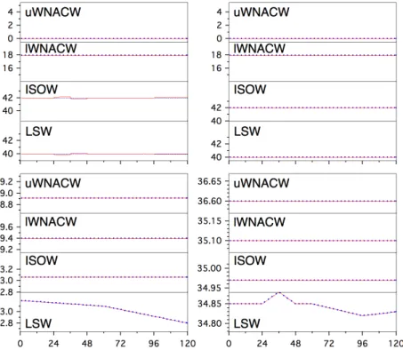
Applying a low-pass filter to the results can of course improve the agreement between observations and analysis. A better way to improve the result can be obtained by restricting the number of variables in the analysis: When all water type properties that are considered unimportant for the explanation of the observed property variations are not handled as variables with extremely narrow variation limits but are declared constants, the TROMP analysis is forced to concentrate on the variable of interest and produces excellent agreement between the simulated data and the results from the analysis (Figure 5).
Figure 5: Results of the analysis of data set 2 for the 1200 m depth level. Oxygen and nutrients were declared constants for all water masses, temperature and salinity for all water masses but LSW. Temperature and salinity of LSW were allowed to vary by up to 3% at every time step. Stages 1 and 2 went through 5 iterations at every time step. Relative water mass contributions (%) from the results of stage 1 (OMP analysis, top left) and after five iterations through stages 1 and 2 (TROMP analysis, top right); time development of potential temperature (°C, bottom left) and salinity (bottom right). Red lines indicate calculated values. Dotted blue lines indicate the target values; where the difference between calculated and target values is not resolved in the graph, the target values are indicated by heavy blue dots. (At 1200 m the target value for uWNACW is zero). Axes are scaled to compare directly with Figure 4.
Fig. 5. Results of the analysis of data set 2 for the 1200 m depth level. Oxygen and nutrients
were declared constants for all water masses, temperature and salinity for all water masses but LSW. Temperature and salinity of LSW were allowed to vary by up to 3% at every time step. Stages 1 and 2 went through 5 iterations at every time step. Relative water mass contributions (%) from the results of stage 1 (OMP analysis, top left) and after five iterations through stages 1 and 2 (TROMP analysis, top right); time development of potential temperature (◦C, bottom left) and salinity (bottom right). Red lines indicate calculated values. Dotted blue lines indicate the target values; where the difference between calculated and target values is not resolved in the graph, the target values are indicated by heavy blue dots. (At 1200 m the target value for uWNACW is zero). Axes are scaled to compare directly with Fig. 4.