HAL Id: hal-02763668
https://hal.inrae.fr/hal-02763668
Submitted on 4 Jun 2020HAL is a multi-disciplinary open access archive for the deposit and dissemination of sci-entific research documents, whether they are pub-lished or not. The documents may come from teaching and research institutions in France or abroad, or from public or private research centers.
L’archive ouverte pluridisciplinaire HAL, est destinée au dépôt et à la diffusion de documents scientifiques de niveau recherche, publiés ou non, émanant des établissements d’enseignement et de recherche français ou étrangers, des laboratoires publics ou privés.
The VENFOR project: a k-e model for simulating wind
flow in heterogeneous forest canopies
Hadjira Foudhil, Yves Brunet, Jean-Paul Caltagirone
To cite this version:
Hadjira Foudhil, Yves Brunet, Jean-Paul Caltagirone. The VENFOR project: a k-e model for sim-ulating wind flow in heterogeneous forest canopies. International Conference Wind Effects on Trees, Sep 2003, Karlsruhe, Germany. �hal-02763668�
International Conference ‘Wind Effects on Trees’
September 16-18, 2003, University of Karlsruhe, Germany
THE VENFOR PROJECT: A k-
ε
MODEL FOR SIMULATING WIND
FLOW IN HETEROGENEOUS FOREST CANOPIES
H. Foudhil1,2, Y. Brunet1 and J.P. Caltagirone2
1. INRA-Bioclimatologie, Bordeaux, France; 2. MASTER-ENSCPB, Talence, France
Abstract
The purpose of this study is to develop a numerical tool for the prediction of turbulent wind flow over heterogeneous terrain in the surface boundary layer. The model is based on the Reynolds equations, averaged in space to consider the interaction with plant canopies. Turbulence is modelled by a k-ε closure scheme, extended by including source-sink terms due to the drag forces on plant elements. The numerical code is validated against a series of data sets from several in-situ and wind-tunnel experiments: smooth-to-rough surface change, wind flow in a horizontally homogeneous canopy, flow over a forest-clearing-forest sequence. The comparison between modelled and measured data show that the model provides adequate simulations in most cases. Some limitations of the model are also shown in regions with strong flow distorsion.
Introduction
In order to understand and predict wind-tree interactions it is of primary importance to be able to simulate the wind flow around trees in various environments. Simple atmospheric flow with fully-developed turbulence over homogeneous terrain can be handled relatively well with simple one-equation (k-l) or two-equation (k-ε) turbulence models. However, real landscapes characterised by surface inhomogeneities (step changes in surface roughness, small topography, forest edges…) are more difficult to deal with because the turbulent flow becomes much more complex in transition regions, where its characteristics strongly depend on upwind and possibly downwind surface features. Nevertheless, the above-mentioned turbulence models may be effective when they are coupled with adequate wall functions and when special care is given to the relevant physical processes. The purpose of this paper is to present a newly-developed k-ε turbulence model adequate for flow within and above plant canopies in transition regions, and validate it against several in-situ and wind-tunnel experimental data sets.
The wind flow model
The model is based on the classical Reynolds equations, on which a spatial average operator has been applied to remove all small-scale horizontal canopy heterogeneities (Raupach and Shaw 1982). Neutral conditions being assumed for this study, the momentum equation can therefore be written as:
> < > >< < − ∂ > < ∂ + ∂ > < ∂ ∂ ∂ + < >+ ∂ ∂ − = ∂ > < ∂ > < + ∂ > < ∂ i j j d i j j i t j i j i j i u u u a C x u x u x k P x x u u t u ρ µ ρ ρ ρ 3 2
where the overbar and the angle brackets refer to time and space averages, respectively; ρ
is the air density, ui the wind component in direction i, P the dynamic pressure, k the
turbulent kinetic energy, µt the eddy viscosity, Cd a drag coefficient and a the frontal area of
plants per unit volume (0 outside of the canopy). In this equation the momentum flux has been assumed proportional to the local gradients in wind velocity, for the sake of simplicity. Using a k-ε model as a turbulence closure scheme, the eddy viscosity is evaluated from the turbulent kinetic energy k and its dissipation rate ε, according to:
ε ρ µt= Cµ k2
where Cµ is an empirical constant.
Two more equations have to be carried out, one for k:
k u u a C C u u a C C P x k x x k u t k j j d w j j d Pw k j k t j j j > >< < − > >< < + − + ∂ ∂ ∂ ∂ = ∂ ∂ > < + ∂ ∂ ε ρ ρ ρε ρ σ µ ρ ρ 2 / 3 ] [
and one for ε:
ε ρ ε ρ ε ρ ε ρ ε σ µ ε ρ ε ρ ε ε ε ε ε > >< < − > >< < + − + ∂ ∂ ∂ ∂ = ∂ ∂ > < + ∂ ∂ j j d w D j j d w P k j t j j j u u a C C u u a C k C k C P k C x x x u t 2 / 3 2 2 1 ] [
where CPw, Cεw, Cε1, Cε2, CPεw and CDεw are empirical constants. Pk is the shear production
rate of kinetic energy, defined as:
j i j i k x u u u P ∂ > < ∂ − = ' '
The 4th term on the r.h.s. of the equation for k is the wake production term P
w, defined as the
product of the mean velocity and the form drag (Green 1992). The 5th term is a wake
dissipation term εw added by Wilson 1988 and Green 1992. In the budget equation for ε the
last two terms have been added to account for the additional role of the canopy in modifying
ε. The value of CPw is taken as 0.8 following Finnigan 2000 and the value of CDεw has been
adjusted to 3.24 in the course of the present work. The values of all other empirical constants are taken from Detering and Etling 1985 and Green 1992. All constants are given in Table 1.
σk σε Cµ Cε1 Cε2 CPw Cεw CPεw CDεw
0.74 1.3 0.0256 1.13 1.9 0.8 4 1.5 3.24
Table 1: Values of the empirical constants used in the flow model.
All boundary conditions are integrated into the equations through additional terms representing surface flux Fourier conditions. At the lower boundary (i.e. at the surface when the canopy is not explicitely considered, or close to the ground under a canopy) standard surface layer laws are used, with a roughness length z0 and a displacement height d. The
vertical gradient of k is assumed to vanish at the wall and an assumption of local equilibrium is used for ε. The upper boundary conditions are representative of a constant flux layer. The discretization grid is dissociated from the geometry considered, with control conditions of the mesh being added to the previous equations as penalization terms. The resulting equations are discretised in time by an implicit scheme, so that no particular stability criterion has to be fulfilled. The velocity-pressure couple is solved by the augmented Lagrangian algorithm. The equations are discretized in space by a finite volume method applied to an irregular staggered Cartesian grid made of a superposition of three grids in two directions. Central differencing and hybrid central/upwind differencing are used to discretize the diffusive and convective terms, respectively. The linear systems resulting from the previous implicit scheme are solved with an iterative bi-conjugate gradient stabilised algorithm.
Change in surface roughness
One first step in the model validation is to check whether it is able to simulate simple transition cases and predict the development of the associated disturbances. This was done using the smooth-to-rough change in surface roughness presented by Bradley 1968. The ratio of roughness lengths between the upstream and downstream regions is 125.
The simulation is carried out by assuming that the incoming flow at the inlet boundary is in equilibrium with the upstream smooth surface. The mean horizontal velocity profile follows a logarithmic law with z01 = 2 10-5 m and a friction velocity u
* = 0.104 m s–1. The transition is set
at x = 0 with z02 = 2.5 10-3 m at the rough surface.
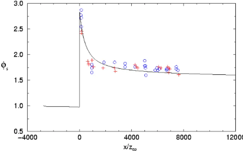
Fig. 1: Variation in normalised surface shear stress downwind of a smooth-to-rough transition (Bradley 1968). Observed (symbols) and modelled (solid lines) values.
Figure 1 shows the observed and computed variation in shear stress across the transition, normalised by its upstream value. At the transition the shear stress increases sharply to a maximum value that is well reproduced by the model. It then decreases asymptotically to its equilibrium value. Throughout the investigated region the agreement between observed and modelled values is good. Other calculations (not shown here) also show a very good prediction of the growth of the internal boundary layer, defined as the height at which the downwind velocity reaches 99% of its upstream value. The height of the simulated constant flux inner layer converges to a classical 0.8 power law of x/z02, reached at x/z02 ≈ 10000.
Flow in homogeneous canopies
A second step in the model validation before considering fully heterogeneous situations is to investigate whether the model is able to simulate the flow in horizontally homogeneous canopies. For this we used the data of Brunet et al 1994, collected during an experiment in an atmospheric wind tunnel designed to simulate wind flow in a fully-developed neutral boundary layer. A flexible roof provides a zero streamwise pressure gradient throughout the working section. The canopy model has a height h = 47 mm, a mean drag coefficient
Cd = 0.675 (omitting the ½ factor) and a vertically uniform plant frontal area per unit volume a = 10 m-1. Triple wires were used for the velocity measurements.
The flow is solved in a two-dimensional domain over a non-uniform rectangular grid of height 0.65 m (the height of the working section), covering the upstream region made of a rough surface (road gravels) and the canopy model. In the vertical direction the mesh size is uniform within the canopy and increases exponentially with height above it. In the horizontal the mesh size is smaller around the transition to the canopy. At the surface standard wall conditions are used (with a very small roughness length at the bottom of the canopy) and at the top of the computational domain Dirichlet type boundary conditions are used for mean horizontal velocity and Neumann type conditions for all other variables.
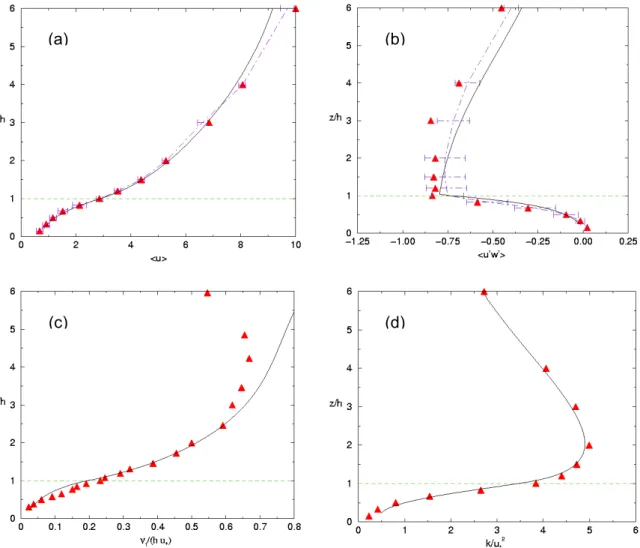
Figure 2 shows comparisons between observed and modelled values for various variables at the farthest downstream position (x = 4.08 m, i.e. x/z0 = 723 or x/h = 87), where the flow has
reached equilibrium. The mean horizontal velocity profile (Fig. 2a) is well simulated throughout the roughness layer and the inertial layer up to about 4 h. Above this height the computed values depart from the measurements, probably because the upper part of the working section is influenced by the streamwise profile of the adjustable roof, not accounted for in the numerical simulations.
Figure 2b shows a comparison of the computed shear stress profile with measured values from a single position (triangles) and from an ensemble average of all collected profiles (dashed line with error bars). The shear stress profile is also well simulated, except that the model fails in reproducing the constant flux layer between about z/h = 1 and 2, visible in the experimental data. In this region the calculated stress slowly decreases (in absolute value) with height. However, the relative change in this layer remains small (less than 8%).
The simulated momentum eddy diffusivity (Fig. 2c) appears surprisingly close to its experimental counterpart up to z/h ≈ 2.5. The flux-gradient relationship, in theory inappropriate to describe turbulent transport in the canopy, holds reasonably well for computational purposes.
(b) (a)
(c) (d)
Fig. 2: Vertical profiles of computed (solid lines) and measured (symbols) values of (a) mean horizontal velocity, (b) shear stress, (c) momentum eddy diffusivity and (d) turbulent kinetic energy. The measured values are taken from the wind-tunnel experiment of Brunet et al 1994.
Finally, Figure 2d shows the turbulent kinetic energy, that appears very well simulated throughout the investigated layer. The dissipation rate (not shown here) is not so well reproduced above the canopy but there is some uncertainty about the experimental values, estimated from the slopes of the u and w spectra (Brunet et al 1994). The profiles of k and ε turn out to be fairly sensitive to the closure constant CDεw.The optimum value (3.24) found
during the course of this work provides both an excellent agreement on k through the whole domain and a good agreement on ε within the canopy.
Flow in heterogeneous canopies
We can now consider heterogeneous canopies, under the form of two-dimensional strips of canopy and smoother surface, perpendicular to the incoming wind. For this we use the data of Raupach et al 1987. Their experiment was carried out in the same wind tunnel as in the previous case, with the same canopy model in which strips had been removed and replaced by a smooth surface made of small gravels. Their set up represents forest-clearing-forest transitions. The present comparison is performed for a clearing of length Lc = 21.3 h. X-wires
Fig. 3: Vertical profiles of computed (solid lines) and measured (symbols) values of mean horizontal velocity at various positions along a forest-clearing-forest transition. The dashed line is the upstream
forest equilibrium model solution. The measured values are taken from the wind-tunnel experiment of Raupach et al 1987.
Figure 3 shows a comparison of computed and measured mean horizontal velocity at 9 positions across the transitions: one in the upstream canopy (x = -2.1 h, x = 0 defining the downwind edge), three in the clearing (x = 2.1, 4.3 and 12.8 h) and five in the downwind
canopy (X = 0, 2.1, 4.3, 6.4 and 10.6 h, X = 0 defining the upstream edge). Over the clearing the model simulates well the streamwise variation in the vertical profiles, although it slightly underestimates the flow acceleration. At the following edge there is good agreement. Further, the model simulates fairly well the decceleration in the canopy and reproduces the inflected profile at all positions downwind. The turbulent kinetic energy (not shown here) is also well simulated, except just after the upstream edge of the downstream canopy (position
X = 2.1 h) where it is too large, i.e. the model fails in reproducing the rapid decrease in
kinetic energy in this region where the flow is strongly distorted. It has to be pointed out that the X-wires used in this experiment are prone to errors in such regions. At the next position (X = 4.3 h) the agreement is good again.
Conclusion
The model presented here provides adequate simulation of the wind flow in simple heterogeneous cases: flow over a smooth-to-rough surface change (where no empirical constant was adjusted) and flow within and above a horizontally homogeneous canopy providing a vertically distributed drag (where one empirical constant appearing in the wake dissipation term of the budget equation for the dissipation rate had to be adjusted). In a more complex situation combining the previous two cases (a canopy-clearing-canopy sequence) the model behaves fairly well but some discrepancies can be observed at several positions, especially in the regions of strong flow distorsion. Further work has to be done on the closure assumptions in such regions, and new data should be acquired during the course of the Venfor project.
Acknowledgements
The GIP Ecofor is gratefully acknowledged for supporting the Venfor project. We also thank INRA and the Région Aquitaine for funding the PhD thesis of H. Foudhil.
References
Bradley, E.F., 1968: "A Micrometeorological Study of Velocity Profiles and Surface Drag in the Region Modified by a Change in Surface Roughness", Quarterly Journal of the Royal Meteorological Society, 94, pp. 361-379.
Brunet, Y., Finnigan, J.J., Raupach, M.R., 1994: "A Wind Ttunnel Study of Air Flow in Waving Wheat: Single-Point Velocity Statistics", Boundary Layer Meteorology, 70, pp. 95-132.
Detering, H.W., Etling, D., 1985: "Application of the E-ε turbulence model to the atmospheric boundary layer", Boundary Layer Meteorology, 33, pp. 113-133.
Finnigan, J.J., 2000: "Turbulence in Plant Canopies", Annual Review of Fluid Mechanics, 32, pp. 519-571.
Green, S.R., 1992: "Modelling Turbulence Air Flow in a stand of Widely-Spaced Trees", Phoenics, Journal of Computational Fluid Dynamics and Applications, 5, pp. 294-312.
Raupach, M.R., Bradley, E.F., Ghadiri, H., 1987: "A Wind Tunnel Investigation into Aerodynamic effect of Forests Clearings on the Nesting of Abbott's Booby on Christmas Island", Internal Report, CSIRO Centre for Environmental Mechanics, Canberra, Australia.
Raupach, M.R., Shaw, R.H., 1982: "Averaging Procedures for Flow within Vegetation Canopies", Boundary Layer Meteorology, 22, pp. 79-90.
Wilson, J.D., 1988: "A second-order closure model for flow through vegetation", Boundary Layer Meteorology, 42, pp. 371-392.
Wilson, J.D., Flesh, T., 1999: "Wind and Remnant Tree Sway in Forest Cutblocks. III. A Windflow Model to Diagnose Spatial Variation", Agricultural and Forest Meteorology, 93, pp. 259-282.