The effect of composition on the boiling rates of liquefied natural gas for confined spills on water

OF LIQUEFIED NATURAL GAS FOR CONFINED SPILLS ON WATER

by

Jaime A. Yalencia-Chavez

B.S., University of Maryland (December, 1973)

Submitted in Partial Fulfillment of the Requirements for the

Degree of Doctor of Science

at the

MASSACHUSETTS INSTITUTE OF TECHNOLOGY February, 19781

Signature of Author:

Certified by:

Accepted by:

DepartS" of Chei'ical En§geering

Professor R. C. Reid Thesis Superviso - _

Chairman, Departmental Committee on ARCHIVES Graduate Theses

MAR

13

1978

"t~*,t~_~~a99a

THE EFFECT OF COMPOSITION ON THE BOILING RATES OF LIQUEFIED NATURAL GAS FOR CONFINED

SPILLS ON WATER

by

Jaime A. Valencia-Chavez

Submitted to the Department of Chemical Engineering on February 14, 1978, in partial fulfillment of the

requirements for the degree of Doctor of Science.

The effect of composition on the boiling rates for confined spills of LNG on water was studied. Addition of heavier hydrocarbons to pure methane changed the boiling rates significantly, specifically increasing them in the initial period of time, thus leading to a higher maximum heat flux.

Upon contact with water, a preferential evaporation of the more volatile components takes place. The composition of the vapors evolved, as well as the temperature of the residual LNG, were experimentally determined at various times after the spill. Predictions made for the vapor composition and saturation temperature based on vapor-liquid equilibria considerations agreed well with the experimental data.

Initially, LNG mixtures film boil on water. A theory has been developed for the collapse of this film resulting in the high heat fluxes and boiling rates observed in the initial period. Consideration

is given to the rise in saturation temperature following the depletion of methane, as well as to the amount of energy required to warm the residual LNG to this rising temperature.

Based on the above considerations, a heat transfer model that

draws information from the vapor-liquid equilibria model has been devel-oped. This combined heat transfer/vapor-liquid equilibria model predicts

successfully the evaporation of confined spills of LNG on water.

Thesis Supervisor: Robert C. Reid

Department of Chemical Engineering Massachusetts Institute of Technology Cambridge, Massachusetts 01239

February, 1978

Professor Irving Kaplan Secretary of the Faculty

Massachusetts Institute of Technology Cambridge, Massachusetts 02139

Dear Professor Kaplan:

In accordance with the regulations of the Faculty, I herewith submit a thesis, entitled "The Effect of Composition on the Boiling Rates of Liquefied Natural Gas for Confined Spills on Water," in partial fulfillment of the requirements for the degree of Doctor of Science in Chemical Engineering at the Massachusetts Institute of Technology.

Respectfully submitted,

To my parents Luis and Julia

ACKNOWLEDGEMENTS

Generally a doctoral thesis represents a painstaking process and quite often difficult times. I would like to thank my thesis supervisor Professor Robert C.Reid; his encouragement and enthusiasm not only

reduced the difficulties, they almost made it fun to work on this thesis. I would also like to express my gratitude to the members of my thesis committee, Professors T. Drew, W. Rohsenow and K.A. Smith for their technical comments.

To my friends in the Department, too numerous to mention all of them here, go my thanks for their help in the many facets of my work, but mostly for their friendship. In particular, I would like to thank Kenton Griffis and Ross Wilcox for their technical suggestions. Most of all I am indebted to Mary Jane Garry who not only helped me through

the rough spots but also labeled all of my graphs, edited and proof-read the thesis.

Finally I would like to thank Debbie Hackel for typing the manuscript.

TABLE OF CONTENTS

I. Summary 21

Introduction 21

Experimental 25

Vapor-Liquid Equilibria 29

Development of the VLE Model 30

Results 34

Boiling of LNG on Water 35

Results 38

Discussion of Results 43

Heat Transfer Models 46

Regression of Surface Temperatures by Using 46 Convolution Integrals

Variable Grid Size Heat Transfer Model 50

Conclusions 56

II. Previous Work Relevant to the Boiling of LNG on Water 58

Regimes of Boiling 58

Effect of Surface Roughness on Pool Boiling 60

Boiling of Liquid-Liquid Interfaces 65

Boiling Heat Transfer to Liquid Mixtures 68 Boiling of Cryogenic Liquids on Solid Surfaces 75 Boiling of Cryogenic Fluids on Water 86

III. Experimental 107

Equipment for Spills of LNG on Water 107

Preparation of Cryogens 114

Analysis of Chemical Composition 117

IV. Vapor-Liquid Equilibria 121

Introduction 121

Deveaipment cf the VLE Mcdel 122

Applicability of the SRK Equation of State 133

Experimental Vapor Sampling 145

TABLE OF CONTENTS - cont. V. Boiling of LNG on Water 173 Results 173 Methane 173 Ethane 178 Propane 182 Nitrogen 186 Methane-Ethane Mixtures 187 Ethane-Propane Mixtures 191 Methane-Ethane-Propane Mixtures 191

Mixtures Containing Nitrogen 206

Water Temperatures 212 Vapor Temperatures 212 Discussion of Results 213 Methane 213 Ethane 218 Propane 220 Mixtures 221 Comparison of Results 227

VI. Heat Transfer Models 230

Previous Models 230

Semi-Infinite Solid 236

Moving Boundary Model 245

Regression of Surface Temperature by Using 255 Convolution Integrals

Boiling on Ice 255

Boiling on Water 261

Variable Grid Size Heat Transfer Model 270 Combined VGS/VLE HTM Model for LNG Mixtures 279 VII. Secondary Observations Regarding the Evaporation of 300

Light Hydrocarbons on Water

Foaming 300

Solid PhZac (ice) Ccmposition 304

TABLE OF CONTENTS - cont. VIII. Conclusions and Recommendations

Conclusions Recommendations Appendices

A. Experimental

Electronic Balance Real Time Computer Computer Programs to Thermocouples

Gas Chromatograph

Monitor Data Acquisition

B. Vapor-Liquid Equilibria

The Soave-Redlich-Kwong Equation

Determination of the SRK Interaction Parameters, k.. Logic Diagram: Evaluation of Residual Liquid Compositi Vapor Sampling Time

Computer Programs

C. Computation of Boiling Rates Procedure

Computer Programs D. Heat Transfer Models

Properties of Ice Properties of Water Computer Programs

Convolution Integral

Variable Grid Size Heat Transfer Model VGS/VLE HTM Bibliography 313 313 316 317 317 318 324 327 334 339 342 343 347 on 357 359 361 379 380 382 392 393 394 395 395 403 408 421

TABLE OF CONTENTS Location of Original Data

Biographical Note

- cont.

427 428

LIST OF FIGURES

1-1 Experimental Set-up for the Study of LNG Boiling on 27 Water

1-2 Boiling Vessel 28

1-3 Pressure Composition Diagram for the Methane-Ethane 33 System (kij = 0.0)

1-4 Vapor Composition as a Function of Mass Evaporated 36 (85.2% Methane, 10.1% Ethane, 4.7% Propane)

1-5 Temperature as a Function of Mass Evaporated (85.2% 37 Methane, 10.1% Ethane, 4.7% Propane)

1-6 Mass Evaporated for Methane Boiling on Water 39

1-7 Boiling Rates for Methane 40

1-8 Mass Evaporated for Run R-20, Ternary Mixture 41 1-9 Boiling Rates for Run R-20, Ternary Mixture 42 1-10 Drop in Surface Temperature of Ice after a Methane 48

Spill

1-11 Drop in Surface Temperature of Ice after a Spill of 49 Methane on Water

1-12 Boiling of a Methane-Ethane Mixture on Water (R-1). 52 VGS/VLE HTM Predictions and Experimental Data

('cf = 25 s)

1-13 Evaporation Rates of a Methane-Ethane Mixture on 53 Water (R-1). VGS/VLE HTM Predictions and Experimental

Data (Tcf = 25 s)

1-14 Boiling of a Methane-Ethane-Propane Mixture on Water 54 (R-20). VGS/VLE HTM Predictions and Experimental

Data (cf = 5 s)

1-15 Evaporation Rates of a Methane-Ethane-Propane Mixture 55 on Water (R-20). VGS/VLE HTM Predictions and

LIST OF FIGURES - cont.

2-1 Regimes of Boiling 61

2-2 Effect of Surface Conditions on Boiling Heat Transfer 62 2-3 Effect of Roughness on Boiling Characteristics. 64

Pentane Boiling on Copper (Berenson, 1962)

2-4 Effect of Heating Surface on the Nucleate Boiling of 67 Pentane

2-5 Peak Nucleate Heat Fluxes for Water-Methyl Ethyl Ketone 69 Mixtures (Van Wijk, 1956)

2-6 Peak Nucleate Heat Fluxes for Water-l-Pentanol Mixtures 70 (Van Wijk, 1956)

2-7 Boiling of Liquid Nitrogen on Solid Surfaces at 76 Atmospheric Pressure

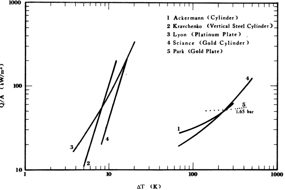
2-8 Boiling of Methane on Solid Surfaces at Atmospheric 78 Pressure

2-9 Boiling of Ethane on a Gold Plated Surface at Atmospheric 80 Pressure

2-10 Boiling of LNG and Methane on a Gold Plated Surface at 81 Atmospheric Pressure

2-11 Boiling of LPG and Propane on a Gold Plated Surface at 83 Atmospheric Pressure

2-12 Effect of Composition on AT for Propane-n-Butane Mixtures 84 at a Reduced Pressure of 0.3 - or 12.7 bar - (Clements,

1973)

2-13 Effect of Composition on Nucleate Boiling of Propane- 85 n-Butane Mixtures, Pr = 0.3 (Clements, 1973)

2-14 Effect of LNG Composition on Evaporation Rate 91 (Boyle and Kneebone, 1973)

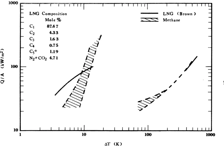
2-15 Boiling of Methane and LNG on Gold and Water 94 2-16 Effect of Addition of Heavier Hydrocarbons on the 98

Boiling of Methane on Water (Jeje, 1974)

2-17 Effect of Composition on the Boiling Heat Transfer of 100 LNG on Water (Jeje, 1974)

LIST OF FIGURES - cont.

3-1 Experimental Set-up for the Study of LNG Boiling on Water

3-2 Boiling Vessel 3-3 Cryogen Distributor

3-4 Temperature Measurement. a) Vapor Thermocouple

b) Typical Locations of Vapor and Liquid Thermocouples 3-5 Methane Liquefaction Apparatus

3-6 Ethane and Propane Liquefaction Apparatus

3-7 Sampling Bulb and Scoop for Chromatographic Analysis

4-1 Logic Diagram to Insure a Value of AL 5 0.01 Moles is Used Throughout the VLE Model

4-2 Pressure Composition Diagram for System (kij = 0.0)

4-3 Pressure Composition Diagram for System. Low Pressure Range (kij 4-4 Pressure Composition Diagram for

(kij = 0.01)

4-5 Pressure Composition Diagram for System (kij = 0.0)

4-6 Pressure Composition Diagram for System (kij = 0.035)

4-7 Pressure Composition Diagram for System (kij = 0.035) 108 110 112 113 115 115 119 132 134 135 137 138 139 140 141 147 149 152 the Methane-Ethane the Methane-Ethane = 0.0) Methane-Propane System the Ethane-Propane the Nitrogen-Methane Nitrogen-Ethane 4-8 Pressure Composition Diagram for the Nitrogen-Propane

System (kij = 0.120) 4-9 Vapor Sampling Bulb

4-10 Schematic of the Vapor Sampling Procedure

4-11 Temperature Composition Diagram for the Methane-Ethane System

LIST OF FIGURES - cont.

4-12 Temperature Composition Diagram for the Ethane-Propane 154 System

4-13 Temperature Composition Diagram for the Methane- 155 Propane System

4-14 Vapor Composition as a Function of Mass Evaporated 156 (83.5% Methane, 16.5% Ethane)

4-15 Vapor Composition Composition as a Function of Mass 157 Evaporated (89.7% Ethane, 10.3% Propane)

4-16 Temperature as a Function of Mass Evaporated (89.7% 158 Ethane, 10.3% Propane)

4-17 Vapor Composition as a Function of Mass Evaporated 160 (84.0% Methane, 9.4% Ethane, 6.6% Propane)

4-18 Temperature as a Function of Mass Evaporated (84.0% 161 Methane, 9.4% Ethane, 6.6% Propane)

4-19 Vapor Composition as a Function of Mass Evaporated 162 (88.9% Methane, 10.2% Ethane, 0.9% Propane)

4-20 Temperature as a Function of Mass Evaporated (88.9% 163 Methane, 10.2% Ethane, 0.9% Propane)

4-21 Vapor Composition as a Function of Mass Evaporated 164 (83.9% Methane, 8.1% Ethane, 8.0% Propane)

4-22 Temperature as a Function of Mass Evaporated (83.9% 165 Methane, 8.1% Ethane, 8.0% Propane)

4-23 Vapor Composition as a Function of Mass Evaporated 166 (51.8% Methane, 30.0% Ethane, 18.2% Propane)

4-24 Vapor Composition as a Function of Mass Evaporated 167 (70.1% Methane, 20.5% Ethane, 9.4 Propane)

4-25 Temperature as a Function of Mass Evaporated (70.1% 168 Methane, 20.5 Ethane, 9.4% Propane)

4-26 Vapor Composition as a Function of Mass Evaporated 169 (85.2% Methane, 10.1% Ethane, 4.7% Propane)

4-27 Temperature as a Function of Mass Evaporated (85.2% 170 Methane, 10.1% Ethane, 4.7% Propane)

LIST OF FIGURES - cont.

4-28 Vapor Composition as a Function of Mass Evaporated 171 (91.0% Methane, 6.5% Ethane, 2.5% Propane)

4-29 Temperature as a Function of Mass Evaporated (91.0% 172 Methane, 6.5% Ethane, 2.5% Propane)

5-1 Mass Evaporated for Methane Boiling on Water 175

5-2 Boiling Rates for Methane 177

5-3 Mass Evaporated for Ethane Boiling on Water 180

5-4 Boiling Rates for Ethane 181

5-5 Mass Evaporated for Propane Boiling on Water 184

5-6 Boiling Rates for Propane 185

5-7 Mass Evaporated for Methane-Ethane Mixtures Boiling 189 on Water

5-8 Boiling Rates for Methane-Ethane Mixtures 190 5-9 Mass Evaporated for Ethane-Propane Mixtures Boiling 193

on Water

5-10 Boiling Rates for Ethane-Propane Mixtures 194 5-11 Mass Evaporated for Run R-15, Ternary Mixture 196 5-12 Boiling Rates for Run R-15, Ternary Mixture 197 5-13 Mass Evaporated for Run R-20, Ternary Mixture 198 5-14 Boiling Rates for Run R-20, Ternary Mixture 199 5-15 Mass Evaporated for Run R-37, Ternary Mixture 200 5-16 Boiling Rates for Run R-37, Ternary Mixture 201 5-17 Mass Evaporated for Run R-41, Ternary Mixture 202 5-18 Boiling Rates for Run R-41, Ternary Mixture 203 5-19 Mass Evaporated for Run R-64, Ternary Mixture 204

LIST OF FIGURES - cont.

5-20 Boiling Rates for Run R-64, Ternary Mixture 205 5-21 Mass Evaporated for Methane-Nitrogen Mixtures Boiling 208

on Water

5-22 Boiling Rates for Methane-Nitrogen Mixtures 210 5-23 Mass Evaporated for Methane-Ethane-Propane-Nitrogen 211

Mixtures

5-24 Mass Evaporated for Methane Boiling on Water and on Ice 217 5-25 Mass Evaporated for Ethane Boiling on Water and on Ice 219 5-26 Mass Evaporated for Propane Boiling on Water and on Ice 222 5-27 Sequence of Events leading to the Collapse of the Vapor 225

Film During Boiling of a Methane Ethane Mixture

6-1 Comparison of Previous Models for Evaporation of LNG on 232 Water with Experimental Data

6-2 Comparison of Previous Models for Evaporation Rates of 233 LNG on Water with Experimental Data

6-3 Semi-Infinite Solid Model 238

6-4 Boiling of Methane on Ice. Semi-Infinite Solid Model 242 and Experimental Data

6-5 Boiling of Ethane on Ice. Semi-Infinite Solid Model 243 and Experimental Data

6-6 Boiling of Propane on Ice. Semi-Infinite Solid Model 244 and Experimental Data

6-7 Moving Boundary Model 246

6-8 Boiling of Methane on Water. Moving Boundary Model 252 and Experimental Data

6-9 Boiling of Ethane on Water. Moving Boundary Model 253 and Experimental Data

6-10 Boiling of Propane on Water. Moving Boundary Model 254 and Experimental Data

LIST OF FIGURES - cont.

6-11 Drop in Surface Temperature of Ice after a Methane Spill 259 6-12 Drop in Surface Temperature of Ice after an Ethane Spill 260 6-13 Drop in Surface Temperature of Ice after a Spill of 262

Methane on Water

6-14 Drop in Surface Temperature of Ice after a Spill of 263 Ethane on Water

6-15 Transient Boiling of Methane on Water Compared to 265 Steady State Boiling on Metal Surfaces

6-16 Transient Boiling of Ethane on Water Compared to 266 Steady State Boiling on Metal Surfaces

6-17 Transient Boiling of a Methane-Ethane Mixture on Water 268 6-18 Transient Boiling of an LNG Mixture (C₁ 82.5%, C2 13.1%, 269

C3 4.4%) Compared to Steady State Boiling of LNG

(C₁ 87.5%, C₂ 4.3%, C3 1.6%, C4 +/N2/CO2 6.6%) on a

Metal Surface

6-19 Variable Grid Size Scheme 272

6-20 Boiling of Methane on Water. Variable Grid Size Heat 277 Transfer Model and Experimental Data (Tcf = 45 s)

6-21 Evaporation Rates of Methane Boiling on Water. Variable 278 Grid Size Heat Transfer Model and Experimental Data

(Tcf = 45 s)

6-22 Boiling of Ethane on Water. Variable Grid Size Heat 280 Transfer Model and Experimental Data ( cf = 13 s)

6-23 Evaporation Rates of Ethane Boiling on Water. Variable 281 Grid Size Heat Transfer Model and Experimental Data

(Tcf = 13 s)

6-24 Variable Grid Size/Vapor Liquid Equilibria Heat 282 Transfer Model (VGS/VLE HTM)

6-25 Times for Collapse of Vapor Film (Tcf) for Binary 284 Methane-Ethane Mixtures

LIST OF FIGURES - cont.

6-26 Boiling of a Methane-Ethane Mixture on Water (R-l). 286 VGS/VLE HTM Predictions and Experimental Data

(Tcf = 25 s)

6-27 Evaporation Rates of a Methane-Ethane Mixture on 287 Water (R-l). VGS/VLE HTM Predictions and Experimental

Data (Tcf = 25 s)

6-28 Boiling of a Methane-Ethane Mixture on Water (R-17). 288 VGS/VLE HTM Predictions and Experimental Data

(Tcf = 25 s)

6-29 Evaporation Rates of a Methane-Ethane Mixture on Water 289 (R-17). VGS/VLE HTM Predictions and Experimental Data

(Tcf = 13 s)

6-30 Boiling of a Methane-Ethane Mixture on Water (R-35). 290 VGS/VLE HTM Predictions and Experimental Data

(Tcf = 11 s)

6-31 Evaporation Rates of a Methane-Ethane Mixture on Water 291 (R-35). VGS/VLE HTM Prediction and Experimental Data

(-cf = 11 s)

6-32 Boiling of an Ethane-Propane Mixture on Water (R-30). 292 VGS/VLE HTM Predictions and Experimental Data

(Tcf = 5 s)

6-33 Evaporation Rates of an Ethane-Propane Mixture on 293 Water (R-30). VGS/VLE HTM Predictions and Experimental

Data (rcf = 5 s)

6-34 Boiling of an LNG Mixture on Water (R-15). VGS/VLE HTM 294 Predictions and Experimental Data (Tcf = 5 s)

6-35 Evaporation Rates of an LNG Mixture on Water (R-15). 295 VGS/VLE HTM Predictions and Experimental Data

(TC = 5 s)

6-36 Boiling of an LNG Mixture on Water (R-20). VGS/VLE HTM 296 Predictions and Experimental Data (Tcf = 5 s)

6-37 Evaporation Rates of an LNG Mixture on Water (R-20). 297 VGS/VLE HT:I Prdictions and Experimental Data

LIST OF FIGURES - cont.

6-38 Boiling of an LNG Mixture on Water (R-41). VGS/VLE HTM 298 Predictions and Experimental Data (Tcf = 10 s)

6-39 Evaporation Rates of an LNG Mixture on Water (R-41). 299 VGS/VLE HTM Predictions and Experimental Data

('cf = 10 s)

A-1 Block Diagram for the METTLER P11 Electronic Balance 319 A-2 Response Time of the Balance, 128 g Dropped from 5 cm 322 A-3 Response Time of the Balance, 1000 g Dropped from 2.5 cm 322 A-4 Response Time of the Balance, 128 g Dropped from 18 cm 323 A-5 Response Time for a 25 im Thick, 2.3 cm Long Ribbon 337

Thermocouple

A-6 Response Time for 150 pm Thick, 0.2 cm Long Lead 337 Thermocouple

A-7 Response Time of a 150 pm Thick, 0.3 cm Long Lead 338 Thermocouple. Base of Leads in 308 K Water and Leads

in Liquid Nitrogen

B-1 Effect of the Interaction Parameter on the Accuracy of 348 VLE Predictions by the SRK Equation. Methane-Ethane

System

B-2 Effect of the Interaction Parameter on the Accuracy of 350 VLE Predictions by the SRK Equation. Methane-Propane

System

B-3 Effect of the Interaction Parameter on the Accuracy of 352 SRK Predictions. Ethane-Propane System

B-4 Flow Chart to Insure a Value of AL 0.01 Moles is 358 Used Throughout the VLE Model

LIST OF TABLES

Burgess' Results for Boiling of Cryogenic Fluids Boiling of Nitrogen on Water

Boiling of Liquid Methane on Water Boiling of LNG on Water 87 103 104 105 126 130 142 146 4-1 Binary Interaction Parameter, kij, for the SRK Equation

4-2 Hypothetical Evaporation of a Hydrocarbon Mixture Using Various Mole Decrements

4-3 Comparison of SRK Predictions for Pressure and Vapor Composition with Experimental Data by Price and Kobayashi. Methane-Ethane-Propane System (283 K) 4-4 Comparison of SRK Predictions for Pressure and Vapor

Composition with Experimental Data by Price and Kobayashi. Methane-Ethane-Propane System (172 K) 4-5 Experimental VLE Model 5-1 Experimental 5-2 Experimental 5-3 Experimental 5-4 Experimental 5-5 Experimental 5-6 Experimental Mixtures 5-7 Experimental Nitrogen

Conditions for LNG Spills Related to the

Conditions Conditions Conditions Conditions Conditions Conditions

for Methane Spills for Ethane Spills for Propane Spills

for Methane-Ethane Mixtures for Ethane-Propane Mixtures for Methane-Ethane-Propane Conditions for Mixtures Containing 5-8 Isothermal Vapor Pressures for Methane-Ethane

Mixtures (113 K)

5-9 Boiling of Liquid Methane on Water 2-1 2-2 2-3 2-4 151 174 179 183 188 192 195 207 223 229

LIST OF TABLES - cont.

6-1 Thermophysical Properties Used in the Semi-Infinite 240 Solid Model

6-2 Thermophysical Properties Used in the Moving Boundary 250 Model

7-1 Analysis of Ice for Presence of Hydrocarbons 307 A-1 Performance and Design Specifications for the Electronic 320

Balance

A-2 Input Ranges Available for the Multi-Range Analog Input 325 Modules

A-3 Retention Times in Chromatographic Analysis 340 B-1 Effect of the Interaction Parameter, k.W on the 349

Accuracy of VLE Predictions by the SRK Equation. Methane-Ethane System

B-2 Effect of the Interaction Parameter, ki, on the 351 Accuracy of VLE Predictions by the SRK Equation.

Methane-Propane System

B-3 Effect of the Interaction Parameter, k., on the 353 Accuracy of VLE Predictions by the SRK Equation.

Ethane-Propane System

B-4 Effect of the Interaction Parameter, kij, on the 354 Accuracy of VLE Predictions by the SRK Equation.

Nitrogen-Methane System

B-5 Effect of the Interaction Parameter, kij, on the 355 Accuracy of VLE Predictions by the SRK Equation.

Nitrogen-Ethane System

B-6 Effect of the Interaction Parameter, ki, on the 356 Accuracy of VLE Predictions by the SRK Equation.

I. SUMMARY

Introduction

The supply of fuels in the USA decreased in the recent past. As a consequence, increasing amounts of LNG may be imported to meet the demand for energy. Questions have been raised, by both public and private interests, regarding the safety of the marine transporta-tion of LNG. A collision involving an LNG tanker or a failure in the loading/unloading system could result in the accidental spillage of LNG on water. LNG is a mixture of methane, some ethane, small amounts of propane and traces of heavier hydrocarbons. It is usually trans-ported at a temperature near its normal boiling point ("115 K) and close to atmospheric pressure. When LNG contacts a hot surface, water, at a higher temperature than its saturation temperature, it will boil and form a hydrocarbon vapor cloud. This cloud when mixed with air could form a flammable mixture.

As part of safety evaluation programs, several studies (Burgess, 1970, 1972; Boyle and Kneebone, 1973; Vestal, 1973; Jeje, 1974) were made to determine the rates of evaporation of LNG on water and the factors that influence such rates.

Burgess used an aquarium which was placed on a load cell. About 19 liters of water were placed in the aquarium and 4 to 8 liters of cryogen were spilled on it. As the cryogen evaporated, the time for each 50 g loss was recorded. For the first 20-40 seconds, the boiling

rate of LNG was reported to be relatively constant with an average value of 0.018 g/cm2-s. The maximum observed rate of evaporation was

0.030 g/cm2-s, 65% higher than the average value. The aquarium was later replaced by a polystyrene ice chest (1972). The reported

boiling rates for the first 20 seconds were 0.015 g/cm2-s. No expla-nation was given for the discrepancy with the value reported in 1970. The boiling rates were found to decrease after ice formation took place on the water surface.

Similar spills using pure methane yielded boiling rates ranging from 0.010 to 0.016 g/cm2-s. The higher value corresponds to a spill twice the amount of that represented by the lower rate. The boiling rates of methane were reported to have increased with time.

The higher boiling rate exhibited by LNG when compared to methane was believed to be due to the exothermic formation of hydrates. This idea, however, was abandoned after measuring rates of hydrate forma-tion; they were much too slow to account for the difference in boiling rate.

Boyle and Kneebone (1973) performed LNG evaporation experiments both on confined and unconfined pools of water. The restricted area experiments were carried out on tanks, 0.836 m2 and 3.72 m2 , placed on a load cell. It was found that boil-off rates increased with time reaching a maximum at the point of "pool break-up". This point is attained when the amount of LNG is no longer sufficient to cover completely the water surface. Evaluation of the LNG layer thickness at pool break-up yielded a value of 1.8 mm for many experiments.

The maximum rate observed in any one experiment was 0.02 g/cm2-s. An increase in the initial quantity of LNG spilled was reflected in

an increase in boil-off rate. Interestingly enough, for a very large spill, the evaporation rate reached a maximum of 0.02 g/cm2_{-s, and}

then declined even though the water was still completely covered with LNG. Decreasing the initial water temperature also caused an increase in boiling rate.

Boyle and Kneebone found a strong dependence of evaporation rate on the chemical composition of the LNG. Increasing the amount of

heavier hydrocarbons such that the methane fraction dropped from 0.99 to 0.95 caused a threefold increase in the rate of evaporation. The following explanation was given for these results. As LNG is spilled on water, the large temperature difference causes film boiling. Heat is supplied by cooling a thin layer of water. Once this layer reaches the freezing point of water, ice forms and cools down very fast. The temperature difference between the ice surface and the LNG decreases enormously; nucleate boiling is promoted thereby causing a rise in heat flux and evaporation rate with time.

Although Boyle and Kneebone's explanation for the observed rates is a very logical one, their data cannot be completely trusted. Most of the spills corresponded to an equivalent non-boiling hydrostatic head of only 0.4 to 0.6 cm, barely 2 to 3 times the pool break-up thickness of 0.18 cm. Furthermore, these spills were carried out on large water surfaces of 3700 and 8400 cm2 (4 and 9 ft2). Since the volumes spilled were relatively small, the spreading effects become significant and should be accounted for, but they were not.

Vestal (1973) used a glass Dewar flask coupled to a load cell to study the heat transfer between cryogenic liquids and water. The maximum rates of evaporation were reported to be 0.04 g/cm2 for pure methane and 0.11 g/cm2 for LNG. These values are considerably higher

than those given by Burgess and by Boyle and Kneebone. The flask used by Vestal had an inside diameter of only 48 mm. Thus, a signi-ficant amount of heat is believed to have been supplied by the cooling of the thick glass walls of the flask.

Jeje (1974) studied the transient boiling of light liquid hydro-carbons on water. Liquid methane and liquid ethane did not show much sensitivity to the amount spilled nor to the initial water temperature. Ice formation took place for both hydrocarbons, although in the case of ethane it formed more rapidly.

The heat fluxes for ethane were higher than those observed for methane. The boil-off rate of methane increased continuously with

time, whereas ethane started boiling slowly and then rapidly increased. Addition of heavier hydrocarbons increased the boiling rate of methane significantly. After 10 seconds, the mass evaporated for mixtures of methane containing 1.6 mole percent ethane and 0.1 mole

percent propane, was twice that for pure methane. For mixtures con-taining 8.2% ethane and 2.0% propane, the mass evaporated after 10 seconds was nearly three times that for pure methane.

The boiling rates for LNG mixtures increased with time and decreased slightly with increased initial water temperature.

The most important conclusion that can be reached after reviewing previous research efforts is that the chemical composition of the LNG plays the most important role in determining the boiling behavior of the mixture. Only qualitative explanations had been offered which are

not completely satisfactory. No attempts were made to explain quantitatively the boiling of LNG on water.

Determination of boiling rates of LNG spilled on open sea is extremely difficult. There are no techniques available for accurately determining these rates. So far, any attempts to measure these rates

have been based on aerial observation of the LNG pool area as a function of time. In addition to the composition of LNG, two other factors play an important role in the evaporation of LNG on the open sea:

the spreading of the LNG pool and the wave motion of the water. Before these effects can be incorporated in a scheme to predict the boiling rates, one must have a clear understanding of how the composition affects the boiling of LNG on water. Furthermore, one must be able to quantify these effects. Such has been the goal of this study.

Experimental

The spillage of LNG on water results in a highly transient process of evaporation. In order to study the characteristics of this process, one must be able to measure, or otherwise determine, the mass evapor-ated, the composition of the liquid and vapor, and the system temper-atures as a function of time. In the present work this was accomplished by spilling the cryogen on quiescent distilled water contained in a

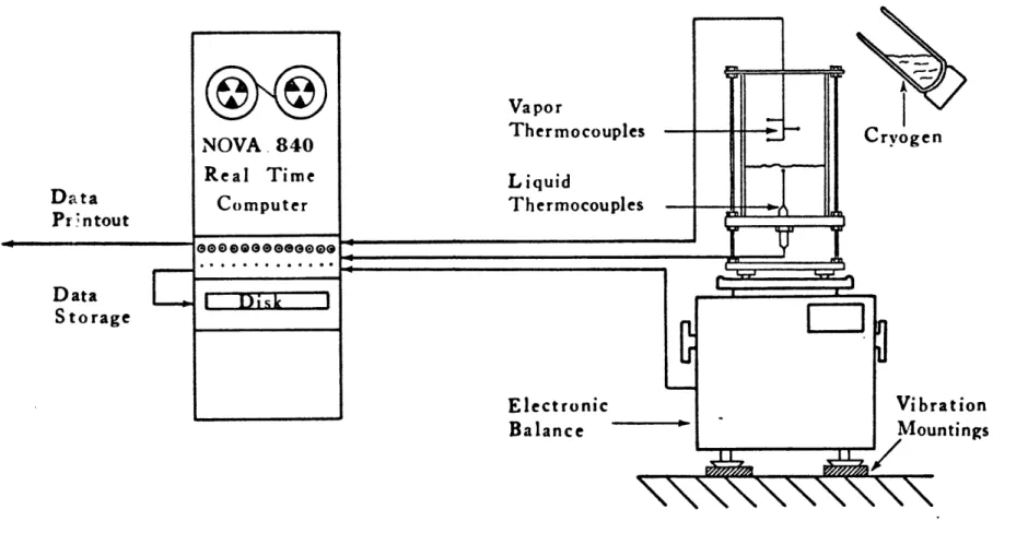
boiling vessel placed on an electronic balance. The output of this balance was monitored by a NOVA-840 real time computer. Water, cryogen, and vapor temperatures were measured by thermocouples whose output was also fed into the real time computer. A schematic repre-sentation of this setup is given in Figure 1-1.

The boiling vessel, shown in Figure 1-2, was a triple wall

cylindrical container. It was transparent to allow visual observation and was designed to minimize heat leaks. The outer wall was made of 0.32 cm thick acrylic tube; the inner walls were made of 25 pm Mylar sheets. The three walls were separated by 2 mm thick polyurethane spacers. These spacers were wound horizontally and were positioned at different heights around the walls. They not only kept the thin walls

in place but minimized natural convection of the air present within the wall gaps.

In most spills the cryogen evaporated completely within 2 to 3 minutes. In this short period of time the most important heat leaks

are due to the cooling of the walls of the container and, therefore, it was necessary to use very thin inner walls to minimize their thermal mass.

A cryogen distributor was used to reduce disturbances to the water surface, and to prevent overshoots on the mass recorded by the

balance due to the inertia of the cryogen spilled.

Three vapor thermocouples were fed through the steel tube guide for the cryogen distributor. The first thermocouple was placed about 2 cm above the cryogen surface; the other two were placed at 1.5 cm

NOVA 840 Real Time Computer e000eeeeee000

I Disk

Figure 1-1 Experimental Set-up for the Study of LNG Boiling on Water

Data Printout

Data

Distributor Guide Acrylic Wall-Vapor Thermocouple Assembly Cryogen Water Liquid Thermocouples Mylar Walls Cryogen Distributor Foam Spacer Supporting Rods Horizontal -Level Adjustment

intervals above the first one. Six liquid thermocouples were used to monitor water and LNG temperatures.

In general, the liquid hydrocarbons were prepared by cooling the hydrocarbon gases below their boiling point either with liquid nitrogen or with a pentane-nitrogen slush bath.

The composition of the hydrocarbon mixture was determined by two methods: gravimetric and chromatographic. The gravimetric method

consisted of accurately weighing the amount of each component added to the mixture. For the chromatographic method, a sample of the liquid mixture was removed with a pre-cooled sampling scoop and introduced

into a sampling bulb. After the liquid evaporated, a sample was removed and analyzed with a gas chromatograph.

Vapor-Liquid Equilibria

LNG is a cryogenic fluid comprised of components which differ significantly in volatility. Thus, in a transient boiling experiment, the vapor evolved varies in composition as the liquid becomes enriched in the less volatile components. This time-dependent vapor composition would show a maximum in nitrogen, if present, followed by methane,

ethane, propane, etc. It is important to be able to estimate the composition of the vapor during a spill of LNG because each component may affect the dispersion characteristics of the cloud. It is also

important to estimate the liquid composition since the saturation

temperature of the residual liquid depends on its composition. Changes in the saturation temperature could significantly affect the heat

One could assume that vapor-liquid equilibrium existed at all times; the vapor composition could then be computed as a function of the

residual liquid composition. Before proceeding with this assumption, however, it is imperative to demonstrate its validity. To this end

the vapor composition was measured experimentally as a function of time and compared with results obtained from theory assuming vapor-liquid equilibria. In addition, temperature measurements in both the liquid and vapor are compared with those predicted from theory.

Pevetopment o6 the VLE Model

For a mixture at thermodynamic equilibrium, the fugacity coefficients i can be related to pressure, total volume and temperature by the

following thermodynamic relationship (Prausnitz et al., 1967)

ln i = In yip 1 RT TVdV - In Z (1-1)

where n. = number of moles of component i Z = PV/nT RT

The Soave (1972) modification of the Redlich-Kwong (1949) equation of state (SRK)

RT a _(1-2)

v - b v;v + b) where v = molar volume

a = temperature dependent term b = constant

can be used to relate pressure, temperature and volume. Thus the fugacity coefficients can be evaluated by combining Eqs. (1-1) and (1-2), b. Ab (1-k. )(a 0

1

k.. = binary interaction parameter

13

To determine the values of the interaction parameters, only binary equilibrium data are required. The method involves fitting kij to

experimental vapor-liquid equilibrium data and minimizing the differences between the predicted and experimental values. Experimental data

reported by various researchers (Price and Kobayashi, 1959; Chang and Lu, 1967; Stryjek et al., 1974; Poon and Lu, 1974) were used in selecting the values of k... The following values were selected for the interaction parameter, k C₂ = 0.000, k C3 0.010, kC2

The system variables are pressure, temperature, liquid and vapor composition. If temperature and liquid composition are taken as the

independent variables, then the pressure and vapor composition are calculated by combining Eq. (1-3) which gives the fugacity coefficient

i and the vapor-liquid distribution coefficient Ki ,

^L

f1

1 1

Yi P y

The SRK equation, used as described, coupled with the interaction parameters given above, yielded predictions that agreed well with reported experimental VLE data for systems containing methane, ethane, propane and nitrogen. The SRK predictions for one such system, methane-ethane, are compared to experimental data in Figure 1-3.

The procedure to determine vapor-liquid equilibria compositions can be used in conjunction with a mass balance to determine the temper-ature of the residual liquid LNG as well as the composition of the

vapor evolved during the boiling of LNG on water.

For every component i in the mixture, a mass balance over a differential period of time can be written:

-d(xiL) = y.idV (1-9)

where L = number of moles in the liquid phase V = number of moles in the vapor phase Since dL = -dV, Eq. (1-9) can be rewritten as

60 - 283K / 1 50 - 20 . 200 K .40 30 -Ae 20 10 172 K 122 If 0 0 20 40 60 80 100

Mole Percent Methane

Figure 1-3 Pressure Composition Diagram for the Methane-Ethane System (kij = 0.0)

dL i _(1-10) L Yi - xi

In an evaporation process dL is negative. A more convenient variable to be used is the moles evaporated dL,

dL = -dL (1-11)

which is positive. Equation (1-10) can be approximated by a difference equation, which incorporates the moles evaporated dL,

^AL Axi

AL 1 _(1-12)

L yi - x

provided that small enough values of AL are used. During spills of

LNG on water, experimental data were recorded at AT = 1 s intervals.

In Eq. (1-12), at any time T, L, x_i and yi are known. For instance,

at T = 0 s,L is the number of moles in the initial charge of LNG, xi

the mole fraction of i in this charge and yi the mole fraction of i

in the vapor in equilibrium with the given composition for the liquid.

A

Furthermore, AL can be determined from the experimentally-measured mass that was evaporated, during the period of time Ar. Thus the only

unknown in Eq. (1-12) is the value of xi at time T + AT,

xi(T + AT) = xi(T) - L(~) -L + Ai() - ()] (-13)

Realst

The values predicted by the VLE model, using Eq. (1-13), the experimentally-measured mass evaporated and the SRK equation, are

compared to experimental data in Figures 1-4 and 1-5. As was expected, a preferential evaporation takes place. The initial saturation temper-ature is close to that of methane (111.7 K), and methane evaporates

preferentially. Once it has been nearly exhausted in the residual liquid, the saturation temperature begins to rise approaching the boiling point of ethane (184.5 K). Ethane, then becomes the major constituent of the vapor. Finally, after the ethane has been depleted, a propane layer is left boiling at the propane saturation temperature (231.3 K).

The close agreement between the experimental data and the predicted values assuming vapor-liquid equilibria proves the validity of the

assumption. Thus the VLE model, described above, can be used to deter-mine the vapor composition and the saturation temperature of the

residual liquid.

Boiling of LNG on Water

Pure hydrocarbons, methane, ethane and propane were spilled on water and the mass evaporated was recorded as a function of time.

Similarly, tests were carried out with binary mixtures of methane-ethane and propane and with ternary mixtures of m

methane-ethane-propane. Finally, the effect of small amounts of nitrogen added to methane and LNG was also studied (nitrogen is occasionally present in small amounts <2% in LNG).

100 oo A_{A - "} .: I \ Run R-40

I

.1

Evaporation, Percent of Mass Spilled

Figure 1-4 Vapor Composition as a Function of Mass Evaporated (85.2% Methane, 10.1% Ethane, 4.7% Propane)

240 Run R-40 220 - VLE V TC2 Vapor * TC5 Liquid * TC8 Liquid 200 -180 [_ 160 140 -0 120 100 1 1 020 40 60 80 100

Evaporation, Percent of Mass Spilled Figure 1-5 Temperature as a Function of Mass

Evaporated (85.2% Methane, 10.1% Ethane, 4.7% Propane)

Re4ut6

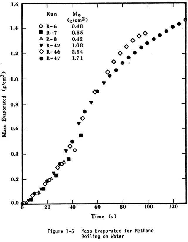
The mass of methane evaporated as a function of time is shown in Figure 1-6. As can be seen, methane evaporated slowly at first but then the rate of evaporation increased and reached a peak after about 40 seconds (Figure 1-7). Ice patches began to form after a few seconds

(%5 s) and these grew radially, eventually covering the water surface (%20 s).

Ethane displayed initial boiling rates (and heat fluxes) higher than those for methane. As in the case of methane, the boiling rates increased with time reaching a peak after about 15 seconds. Subse-quently, the boiling rates decreased significantly. Ice formation took place at a faster rate than with methane.

Propane boiled very rapidly during the first few (-5) seconds. The boiling rates then dropped to considerably lower values. Highly

irregular ice was formed very quickly (<1 s).

Methane-ethane mixtures (0.80 5 xC : 0.985) displayed high

initial boiling rates. These rates increased with time reaching a peak within 10 to 25 seconds. A layer of ice covered the water surface in

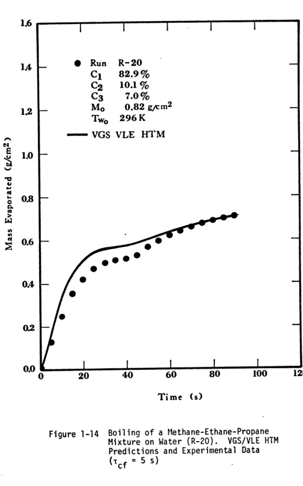
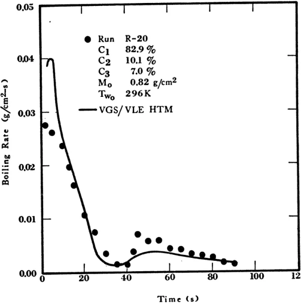
about 5 seconds. Extensive amounts of foam were generated. When methane-ethane-propane mixtures were spilled on water, rapid boiling took place in the first few seconds and was accompanied by extensive foam, 10 to 15 cm high. In most cases, the maximum boiling rate was achieved within the first 8 seconds; the boiling rates then decreased with time. In many tests secondary peaks in the boiling rates were observed; their magnitudes were, however, much lower than the initial peak. These effects can be seen in Figures 1-8 and 1-9.

0 0 vO O 60 Time (s)

Figure 1-6 Mass Evaporated for Methane Boiling on Water I Run 1.6 1.4 1.2 0 Y R-6 R-7 R-8 R- 42 R- 46 R- 47 Mo (g/cm2 ) 0.48 0.55 0.42 1.08 2.54 1.71 O

O A

,p$

Time (s)

Boiling Rates for Methane E U ID 4. Lw C 0.03 0.02 0.01 0.00 Figure 1-7

Run R-20 Cl C₂ C₃ 82.9 % 10.1% 7.0% Mo 0.82 g/cm2 000000 0 0e* **Og 20 40 60 80 100 Time (s)

Figure 1-8 Mass Evaporated for Run R-20, Ternary Mixture 1.6 1.4 1.2 C,4 E V 4.d₀ '3 tt {q 1.0 0.8 0.6 0.4 0.2 0.0 120

Run R-20 Cl C₂ C3 82.9% 10.1% 7.0% Mo 0.82 g /cm 2 0

*

r

Figure 1-9 Boiling Rates for Run R-20, Ternary Mixture 0.05 0.04 F-0.03 0.02

0.01

The addition of small amounts of nitrogen to methane and to methane-ethane-propane mixtures did not affect their boiling rates significantly.

Dicussion oj Resuts

Upon initial contact with water, a surface at a temperature approximately 180 K above its boiling point, methane film boils. The

insulating behavior of the film results in the low initial heat fluxes observed. As energy is removed, the upper layers of water cool and ice forms. The temperature of the ice surface continues to decrease until the difference in temperature is no longer high enough to main-tain stable film boiling. Transitional boiling begins and the heat fluxes increase, reaching a peak when nucleate boiling (direct methane-ice contact) is fully established. Thereafter, the heat fluxes, and the boiling rates, decrease.

Initially, ethane transition boils on water. Nucleate boiling, and the peak boiling rate, is attained faster than with methane. Propane, with a saturation temperature only 42 K below the freezing point of water, nucleate boils upon initial contact. The heat flux, and boiling rates, are therefore highest at the initial contact time.

The evaporation of mixtures is a far more complicated situation. In addition to shifts in boiling regimes, one must consider the change in composition and saturation temperature of the residual liquid as preferential evaporation of the more volatile components takes place.

Consider a binary mixture of 90% methane and 10% ethane. The saturation temperature is close to that of methane. As in the case of pure methane, a vapor film is formed. As a vapor bubble is formed,

the liquid at the base of the bubble becomes depleted in methane since the vapor bubble is made up primarily of the most volatile component. The liquid remains essentiallyisathermal but a thin liquid layer at the base of the bubble has changed significantly in composition (heat

transmission and evaporation being much faster than diffusional mass transfer). This means that for this thin liquid layer to be in equi-libria the pressure must drop. Or in other words, the vapor pressure of this thin layer at the base of the bubble becomes less than one atmosphere. As some of the vapor in the film evaporates into the

growing vapor bubble, the low vapor pressure of this thin surface layer hinders the replenishment of the vapor film. Thus, the vapor film collapses. The bubble pinches off and carries in its wake the

ethane-rich layer which then mixes with the bulk of the liquid. Fresh liquid rushes in and a temporary liquid-liquid contact is made which allows for high heat fluxes. The vapor film is reformed and the cycle begins again. The direct contact causes the water and the ice, when formed, to cool more rapidly. Soon, the surface temperature of the ice drops enough that the difference in temperature with the boiling liquid is

no longer large enough to regenerate the film, and nucleate boiling is established. Thereafter, the heat fluxes and boiling rates begin to decrease.

In the case of mixtures richer in heavier hydrocarbons, the decrease in vapor pressure is even more dramatic, so the film around a bubble collapses more easily, and the peak flux can be attained at shorter times.

This theory presents a plausible mechanism to explain why there is an increase in initial boiling rates upon addition of heavier hydrocarbons to methane.

The eventual enrichment of the bulk liquid in heavier hydrocarbons due to the preferential evaporation of methane plays a very important role in the latter part of the boiling process. The saturation temper-ature of a mixture of methane and ethane, for instance, will not change appreciably until the residual methane is less than about 20%. The saturation temperature then quickly rises to the saturation temperature of ethane.

Consider again the 90% methane, 10% ethane mixture spilled on water; after the ice has formed it begins to cool and approach the saturation temperature of the mixture. The bulk of the liquid is

being depleted in methane and when nearly all the methane has evaporated, the saturation temperature of the cryogen begins to increase towards

that of pure ethane. Considering the situation from the ice point of view, its surface is placed in contact with a body at a very low

temperature. As the surface of the ice is approaching this low temper-ature, the temperature of the cold body begins to increase. Obviously, this upsets the temperature gradient near the interface resulting in very low heat fluxes.

Furthermore, the residual liquid must be warmed to the (continuously increasing) saturation temperature. Thus, most of the modest amount of energy being transferred goes into heating the residual mixture and very little into actual evaporation. The overall result is a very low rate of evaporation.

A similar situation develops with methane-ethane-propane mixtures.

Once the methane is depleted, the mixture is primarily ethane and propane. A new plateau in saturation temperature is reached, and the heat flux

preferentially evaporates ethane, yielding a secondary, small peak in the boiling rate. The difference in volatility between ethane and propane is not as drastic. Thus, although the behavior upon exhaustion of ethane will be similar to the previous exhaustion of methane, it is not as pronounced; in fact, a third peak is not necessarily expected.

Heat Transfer Models

The first step in a scheme to predict the evaporation of LNG on water is to determine the amount of energy that is transferred across the water (ice)/LNG interface. This can be accomplished by solving the equations for transient conduction involving solidification

(Stefan's Problem). In the present case, the boundary condition at x = 0 (water/ice-LNG interface) must yield the temperature at that point. Since a vapor film is formed initially, the temperature at x = 0 will not reach the temperature of the cryogen until the film collapses.

Regaession of Swuface Temperature by Using Convolution Integral6

Pure methane was spilled on a solid block of ice and the following convolution integral was used to determine the ice surface temperature as a function of time:

e(0,T) =

f

0

which can be rewritten as follows

2rT

2

Oe(0,) =k q - ) du (1-15)

0

where e is the change in surface temperature from the initial ice temperature and k and a are the temperature-averaged thermal conduc-tivity and diffusivity of ice, respectively. The experimental values of heat flux (evaporation rate x heat of vaporization) were used in the integrand. The results are shown in Figure 1-10.

Similarly for methane spilled on water, the following convolution integral was used.

erf (KB/2/a ₁) -2/- 2

O(0,T) = kI q( - u2-) du (1-16)

0

where e is the departure of the surface temperature from the freezing point, kI and al are the temperature-averaged thermal conductivity and

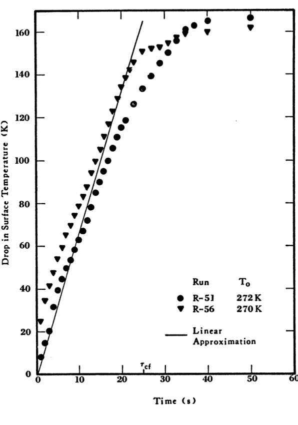
diffusivity, respectively, of ice. B is the ratio of the density of water to that of ice and K is a parameter which depends on the properties of ice, water, heat of fusion of ice, water and cryogen temperatures. Again the experimental heat fluxes, q, are used in the integrand. The results are shown in Figure 1-11.

As can be seen in these figures, the surface temperature drop can be approximated by a linear drop over a period of time Tcf, the time for the total collapse of the vapor film.

Time (s)

Figure 1-10 Drop in Surface Temperature of Ice after a Methane Spill

160 140 120 100 80 60 40 20

180 160 140 120 -a 100 - w 80 onn 0 60 Run T * R-42 288K V R-47 284K 20 - Linear Approximation 0 I 'cf " 0 10 20 30 40 50 Time (s)

Figure 1-11 Drop in Surface Temperature of Ice after a Spill of Methane on Water

Vatiable Grid Size Heat Trantr Model

In order to allow for the time-varying surface temperature con-dition, and for the variation in thermal properties of ice with

temperature, a numerical, variable grid size heat transfer model was developed. In such a model, the differential equations are replaced

by difference equations.

The substrate of thickness E is, at all times, divided into an ice layer of thickness e, and a water layer of thickness E - e. In turn, each layer is divided into m points. Consequently, the spacing between grid points in the ice layer will be AxS=e/m and in the water layer AXL = (E - e)/(M - m) where M is the total number of grid points equal to 2 m. As time progresses, the depth, e, of the freezing front

increases but the freezing front always corresponds to the m-th grid point.

The movement of the freezing front is given by

de _ 1 k m-2 - 4-1 + 3m + k m+2 - 4m+l + 3 m

d- pAHfus i 2(e/m) w 2(E - e)/(M - m) (-16)

The temperature at the n-th grid point in the ice layer is given by

de i - o k (e ) k (e

-den - n n+l n-l de 1 (n-l/2(n-1 n) - kn+1/2(en - en+l)

dT e 2 dr PnCp (e/m)2

n _(1-17)

de e - \ / + 2 + \ n M-n n+1 n-I de a n-1 + n n+ 1 + a (1-18) d E-e \ 2 d w (E-e)2/(N-m)2 Finally, e+ = eT + AT de/dT (1-19) and en,+AT = en, + AT dn/dT (1-20)

The properties of ice are allowed to vary with temperature, whereas those of water were taken as constants since they vary little

in the range of interest.

Making use of the results obtained with the convolution integral, the temperature at the surface is allowed to approach the cryogen temperature linearly over a period of time T_cf'

The model as described thus far, can be used only with pure components. For mixtures it must be coupled with the VLE model

previously described. The VLE model provides the Variable Grid Size (VGS) model with the cryogen temperature. The VGS model computes the total heat flux across the substrate/cryogen interface. After sub-tracting the heat required to raise the temperature to the new satur-ation temperature, the mass evaporated is determined. This evaporsatur-ation

is fed to the VLE model which then determines the new residual liquid composition and saturation temperature. The cycle is then repeated.

The results obtained with the VGS/VLE HTM for a binary methane-ethane mixture and for an LNG mixture are shown in Figures 1-12

Time (s)

Figure 1-12 Boiling of a Methane-Ethane Mixture on Water (R-1). VGS/VLE HTM Predictions and Experimental Data (Tcf = 25 s)

cf 1.6 1.4 1.2 cc 0 0. U u IA 1.1 0.8 0.6 0.4 0.2 0.0

* Run R-I C1 98.5% C2 1.5% Mo 0.80 g/cm2 Two 295 K - VGS/VLE HTM 0.01

/

Figure 1-13 Evaporation Rates of a Methane-Ethane Mixture on Water (R-1). VGS/VLE HTM Predictions and Experimental Data (Tcf = 25 s)

0.03

0.02

--Time (s)

Figure 1-14 Boiling of a Methane-Ethane-Propane Mixture on Water (R-20). VGS/VLE HTM Predictions and Experimental Data

(Tc = 5 s) 1.6 1.4 1.2 1.0 0.8 0.6 0.4 E I 4.' 0 0.'U U2 0.0 ₁₂₀

0.05 0 Run R-20 C1 82.9 % 0.04 _{C2 10.1 %} C3 7.0 % Mo 0.82 g/cm2 .4 Two 296K " 0.03 - VGS/ VLE HTM 0.01 0 20 40 60 8 100 Time (s)

Figure 1-15 Evaporation Rates of a Methane-Ethane-Propane Mixture on Water (R-20).

VGS/VLE HTM Predictions and Experimental Data (Tcf = 5 s)

through 1-15. The VGS/VLE HTM predictions agree well with the experi-mental data; thus reinforcing the qualitative explanations previously given.

The only variable parameter in the model, 'cf the time for the collapse of the vapor film, has been correlated as follows

Scf= 45 x - 40 x0. 2_{- 10 x0.1 (s)}

cf 1 C₂ C₃

where x's are mole fractions. The following restrictions are made:

Tcf > 0, and it should only be used within the LNG compositional range (x2C 0.20, x C 0.10).

2 3

Thus, the VGS/VLE HTM model becomes the first successful scheme to predict a priori, the evaporation of confined spills of LNG on water.

Conclusions

The following conclusions are made regarding the evaporation of confined spills of liquefied natural gas (LNG) on water.

* Methane film boils on water until the ice layer which forms cools sufficiently to promote nucleate boiling. The heat fluxes, and

boiling rates, increase with time until nucleate boiling is achieved, thereafter they decrease.

* LNG mixtures undergo a preferential evaporation of the more volatile components. This evaporation causes a rise in the saturation temper-ature of the residual liquid. The composition of the vapor and the

residual liquid, as well as the saturation temperature, can be deter-mined from vapor-liquid equilibria and mass balance considerations. * LNG mixtures film boil on water upon initial contact. The

prefer-ential evaporation of methane causes a drop in the vapor pressure of the liquid at the base of the bubbles being formed; such a pressure drop results in the collapse of the vapor film around the bubble. * The higher the heavier hydrocarbons content in the LNG mixture, the

faster the vapor film collapses and the sooner nucleate boiling is established.

* As methane is exhausted, the saturation temperature increases, causing a decrease in the heat flux across the ice/LNG interface. Furthermore, most of the energy transferred at this time goes into warming up the cryogen to the rising saturation temperature.

* The decrease in the surface temperature of the substrate, approaching the cryogen temperature, may be approximated by a linear drop over a period of time Tcf* This period of time Tcf is a function of the chemical composition of the cryogen.

* Based on the above considerations, a heat transfer model that draws information from the vapor liquid equilibria model has been developed. This model predicts successfully the evaporation of confined spills of LNG on water.

Now that the effect of composition on the boiling of LNG on water is understood, research efforts can be directed towards the determination of the effect of spreading and wave motion on the boiling of LNG in an open sea spill.

II. PREVIOUS WORK RELEVANT TO THE BOILING OF LNG ON WATER Regimes of Boiling

When a liquid at its saturation temperature contacts a hot surface at a temperature above that of the liquid, a phase transformation from

liquid to vapor, i.e. boiling, takes place. This phenomenon is known as saturated or bulk boiling as opposed to subcooled or local boiling in which the bulk of the liquid is below the saturation temperature.

If the temperature of the hot surface is only slightly above the saturation temperature of the liquid, heat transfer takes place by convection and evaporation occurs at the free surface of the liquid.

Increasing the hot surface temperature causes the liquid near the hot surface to superheat slightly; bubbles form at the hot surface and rise

through the liquid. This form of boiling is called nucleate boiling. In this regime the boiling liquid is in direct contact with the hot surface, and its boundary layer is intensely disturbed by the vapor bubbles. Furthermore, as the bubbles detach and begin to rise, they drag some superheated liquid from the layer adjacent to the hot surface

into the core of the rising stream, creating an intensive macroscopic transport of heat from the hot surface into the bulk of the boiling liquid. Thus, essentially all the heat is transferred directly to the liquid which divests itself of the energy by evaporation into the vapor (Kutateladze, 1963). The bubbles in this regime are formed at

certain favored spots on the surface, the so called active site. or cavitie4; some gas or vapor is present in these active sites. Upon heating, the vapor pocket grows by evaporation at the liquid-vapor

interface near the heated wall. As a bubble pinches off and detaches from the surface, some vapor is trapped in the cavity. This vapor initiates the generation of a new bubble (Rohsenow and Choi, 1961).

For a spherical bubble of radius R, the liquid and vapor pressures are related by equilibrium thermodynamics.

2a Pvap - Pliq = R

Using the Clausius-Clapeyron equation, it can be shown that the vapor temperature for such a bubble is

= Tsat + 2 AVvap

v

sat

(

R AHvap

A minimum degree of superheat is then required for the generation of bubbles in a given cavity. As the temperature of the heating surface is increased, more and smaller nucleation sites are activated, thus increasing the rate of bubble production. This increase in bubble generation as well as the macroscopic agitation near the hot surface are responsible for the high heat fluxes observed in this regime. The increase in heat flux does not continue indefinitely. As the bubbles depart dragging some superheated liquid, a mass of cold liquid must flow from the bulk to the hot surface. When bubble generation is large enough that their rise interferes with the flow of the replenishing liquid, a blanket of vapor essentially covers the hot surface. In most boiling studies an electrically heated filament is used as the

transfer to the liquid and the filament temperature increases from point

a towards point c in the boiling curve shown in Figure 2-1. Generally the temperature at point c is higher than the melting point of most metals and the wire melts before reaching this point. Thereafter,

point a is called the burnout point or peak nucleate flux (Rohsenow and Choi, 1961).

Increasing the temperature of the heating surface past point b results in a stable vapor blanket; this is the film boiling regime. Heat must be transferred through the vapor film and the vapor bubbles are formed at the vapor film-boiling liquid interface. The low thermal conductivity of the vapor is responsible for the low heat transfer rates observed in the film boiling regime. The lowest temperature capable of sustaining a stable film is called the Leidenfrost point.

Between the nucleate burnout and the Leidenfrost points lies the transition regime, in which the vapor film collapses intermittently. The random nature of the collapse of the film makes this regime extremely hard to characterize.

Effect of Surface Roughness on Pool Boiling

The degree of smoothness of the heating surface affects the boiling characteristics in the nucleate regime. There is both a change in position as well as slope of the nucleate boiling curve. As shown in Figure 2-2, the nucleate regime expands to higher temper-ature differences for smoother surfaces and the transition regime shrinks. But, the film boiling regime remains essentially unaffected.

1000 1

Convective Nucleate Transition Fi Im

I I Peak Nucleate SFlux E -Y 100 -10 _II b ! Leidenfrost Point I I 1 10 100 1000 10000

AT, Thot surface "Tsaturation (K )

NIIII - Nucleate ma I Transition * Transition . I I I 1 l1 Fi Im Nucleate -Burnout

/

,,,,I

I I I I 11

1000 (K)

Figure 2-2 Effect of Surface Conditions on Boiling Heat Transfer

1000 Surface Surface 100 10 Leidenfrost Point i I I I a a I I I . . . n

__