Perception for Robotics: Part II

HAL Id: cel-02129241

https://hal.inria.fr/cel-02129241

Submitted on 14 May 2019

HAL is a multi-disciplinary open access

archive for the deposit and dissemination of

sci-entific research documents, whether they are

pub-lished or not. The documents may come from

teaching and research institutions in France or

abroad, or from public or private research centers.

L’archive ouverte pluridisciplinaire HAL, est

destinée au dépôt et à la diffusion de documents

scientifiques de niveau recherche, publiés ou non,

émanant des établissements d’enseignement et de

recherche français ou étrangers, des laboratoires

publics ou privés.

Distributed under a Creative Commons Attribution - NonCommercial| 4.0 International

Perception for Robotics: Part II

Cédric Demonceaux

To cite this version:

Cédric Demonceaux. Perception for Robotics: Part II. Doctoral. GdR Robotics Winter School:

Robotica Principia, Centre de recherche Inria Sophia Antipolis – Méditérranée, France. 2019.

�cel-02129241�

AUTHOR:

Cédric Demonceaux1

1_{ImViA - VIBOT ERL CNRS 6000, Université Bourgogne Franche-Comté}

P

ERCEPTION FOR

R

OBOTICS

: P

ART

II

Some words to introduce the chapter contents:

«What is around me?»knowing how to answer to this question is essential for a robot to navigate safely in its environment. In this part, we will try to find some answers by introducing some tools for helping the robot to perceive the world. Thus, we will present different sensors (lasers, radars, cameras, RGBD sensors) which allow to build a 3D map of the scene where the robot is navigating. Then, we will mainly focus on cameras since these sensors give a rich information about the scene. We will see how we can extract features from the image in order to provide a 3D perception of the world. This chapter presents the main concepts required to start computer vision applied to robotics. It is not an exhaustive study, thus we can only strongly recommend to read the articles and books cited to deepen the knowledge .

Table 2: Specific notations used in this chapter

K , Calibration Matrix

P , Projection Matrix

C , Camera center

X = (Xm_{, Y}m_{, Z}m_{) , 3D point in framem}

x = (u, v) , pixel

Eij , Essential matrix between imageito imagej

X , 3D point cloud

T = (R, t) , Rigid transformation with a rotationRand translationt.

A

CTIVE AND PASSIVE SENSORS

An active sensor uses external projecting devices that emit light wavelength, signal or patterns to interact with the scene. The data generated by this external source are gathered by the sensor to deduce information on the environment around the robot. This conversion can be carried out in many ways depending upon the type of sensors. Based on their working principles, there are mainly 3 types of active sensors used in robotics : Lidar, Structured-Light and time-of-flight. On the opposite, passive sensors gather target data through the detection of vibrations, light, radiation, heat or other phenomena occurring in the environment without external devices. Commonly, the passive sensors used in robotics are cameras/image sensors. In the following, let us describe in few lines the different characteristics of these sensors.

L

I

DAR

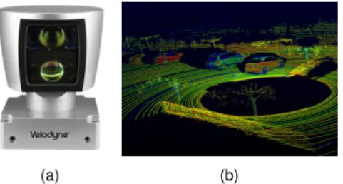
The LiDAR instrument emits rapid laser signals which bounce back from the obstacles. The sensor positioned on the instrument measures the amount of time it takes for each pulse to bounce back. Thus, the instrument can calculate the distance between itself and the obstacle with accuracy. It can also detect the exact size of the object. LiDAR is commonly used to make high-resolution maps (Fig. 1).

(a) (b)

Figure 1: LiDAR sensor (Velodyne) and raw data.

R

ADAR

The RADAR system works in much the same way as the LiDAR, with the only difference being that it uses radio waves instead of laser. In the RADAR instrument, the antenna doubles up as a radar receiver as well as a transmitter. However, radio waves have less absorption compared to the light waves when contacting objects. Thus, they can work over a relatively long distance. The most well-known use of RADAR technology is for military purposes. Airplanes and battleships are often equipped with RADAR to measure altitude and detect other transport devices and objects in the vicinity.

S

TRUCTURED

-

LIGHT

Structured-light based sensors project bi-dimensional patterns to estimate the dense depth information of the object surface points. Depending upon the application, the projected patterns can be a single or multiple frames. The main role of the projected patterns is to establish correspondences between the known pattern and camera measurements in a relatively easy manner. Note that the measurements vary according to the 3D model of the object. This variation encodes the scene depth information, which can be recovered using a triangulation tool similar to the one developed in next section for a pair of 2D cameras. Nowadays, these type of sensors are often used in robotics for many applications (localisation, 3D reconstruction, gesture recognition...) because they are light, small, low energy consuming and allow to obtain color and 3D information very quickly at each shot (Fig 2a). Nevertheless, they are really sensitive to the light conditions this is why these sensors are used for indoor application. For outdoor application, we will rather used time-of-light sensors.

T

IME

-

OF

-

FLIGHT

Time-of-flight cameras consist of emitter and receiver units (Fig 2b). The emitter unit generates a laser pulse that impinges on the targeted object surface. The reflected laser pulse is then detected by the receiver unit along with the roundtrip travel time from transmitter to the receiver. This round-trip travel time provides the 3D position of the object surface point using the speed of light and the ray projection angle. Time-of-flight cameras in principle perform point-to-point reconstruction. These cameras can cover large distances and also provide accurate depth estimation though the coverage is limited by the allowed laser power. Additionally, time-of-flight cameras are rather costly and face scanning difficulties with surfaces exhibiting certain reflective, gloss or color properties. To improve the sensitivity and accuracy, both amplitude and frequency modulated strategies have been adopted for close range distance measurements. Other active sensing technologies include interferometry, laser triangulation, Moiré fringe range contours, etc. A detailed study about existing active as well passive sensors can be found in [31].

(a) Structured-light sensor: Kinect V (b) Time-of-flight: KinectV2

(c) 3D cloud of point acquired by KinectV1 (d) 3D cloud of point acquired by KinectV2

Figure 2: Structured-light and Time-of-flight sensors ([39])

I

MAGE SENSORS

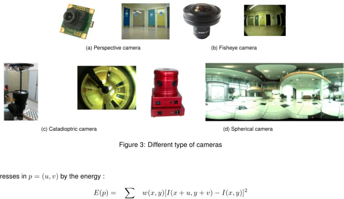
Image sensors use the ambient light source and convert it into a 2D image. 2D cameras allow capturing high-quality details (due to a combined technological progress in both optics and CCD or CMOS sensors) but require external tools and information to recover the 3D scene. Most common methods, namely stereo vision and monocular or multiple-view structure from motion, recover depth information from two or multiple such projections using the concept of image parallax. In the case of a stereo camera pair, the image parallax is generated due to their positioning. However, monocular cameras must go under motion to generate the parallax. This approach is referred to as Structure-from-Motion (SfM). In recent days, the SfM-based techniques are very popular because they offer a simple, inexpensive, and accurate solution. Additionally, it allows us to reconstruct large scenes by moving the cameras covering the whole scene or using acquisitions from many cameras [1]. Nowadays, these cameras are very popular and widespread as they are affordable and reliable. It exists varieties of optics models for 2D cameras, the choice of the optics strongly depend of the application (Fig 3). For example, large field of view (panoramic, fisheye) even spherical field of view can be really useful in robotics, because they allow to have a maximum of information with only one shot.

In the following sections, we will try to answer to these questions: how to extract information in the image? How to modelize the image formation? How to localize 2D cameras in the scene and how to recover the 3D? Finally, we will focus on 3D sensors.

2D

CAMERAS

:

SOME BASIC IMAGE PROCESSING TOOLS

F

EATURES EXTRACTION

To compare two images, it requires to find corresponding features across them. This problem has been studied since the 80s [24]. Most methods are based on two steps : feature detection where we identify the points or areas of interest in the images and feature description which represents the feature as a descriptor. These descriptors correspond to a signature which allow to determine correspondence between the views. A lot of methods have been developed, we will described the main ones below.

HARRIS

The idea behind the Harris method [15] is to detect points based on the intensity variation in a local neighborhood: a small regionW around the feature should show a large intensity change when compared with windows shifted in any direction. It

(a) Perspective camera (b) Fisheye camera

(c) Catadioptric camera (d) Spherical camera

Figure 3: Different type of cameras

expresses inp = (u, v)by the energy :

E(p) = X

(x,y)2W

w(x, y)[I(x + u, y + v) I(x, y)]2 (1) wherew(x, y)is weighted function (simplest casew = 1). For nearly constant patches, thisE(p)will be near 0 whereas for very distinctive patches,Ewill be larger.

By a Taylor expansion,Eis approximated by :

E(p)_{' [u, v]M[u, v]}T (2) where the matrixM corresponds to the image derivatives :

M = X (x,y)2W w(x, y)  I2 x IxIy IxIy Iy2 (3) This matrix plays an important role to characterize the homogeneity of a patchW aroundpthanks to the disparity ofx

andyderivatives. This disparity can be estimated by the eigenvalue 1and 2ofM. Thus, Harris proposed the corner

response measurement which is large for a corner :

R = det(M ) k(traceM )2 (4) wherekis an empirically determined constant (2 [0.04, 0.06]). This method is really efficient, invariant to image rotation but not scale invariant. In this way, Lowe [21] has proposed an improvement using a multiresolution scheme.

SIFT

SIFT detector [21] (Scale-Invariant Feature Transform) consists of four major stages: (1) Scale space extreme detection; (2) keypoint localization; (3) orientation assignment; (4) keypoint descriptor. In the first stage, a multiresoltuion scheme is performed in order to determine potential interest points that are invariant to scale and orientation. These are the local scale-space maxima of the Difference of Gaussian (DoG) which is obtained by subtracting the different Gaussian scales:

D(x, y, ) = (G(x, y, k ) G(x, y, ))⇤ I(x, y) (5) whereG(x, y, )is a Gaussian blur at scale . The points with low contrast are rejected based on the same idea under the Harris method where theM matrix. To obtain descriptors that invariant to rotations, an orientation histogram was formed from the gradient orientations of each local maximum of the DoG function within a region around the keypoint. The final stage of SIFT constructs a descriptor by considering the direction of a keypoint which is gradient strength is maximal.

Typically, an adjacent 16x16 region is determined by put the keypoint in the center. After the region is chosen, SIFT divides this region into4_{⇥ 4}sub-regions with 8 orientation bins in each. Since there are 4 x 4 = 16 histograms each with 8 bins the vector has 128 elements. Thus, the meaningful descriptors are extracted from the image that are compact, highly distinctive and yet robust to change in illumination and camera viewpoint.

SURF

SIFT are robust but really time consuming. To overcome this problem and inspired by the SIFT descriptor, Bay has proposed the SURF detector [5] (Speeded Up Robust Features). It is able to generate scale and rotation invariant interest points and descriptors. Compared to SIFT, SURF uses 2-D Haar wavelets which are an approximation of DoG but more efficient to compute thanks to integral images. For keypoint detection, it uses the sum of the 2D Haar wavelet response around the point of interest. A 2D Haar wavelet is obtained by an integer approximation to the determinant ofM matrix that extracts blob-like structures at locations where the determinant is maximum. Therefore, the performance of SURF can be attributed to non-maximal-suppression of the determinantsM matrices. In description phase, firstly the neighborhood region of each keypoint is divided into a number of 4x4 sub-square regions. Then, it computes the response of a 2D Haar wavelet response each sub-region. Again, this procedure can be computed with aid of the integral image. Each response contributes four values to a descriptor, so each keypoint is described with a 64-dimensional (4x4x4) feature description of all sub-regions. Although the SURF method runs faster than the SIFT, but in some situations like viewpoint and intensity change it does not give good results as SIFT produced.

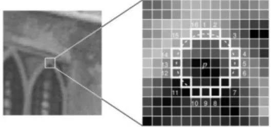
FAST

FAST corner detector [29] (Features from Accelerated Segment Test) is a corner detector that uses a circle of 16 pixels to classify whether a pixelpof intensityIpis actually a corner or not. Each pixel in the circle is labeled from integer number

1 to 16 as clockwise (Fig 4). If a set of N contiguous pixels in the circle are all brighter than theIpplus a threshold value

tor all darker than the intensity of candidate pixelpminus threshold valuet, thenpis classified as corner. To make the algorithm fast, first compare the intensity of pixels 1, 5, 9 and 13 of the circle withIp. If at least three of these four pixels

satisfies the threshold criterion so that p is chosen as an interest point. On the other hand, if at least three of the four pixel values (I1,I5,I9andI13) are not above or belowIP + t, then p is not an interest point (corner). Else if at least three of

the pixels are above or belowIp+ t, then check for all 16 pixels and in this case 12 contiguous pixels should fall in given

criterion. Likewise, repeat the procedure for the all others remaining pixels in the image. Because of the some limitations such as for N<12 the algorithm does not work well, the choice of pixels is not optimal and multiple features are detected adjacent to one another, a machine learning approach has been employed to the algorithm to deal with these issues.

Figure 4: Fast corner detector

BRISK

Although the local features obtained by vector-based descriptors such as SURF, SIFT give successful results in terms of an image representation, using the descriptors of them is not an efficient way. To address this challenge, several binary descriptors computed directly on image patches and BRISK [20] (Binariy Robust Invariant Scalable Keypoints) is one of them. BRISK is based on FAST detector and consists of three parts: a sampling pattern, orientation compensation and sampling pairs. In here, taking a sampling pattern around the keypoint refers to points spread on a set of concentric circles, which are used to determine a point is whether a corner or not in FAST detector. Then these pairs are separated two subsets, short-distance pairs and long-distance pairs. To achieve rotation invariance, the direction of each keypoint is determined by taking the sum of computed local gradient between long-distance pairs and short-distance pairs are

rotated based on obtained orientations. Finally for all the pairs, the intensity values of the first and second points in the pair are compared, i.e., if the value of first point is larger than the second then output is 1, else 0. Hence, after going all 512 pairs, leading to a descriptor with 512 bits in length. In matching case, the Hamming distance is used instead of Euclidean distance due to its short execution time.

ORB

ORB detector [30] (Oriented FAST rotated BRISK) is a combination of FAST and BRIEF. To extract keypoints, it modifies the FAST detector as scale invariant by constructing a scale pyramid of the image. At each scale, keypoints are detected by illustrating the FAST detector. Once the keypoints detected, the Harris corner measure is employed to sort them and only top N points are chosen based on a threshold. To obtain rotation invariant features, first-order moments is used to compute the local orientation through an intensity centroid which refers to the weighted averaging of pixel magnitudes in the local patch. This method is nowadays the most efficient approach and is used in many SLAM approaches as ORB-SLAM [26].

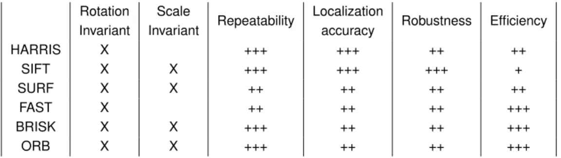
The table 3 summarizes the properties and performance of these feature detectors. For an exhaustive review, we warmly recommend to read [37]. Rotation Invariant Scale Invariant Repeatability Localization

accuracy Robustness Efficiency

HARRIS X +++ +++ ++ ++ SIFT X X +++ +++ +++ + SURF X X ++ ++ ++ ++ FAST X ++ ++ ++ +++ BRISK X X +++ ++ ++ +++ ORB X X +++ ++ ++ +++

Table 3: Comparison of some feature detectors

O

PTICAL FLOW

Instead of finding feature points in the each images, some methods propose to estimate the motion in the video sequence when two consecutive images have been taken in a short time with few modifications. This motion, called optical flow, [11] is really useful in many application: obstacle avoidance [40], action recognition [34], video segmentation [36]...

Let us consider an image sequenceI((x(t), y(t)), t), the optical flow methods compute the motion between two con-secutive frames which have been taken at timestandt + 1at every pixel position by estimating the apparent motion

!_{v ((x(t), y(t), t) = (}dx dt(t),

dy

dt(t)). If we suppose the brightness constancy constraint which means that the luminosity

does not change along the time :

I((x(t), y(t)), t) = I((x(t0), y(t0)), t0) 8t. (6)

This can be rewritten:

dI dt((x(t), y(t)), t) @I @x dx dt((x, y), t) + @I @y dy dt((x, y), t) + @I @t((x, y), t) = 0 (7) Thus, !

rI((x, y), t).!v ((x, y), t) +@I

@t((x, y), t) = 0, (8)

where!_{rI = (}@I @x,

@I

@y) = (Ix, Iy). This linear equation is not sufficient to compute!v (two unknowns, one equation) and

we have to add another constraint. The optical flow methods differ according to this constraint. Two main approaches exit : dense technics which expect smoothness of the flow field and sparse technics which suppose a constant optical flow in the neighborhood.

DENSE TECHNICS

- H

-S

The fundamental principles of optical flow estimation by variational (dense) methods were proposed by Horn and Schunck in 1981 [16]. The idea is to define a functional composed of two terms. The first term is based on the assumption of brightness constancy constraint and is defined as follows

H1(!v ) = Z Z ✓ ! rI.!v + @I @t ◆2 dxdy. (9)

The second term, called regularization term, penalizes first-order variations in the vector field!v H2(!v ) =

Z Z

k!rvk2dxdy. (10) Thus, Horn and Schunck estimate!v which minimizes:

E(!v ) = H1(!v ) + ↵2H2(!v ) (11)

where↵is a penalization term. The main drawbacks of this method is the introduction of the Tikhonov term (H2) which

induces a strong penalization of gradients. This strong penalization leads to excessive smoothing of the optical flow. Therefore, it is not possible to find the spatial discontinuities of the optical flow.

Since, different authors have proposed other terms for regularization to preserve discontinuities in the flow by introducing so-called "robust" penalization term (M-estimator).

S

- L

K

Lucas and Kanade [22] were the first to propose a sparse method. To do this, they minimize an energy composed only of the brightness constancy constraint. To overcome the aperture problem, they assume the flow!v constant on a small neighborhood of the point(x, y). This functional is defined as follows:

E(!v (p, q)) = min!_v X (p,q)2W(p,q) w2(p, q)  ! rI(p, q).!v (p, q) +@I @t(p, q) 2 (12) whereW(p,q)is a neighborhood of(x, y)andw(x, y)a gaussian. The solution is computed by:

!_{v (p, q) = M} 1 "P (p,q)2W(p,q)w(x, y)IxIt P (p,q)2W(p,q)w(x, y)IxIt # (13) whereM is the same image derivatives matrix defined in (3). This approach is really easy to implement and fast but the optical flow is computed if and only if the neighborhood is well textured (M is well-conditioned) which leads to sparse estimation. Nevertheless, this method continues to be widely used in robotics [3].

At this step, we are able to match points between several images or follow them on a video sequence. The study of the position of these points in 2D images can allow us to deduce the motion of the camera or the 3D structure of the scene. This is the subject of the following section.

2D

CAMERAS

:

FROM

2D

TO

3D

C

AMERA MODELING

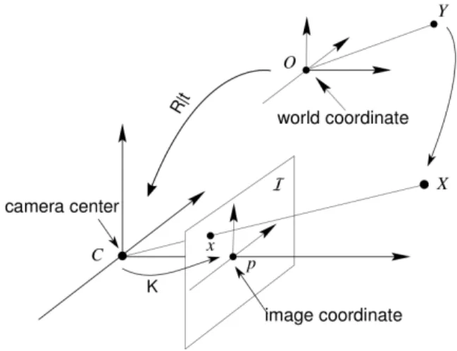
To compute 3D structure of a scene using 2D cameras, we need a model that describes how a camera projects the 3D world onto a 2D image. The most used model in computer vision is the pinhole model, which represents a perspective projection from 3D to 2D. This model is a good compromise between simplicity and true image formation of the most cameras used in robotics : perspective cameras, fisheye cameras, some catadioptric cameras, spherical cameras...

Figure 5: Image modeling

P

The pinhole model can be described by an optical centerCand an image planeI(Fig5). A 3D pointX = (Xc_{, Y}c_{, Z}c₎

in camera frame is projected on the image planeIinx = (u, v)as the intersection of the 3D light of sightXCwithI. To express in pixel coordinate, this projection is described with the intrinsic camera matrix K including :f the focal length (distance between_IandC,(u0, v0)principal point,mxandmyare the scale factors relating pixels to distance, is the

skew coefficient between thexand they) :

K = 2 4 ↵x u0 0 ↵y v0 0 0 1 3 5 (14)

In order to take into account the displacements of the camera, we choose a static coordinate system called world frame. Let us poseY = (Xw_{, Y}w_{, Z}w_{)the coordinates of the 3D pointQin the world frame. The position of the camera in this}

world coordinate frame is defined by a 3-space rotation matrixRand a translation vectortand the full camera model is given in homogeneous system as :

2 4 u v 1 3 5 ⇠ KR [I| t] 2 6 6 4 Xw Yw Zw 1 3 7 7 5 ⇠ P 2 6 6 4 Xw Yw Zw 1 3 7 7 5 (15)

The3⇥ 4matrixPis called projection matrix and maps 3D points to 2D image points. The termsKandR [I| t]are referred to as, respectively, the intrinsic and the extrinsic parameters of the camera. In robotics, this matrixP is crucial for visual odometry or 3D reconstruction application and requires calibration step to be estimated.

C

ALIBRATION

Calibrating a camera means computing theP matrix. To achieve this, most methods take several images at different position and orientation of a known planar checkerboard-like pattern (Fig. 6). The intrinsic and extrinsic parameters are then estimated through an over determined system solved a least-square minimization method. Many camera calibration exist, among these, the most popular one is given in [8].

E

PIPOLAR

G

EOMETRY

Given point correspondences between at least two 2D cameras and their intrinsic parameters, it is possible to recover both the motion between cameras and the scene structure. This concept is described in Figure 7 between two views. Letx1

andx2be corresponding image feature points given in camera coordinate frames attached toC1andC2respectively.

Figure 6: Camera Calibration: Image acquisition and results ([8]) .

Figure 7: Epipolar Geometry

The two-view imaging model is based on the fact that, given a point in one image, its corresponding point in another image must lie in a one-dimensional space known as epipolar line. Every epipolar line intersects in the epipole as shown in Figure 7 , wherex2(the point corresponding tox1) lies on the epipolar linel2that also passes through the epipolee2. This

happens because the camera centers, epipoles, image points, together with the observed 3D pointX, lie on the same plane such that back-projected rays from image points intersect in 3-space. Since the linel2must containe2andx2,l2

must also lie on the epipolar plane defined byC1,C2, andX. It is straightforward to express the normal vector of the

epipolar plane as[t21]⇥R21x1where the symbol[.]⇥denotes a skew-symmetric. Thus, we obtain the so-called epipolar

relationship between the corresponding pointsx1andx2as follows :

xT2[t21]⇥R21x1= xT2E21x1 (16)

The matrixE21is also known as the Essential matrix. By construction, the Essential matrix is of rank 2. In other words, the

essential matrix has five degrees of freedom: three from the rotation matrix and two from the translation vector. Therefore, it can be estimated from at least five point correspondences, as every pair of correspondences provides one equation of the form of (16). Then, the rotation and translation can be recovered by direct decomposition of the Essential matrix. The reader may refer [27] for more information on its estimation. The entries ofE21can be estimated only up to an unknown

scale factor. This eventually prohibits us from recovering the scale of the translation and the exact scale associated with the translation vector can never be known unless extra information are fed into the problem. In this context, the extra information of scale is always necessary for its unique recovery. Therefore, the translation vector is usually computed with a unit norm hence losing the true scale of the scene.

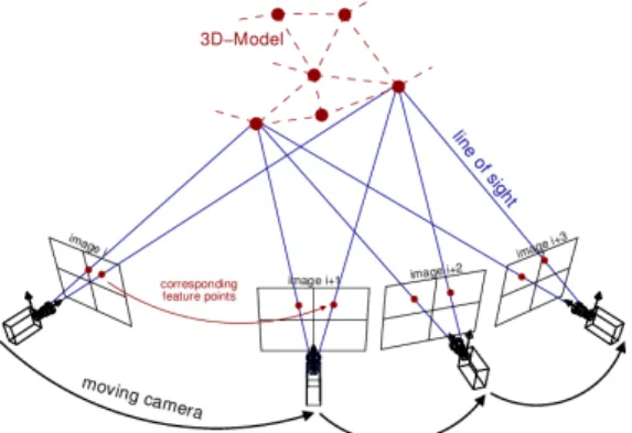
B

UNDLE ADJUSTMENT

The previous technic can easily recovered the rigid transformation between two views and thanks to a triangulation, we can also determine the depth (3D) on every points. When we deal with multiple view images, these 3D points are viewed in different positions. In this case, we use a bundle adjustment where we conjointly refine the 3D coordinates describing the scene geometry and the camera(s) position. Thus, assume thatn3D pointsXiare seen inmcameras

Figure 8: Bundle adjustment (Courtesy of http://www.theia-sfm.org/sfm.html)

with intrinsic parametersKjand letxijbe the projection of theithpoint on imagej. Letvij denote the binary variables

that equal1if pointiis visible in imagejand0otherwise and assume also that each camerajis parameterized by a rigid transformationTj = (Rj, tj). Bundle adjustment minimizes the total reprojection error with respect to all 3D point and

camera parameters, specifically

min (Rj,tj) n X i=1 m X j=1 vijd(KjRj[I| tj] Xi, xij)2, (17)

whered(x, y)denotes the Euclidean distance between the image points represented by vectorsxandy. Thus, Bundle adjustment [35] minimizes the reprojection error between the image locations of observed and predicted image points (Fig 8), which is expressed as the sum of squares of a large number of nonlinear, real-valued functions. Thus, the minimization is achieved using nonlinear least-squares algorithms such as Levenberg Marquardt [25] which has proven to be one of the most successful due to its ease of implementation.

3D

SENSORS

: 3D - 3D

In this part we suppose that we can obtain 3D data directly from the sensor (LiDAR or RGB-D cameras : Structured light, Time-of-light, Stereocamera...). These sensors have emerged as one of the most effective sensors to make robots autonomous because they become less and less expensive (LiDAR) and can give us photometric information RGB-D (color image plus depth) cameras. Thus, we consider two cases depending of the availability of the photometric information. Firstly, we will suppose that the sensor provides only 3D cloud of points at two consecutive times respectively

X = {X1, . . . , Xm}andY = {Y1, . . . , Yn}. Here, the goal is to find the rigid transformationRandtwhich minimizes

an error function by registering_Xand_Y. Many methods have been developed to solve this problem and the most popular algorithm is called Iterated Closest point (ICP). In the second case, if the 3D sensor also provides RGB some methods including RGB+depth have been developed by using conjointly 2D image constraint and 3D registration.

ICP

The ICP algorithm was presented in the early 90s for registration of 3D range data to CAD models [6]. The key problem can be reduced to find the best transformation that minimizes the distance between two point clouds. In robotics, ICP is really useful because the transformationRandtthat minimizes the error between two consecutive 3D acquisition is proportional to the motion of the robot. If the points ofX andYare matched, the problem consists in findingRandt

solution of : _n

X

i=1

kRXi+ t Yik2 (18)

The solution is computed by the SVD decomposition of the matrixW = U DVT ₌ Pn

i=1X0i⇤ Y0Ti whereX0 =

{X1 X , . . . , X¯ m X }¯ (resp.Y0) are the centered data and we have :

R = U VT (19)

In the general case, whenX andYare not matched, it’s not an easy problem and it’s solved iteratively by the following algorithm :

Algorithm 1 Compute the rigid transformationRandtbetween two point clouds_X and_Y input : two point cloudsX andY, an initialization (R0,t0),dmaxthreshold.

output : the rigid transformationRandt (R, t) _(R0, t0)

while not converged do fori 1to n do mi F indClosestP ointInY (RXi+ T ) if_kRXi+ T Yik 6 dmaxthen !i 1 else !i 0 end if end for

(R, T ) _{arg min}Pn_i=1!ikRXi+ T Yik2

end while

It exists many variations of this algorithm depending of outliers rejection, error measurement... a recent review can be read in [28]. Let us note that the ICP algorithm can be used to stitch consecutive 3D point clouds together. Moreover, with RGB information, it is possible to build the 3D scene with color information. In this case, RGB images can be used to match the 3D points by projective data association but also to detect a loop closure in order to reduce the inherent drift errors that we propagate by making consecutive maps created by ICP [17], [14].

D

ENSE

RGB-D

REGISTRATION

When we deal with RGB-D cameras, we can conjointly take into account 2D color information (RGB) and depth data (D). Thus, some authors propose to compute the 3D rigid transformationT = (R, t)by minimizing an error that includes photometric :

eI(p, X, t) = I(!(p,X , T ), t) I(p, t 1) (21)

where!(p,_{X , T )}is a warping function which back projects a 3D point_X with transformationT onI. and depth errors :

eD(p, X, t) = D(!(p,X , T ), t) D(p, t 1) (22)

whereD(p, t)is the depth of pixelpin image at timet. We can note that, (21) is a classical optical flow constraint equation (OFCE) term and (22) is equivalent to a flow point-to-plane ICP. The classic dense RGB-D registration consists of using jointly (21) and (22) as b T = arg min T X p ⇢I(eI(p, X, t)) + ⇢D(eD(p, X, t)) (23)

With⇢are robust M-estimators to reduce the effects of self occlusions, moving objects, illumination and interpolations er-rors in the direct estimation. The value of the parameter can be fixed [19] or can change during the iterative minimization [23].

C

ONCLUSION AND DISCUSSIONS

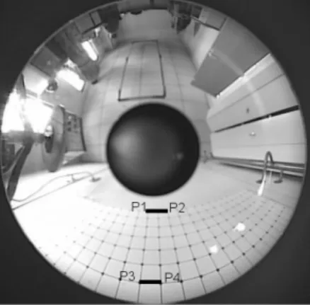
This chapter has presented the main tools used to localize a robot and reconstruct the scene from a 2D or 3D visual sensor. All approaches are based on the same steps. When only 2D information are provided, it is necessary to detect feature points, to match them, to deduce the camera motion, and to make a bundle adjustment on several acquisitions. On the other hand, if the visual sensor is able to produce 3D data, an ICP can simply be performed. We have studied here the case of a perspective camera model but the epipolar geometry is also valid in the case of a wide-angle image with a single point of view [13] (spherical, catadioptric : parabolic mirror + spelling camera, hyperbolic mirror + perspective camera...) but also fisheye [9] so the approaches discussed can be easily adapted to these cameras. Nevertheless, the features

Figure 9: Catadioptric image :d(P 1, P 2) = d(P 3, P 4)whenP 1does not have physically the same influence onP 2than

P 3onP 4.

extraction part must be adapted to this type of camera since traditional image processing (filtering, convolution) does not take into account the strong distortions present in these images (Fig 9). Some works dealt with these problems [10],[7] but it is still ongoing [2].

Concerning visual odometry, many works have been published on this topic and the estimation of the essential matrix is now well controlled. Recently, researchers have focused on reducing the number of characteristic points needed to estimate the camera motion using additional information on scene structure or camera orientation. This makes the estimation more robust to noise in the images and faster [12], [32].

In this chapter, we focused exclusively on fixed scenes. Nevertheless, when there are few moving points in the scene, the methods remain valid by integrating a robust approach such as RANSAC or M-estimator. But if the scene has many moving objects, the approaches have to be reviewed. Recently, some works related to motion estimation and 3D reconstruction on strongly dynamic scene have been published [18],[4],[38]. Finally, when the 3D scene is composed of non rigid motion, the problem becomes more challenging and still an open problem even if some works tackle this problem [33].

B

IBLIOGRAPHY

[1] Sameer Agarwal, Noah Snavely, Ian Simon, Steven M Seitz, and Richard Szeliski. Building rome in a day. In Computer Vision, 2009 IEEE 12th International Conference on, pages 72–79, 2009.

[2] Fatima Aziz, Ouiddad Labbani-Igbida, Amina Radgui, and Ahmed Tamtaoui. Generic spatial-color metric for scale-space processing of catadioptric images. Computer Vision and Image Understanding, 176:54–69, 2018.

[3] Simon Baker and Iain Matthews. Lucas-kanade 20 years on: A unifying framework. International journal of computer vision, 56(3):221–255, 2004.

[4] Ioan Andrei Bârsan, Peidong Liu, Marc Pollefeys, and Andreas Geiger. Robust dense mapping for large-scale dynamic environments. In 2018 IEEE International Conference on Robotics and Automation (ICRA), pages 7510–7517, 2018. [5] Herbert Bay, Tinne Tuytelaars, and Luc Van Gool. Surf: Speeded up robust features. In European conference on

computer vision, pages 404–417, 2006.

[6] Paul J Besl and Neil D McKay. Method for registration of 3-d shapes. In Sensor Fusion IV: Control Paradigms and Data Structures, volume 1611, pages 586–607, 1992.

[7] Iva Bogdanova, Xavier Bresson, Jean-Philippe Thiran, and Pierre Vandergheynst. Scale space analysis and active contours for omnidirectional images. IEEE Transactions on Image Processing, 16(7):1888–1901, 2007.

[8] J-Y Bouguet. Camera calibration toolbox for matlab. http://www. vision. caltech. edu/bouguetj/calib_doc/index. html, 2004.

[9] Jonathan Courbon, Youcef Mezouar, Laurent Eckt, and Philippe Martinet. A generic fisheye camera model for robotic applications. In Intelligent Robots and Systems, 2007. IROS 2007. IEEE/RSJ International Conference on, pages 1683–1688, 2007.

[10] Cédric Demonceaux, Pascal Vasseur, and Yohan Fougerolle. Central catadioptric image processing with geodesic metric. Image and Vision Computing, 29(12):840–849, 2011.

[11] David Fleet and Yair Weiss. Optical flow estimation. In Handbook of mathematical models in computer vision, pages 237–257. Springer, 2006.

[12] Friedrich Fraundorfer, Petri Tanskanen, and Marc Pollefeys. A minimal case solution to the calibrated relative pose problem for the case of two known orientation angles. In European Conference on Computer Vision, pages 269–282, 2010.

[13] Christopher Geyer and Kostas Daniilidis. A unifying theory for central panoramic systems and practical implications. In European conference on computer vision, pages 445–461, 2000.

[14] Jungong Han, Ling Shao, Dong Xu, and Jamie Shotton. Enhanced computer vision with microsoft kinect sensor: A review. IEEE transactions on cybernetics, 43(5):1318–1334, 2013.

[15] Chris Harris and Mike Stephens. A combined corner and edge detector. In Alvey vision conference, volume 15, pages 10–5244, 1988.

[16] Berthold KP Horn and Brian G Schunck. Determining optical flow. Artificial intelligence, 17(1-3):185–203, 1981. [17] Shahram Izadi, David Kim, Otmar Hilliges, David Molyneaux, Richard Newcombe, Pushmeet Kohli, Jamie Shotton,

Steve Hodges, Dustin Freeman, Andrew Davison, et al. Kinectfusion: real-time 3d reconstruction and interaction using a moving depth camera. In Proceedings of the 24th annual ACM symposium on User interface software and technology, pages 559–568, 2011.

[18] Cansen Jiang, Danda Pani Paudel, Yohan Fougerolle, David Fofi, and Cedric Demonceaux. Static and dynamic objects analysis as a 3d vector field. In 3D Vision (3DV), 2017 International Conference on, pages 234–243, 2017.

[19] Christian Kerl, Jurgen Sturm, and Daniel Cremers. Dense visual slam for rgb-d cameras. In Intelligent Robots and Systems (IROS), 2013 IEEE/RSJ International Conference on, pages 2100–2106, 2013.

[20] Stefan Leutenegger, Margarita Chli, and Roland Y Siegwart. Brisk: Binary robust invariant scalable keypoints. In Computer Vision (ICCV), 2011 IEEE International Conference on, pages 2548–2555, 2011.

[21] David G Lowe. Object recognition from local scale-invariant features. In Computer vision, 1999. The proceedings of the seventh IEEE international conference on, volume 2, pages 1150–1157, 1999.

[22] Bruce D Lucas, Takeo Kanade, et al. An iterative image registration technique with an application to stereo vision. 1981. [23] Renato Martins, Eduardo Fernandez-Moral, and Patrick Rives. Adaptive direct rgb-d registration and mapping for large

motions. In Asian Conference on Computer Vision, pages 191–206, 2016.

[24] Hans P Moravec. Obstacle avoidance and navigation in the real world by a seeing robot rover. Technical report, STANFORD UNIV CA DEPT OF COMPUTER SCIENCE, 1980.

[25] Jorge J Moré. The levenberg-marquardt algorithm: implementation and theory. In Numerical analysis, pages 105–116. Springer, 1978.

[26] Raul Mur-Artal and Juan D Tardós. Orb-slam2: An open-source slam system for monocular, stereo, and rgb-d cameras. IEEE Transactions on Robotics, 33(5):1255–1262, 2017.

[27] David Nistér. An efficient solution to the five-point relative pose problem. IEEE transactions on pattern analysis and machine intelligence, 26(6):756–770, 2004.

[28] François Pomerleau, Francis Colas, Roland Siegwart, et al. A review of point cloud registration algorithms for mobile robotics. Foundations and Trends® in Robotics, 4(1):1–104, 2015.

[29] Edward Rosten and Tom Drummond. Machine learning for high-speed corner detection. In European conference on computer vision, pages 430–443, 2006.

[30] Ethan Rublee, Vincent Rabaud, Kurt Konolige, and Gary Bradski. Orb: An efficient alternative to sift or surf. In Computer Vision (ICCV), 2011 IEEE international conference on, pages 2564–2571, 2011.

[31] Giovanna Sansoni, Marco Trebeschi, and Franco Docchio. State-of-the-art and applications of 3d imaging sensors in industry, cultural heritage, medicine, and criminal investigation. Sensors, 9(1):568–601, 2009.

[32] Olivier Saurer, Pascal Vasseur, Rémi Boutteau, Cédric Demonceaux, Marc Pollefeys, and Friedrich Fraundorfer. Homography based egomotion estimation with a common direction. IEEE transactions on pattern analysis and machine intelligence, 39(2):327–341, 2017.

[33] Miroslava Slavcheva, Maximilian Baust, and Slobodan Ilic. Sobolevfusion: 3d reconstruction of scenes undergoing free non-rigid motion. In Proceedings of the IEEE Conference on Computer Vision and Pattern Recognition, pages 2646–2655, 2018.

[34] Shuyang Sun, Zhanghui Kuang, Lu Sheng, Wanli Ouyang, and Wei Zhang. Optical flow guided feature: a fast and robust motion representation for video action recognition. In Proceedings of the IEEE conference on computer vision and pattern recognition, pages 1390–1399, 2018.

[35] Bill Triggs, Philip F McLauchlan, Richard I Hartley, and Andrew W Fitzgibbon. Bundle adjustment?a modern synthesis. In International workshop on vision algorithms, pages 298–372, 1999.

[36] Yi-Hsuan Tsai, Ming-Hsuan Yang, and Michael J Black. Video segmentation via object flow. In Proceedings of the IEEE Conference on Computer Vision and Pattern Recognition, pages 3899–3908, 2016.

[37] Tinne Tuytelaars, Krystian Mikolajczyk, et al. Local invariant feature detectors: a survey. Foundations and trends® in computer graphics and vision, 3(3):177–280, 2008.

[38] Minh Vo, Srinivasa G Narasimhan, and Yaser Sheikh. Spatiotemporal bundle adjustment for dynamic 3d reconstruction. In Proceedings of the IEEE Conference on Computer Vision and Pattern Recognition, pages 1710–1718, 2016. [39] Oliver Wasenmüller and Didier Stricker. Comparison of kinect v1 and v2 depth images in terms of accuracy and

precision. In Asian Conference on Computer Vision, pages 34–45, 2016.

[40] Simon Zingg, Davide Scaramuzza, Stephan Weiss, and Roland Siegwart. Mav navigation through indoor corridors using optical flow. In Robotics and Automation (ICRA), 2010 IEEE International Conference on, pages 3361–3368, 2010.