HAL Id: hal-01341015
https://hal-amu.archives-ouvertes.fr/hal-01341015
Submitted on 23 Feb 2017
HAL is a multi-disciplinary open access
archive for the deposit and dissemination of
sci-entific research documents, whether they are
pub-lished or not. The documents may come from
teaching and research institutions in France or
abroad, or from public or private research centers.
L’archive ouverte pluridisciplinaire HAL, est
destinée au dépôt et à la diffusion de documents
scientifiques de niveau recherche, publiés ou non,
émanant des établissements d’enseignement et de
recherche français ou étrangers, des laboratoires
publics ou privés.
Two Measures for the Homology Groups of Binary
Volumes
Aldo Gonzalez-Lorenzo, Alexandra Bac, Jean-Luc Mari, Pedro Real
To cite this version:
Aldo Gonzalez-Lorenzo, Alexandra Bac, Jean-Luc Mari, Pedro Real. Two Measures for the Homology
Groups of Binary Volumes. 19th IAPR International Conference on Discrete Geometry for Computer
Imagery (DGCI 2016), Apr 2016, Nantes, France. pp.154-165, �10.1007/978-3-319-32360-2_12�.
�hal-01341015�
Two Measures for the Homology Groups
of Binary Volumes
Aldo Gonzalez-Lorenzo1,2, Alexandra Bac1, Jean-Luc Mari1, and Pedro Real2
1
Aix-Marseille University, CNRS, LSIS UMR 7296, Marseille (France)
2
University of Seville, Institute of Mathematics IMUS, Seville (Spain)
Abstract. Given a binary object (2D or 3D), its Betti numbers char-acterize the number of holes in each dimension. They are obtained alge-braically, and even though they are perfectly defined, there is no unique way to display these holes. We propose two geometric measures for the holes, which are uniquely defined and try to compensate the loss of geo-metric information during the homology computation: the thickness and the breadth. They are obtained by filtering the information of the per-sistent homology computation of a filtration defined through the signed distance transform of the binary object.
1
Introduction
Homology computation is a very useful tool for the classification and the under-standing of binary objects in a rigorous way. It provides a class of descriptors summarizing the basic structure of the considered shape.
A binary object is a set X ⊂ Zd together with a connectivity relation. We will assume through this paper that X is a volume (d = 3) and the elements of X will be called voxels. However, the generalization to higher dimensions is direct.
Roughly speaking, homology deals with the “holes” of an object. Holes can be classified by dimensions: 0-holes correspond to connected components, 1-holes to tunnels or handles and 2-holes to cavities. When computing homology, we usually expect to find the number of these holes (called the Betti numbers) and a representative of each hole (called representative cycle of a homology generator). Nevertheless, the homology computation works at an abstract level (the chain complex) which ignores the embedding of the object. Thus, the geometry of the object is in some way neglected.
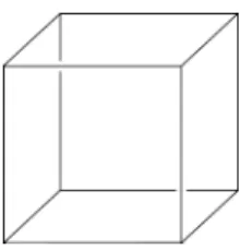
Moreover, holes are difficult to visualize. We can know how many they are, but not where they are. This is due to the fact that in homology computation, a choice for determining a linearly independent set of holes must be done. This is something difficult to apprehend: for instance, we remind that a cube with its interior and faces removed (as depicted in Fig. 1) contains five 1-holes instead of six.
The aim of this paper is to endow Betti numbers with an additional informa-tion containing a geometric interpretainforma-tion. We define two measures—thickness
Fig. 1.There are only five 1-holes in this object, and there is no natural way to state where they are.
and breadth—which, unlike homology generators, are uniquely determined by the object and can be used as concise topology descriptors. They are obtained through the persistent homology of the filtration induced by the signed distance transform of the volume.
Previous efforts have been made to combine homology and geometry. We cite herein some works that are related to our problem. Erickson and Whittle-sey founded an algorithm in [EW05] that computes the shortest base for the first homology group for oriented 2-manifolds. Dey et al. [DFW13] developed a similar work, but also classifying the 1-holes into tunnels and handles. Chen and Freedman [CF10] measured the 1-holes of a complex by the “length” of the homology generators and they also gave an algorithm to compute the smallest set of homology generators. Zomorodian and Carlsson introduced the localized homology in [ZC08], which allows to locate each homology class in a subset of a given cover. This cover, or collection of subcomplexes whose union contains the complex, successfully give a geometric sense to the Betti numbers.
Contributions
We define two geometric measures that enrich the Betti numbers of a binary volume. They are uniquely defined up to a choice of connectivity relation and distance. They can be computed through a distance transform and persistent homology, so it has matrix multiplication complexity over the number of voxels in the bounding box of the volume. These measures can be considered as pairs of numbers associated to each homology generator but also visualized as three-dimensional balls on the volume.
2
Preliminaries
2.1 Cubical Complexes and Homology
Cubical Complex — This section is derived from [KMM04]. For a deeper un-derstanding of these concepts, the reader can refer to it. An elementary interval is an interval of the form [k, k + 1] or a degenerate interval [k, k], where k ∈ Z. An elementary cube in Rn is the Cartesian product of n elementary intervals,
and the number of non-degenerate intervals in this product is its dimension. An elementary cube of dimension q will be called q-cube.
Given two elementary cubes σ and τ , we say that σ is a face of τ if σ ⊂ τ . It is a primary face if the difference of their dimensions is 1. Similarly, σ is a coface of τ if σ ⊃ τ . A cubical complex is a set of elementary cubes with all of their faces. The boundary of an elementary cube is the collection of its primary faces.
Chain Complex — A chain complex (C∗, d∗) is a sequence of groups C0, C1, . . . (called chain groups) and homomorphisms d1 : C1→ C0, d2 : C2 → C1, . . . (called differential or boundary operators) such that dq−1dq= 0, ∀q > 0.
Given a cubical complex, we define its chain complex as follows:
– Cq is the free group generated by the q-cubes of the complex;
– dq gives the “algebraic” boundary, which is the linear operator that maps every q-cube to the sum of its primary faces.
The elements of the chain group Cq, which are formal sums of q-cubes with coefficients in Z2, are called q-chains. They can be seen as sets of cubes of the same dimension.
Homology Groups — A q-chain x is a cycle if dq(x) = 0, and a boundary if x = dq+1(y) for some (q+1)-chain y. By the property dq−1dq = 0, every boundary is a cycle, but the reverse is not true: a cycle which is not a boundary contains a “hole”. The th homology group of the chain complex (C∗, d∗) contains the q-dimensional “holes”: H(C)q = ker(dq)/im(dq+1). This set is a finitely generated group, so there is a “base” typically formed by the holes of the cubical complex. Since our ring of coefficients is Z2, this group is isomorphic to Zβq and βq is the
q-th Betti number.
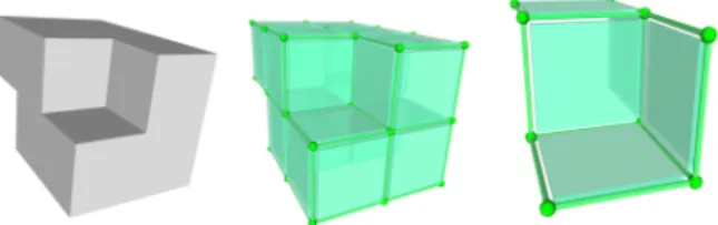
Cubical complex associated to a binary volume — Given a binary volume, we can define two different associated cubical complexes encoding the 6 or the 26-connectivity relation.
– Primal associated cubical complex (26-connectivity): every voxel x = (x1, x2, x3) generates the 3-cube [x1, x1+ 1] × [x2, x2+ 1] × [x3, x3+ 1] and all its faces. – Dual associated cubical complex (6-connectivity): let us first adapt the no-tion of clique to our context. A d-clique is a maximal (in the sense of inclu-sion) set of voxels such that their intersection is a d-cube. First, for every voxel (in fact 3-clique) x = (x1, x2, x3) of the volume, we add the 0-cube σ = [x1] × [x2] × [x3]. Then, for every d-clique (d < 3) in the volume, we add to the cubical complex a (3 − d)-cube such that its vertices are the voxels of the d-clique.
These cubical complexes can be defined for any dimension. Figure 2 illustrates both complexes.
Fig. 2.Left: a binary volume. Center: its primal associated cubical complex. Right: its dual cubical complex
2.2 Persistent Homology
This section introduces the persistent homology. A more rigorous presentation can be found in [EH08] and the references therein.
A filtration is a finite (or countable) sequence of nested cubical complexes X1⊂ X2⊂ · · · Xn. It can also be described by a function f on the final complex Xn, which assigns to each q-cube the first index at which it appears in the complex. Since it is a sequence of cubical complexes, a cube cannot appear strictly before its faces, so the function f must verify
f (σ) ≤ f (τ ), ∀σ ⊂ τ (1) Therefore, a function f : X → R defined over a cubical complex is a filtration function if its image is a finite (or countable) set and if it satisfies Eq. (1). Given such a function, its filtration is the sequence Ff(X) = {Xi}ni=0, where a0< a1< · · · < an are the images of f and Xi= f−1(]−∞, ai]).
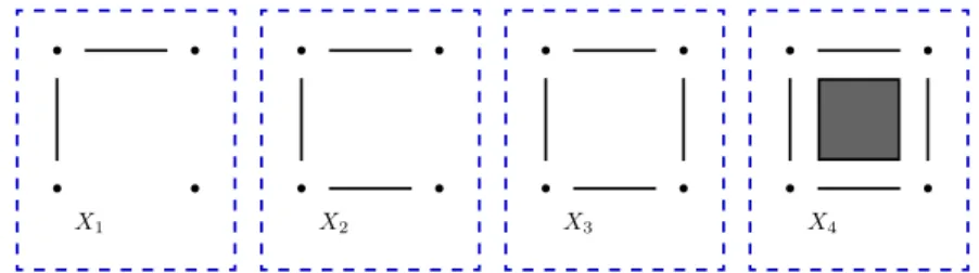
As illustrated in Fig. 3, the homology groups of the complex can evolve as “time” goes on. The persistence diagram [EH08, p. 3] records these changes: a q-hole being born in Xi and dying (or vanishing) in Xj is represented in the persistence diagram as the point (i, j). This is also called a P -interval in [ZC05]. A homology generator of Xn, which never dies, is represented by the point (i, ∞). The reader can find some persistence diagrams in Sect. 4. Persistent homology can also be visualized in terms of barcodes [Ghr08], where each point (i, j) is represented as an interval in the real line.
We can assign a pair of cubes (σi, σj) to each P -interval (i, j). The first cube creates the hole (e.g., a point in a new connected component or the edge that closes a handle) while the second one merges the hole into the set of boundaries (e.g., the edge that connects two connected components, or the square that fills a handle). The reader could try to find these pairs of cubes in the filtration described in Fig. 3.
There has been an extensive research in the computation of persistent homol-ogy. An algorithm in matrix multiplication time was introduced in [MMS11]. The algorithms present in [ZC05,MN13] have cubical worst-time complexity, but they seem to behave better in practice. An algorithm adapted for cubical complexes was developed in [WCV12].
b b b b X1 b b b b X2 b b b b X3 b b b b X4
Fig. 3.A filtration. X1: there are two 0-holes (connected components). X2: one 0-hole
dies. X3: a 1-hole is born. X3: that 1-hole dies.
Note that in this article we do not use ˇCech, Vietoris-Rips nor Alpha com-plexes, as it is usually done in the persistent homology literature. The filtrations considered are based on a function defined over a cubical complex.
2.3 Distance Transform
Given a binary volume X ⊂ Z3, its distance transform DTX is the map that sends every voxel x ∈ X to DTX(x) = miny∈Z3\Xd(x, y). It can be seen as
the radius of the maximal ball centered at x and contained in X. Note that we must consider one specific distance for the volume: Lp metrics such as the Manhattan distance (L1), the Euclidean distance (L2) or the chessboard distance (L∞); distances based on chamfer masks [Mon68,Bor84] or sequences of chamfer masks [MDKC00,NE09], etc.
There exist linear time algorithms for computing the Euclidean distance on nD binary objects [BGKW95,Hir96,MRH00,MQR03].
We can then consider the signed distance transform, which maps every voxel x ∈ X to −DTX(x) and x /∈ X to DTZ3\X(x).
3
The Two Measures
3.1 Motivation
The main motivation for this work comes from the desire of comparing binary volumes obtained from real acquisition of complex structures. Using mere Betti numbers for this objective can be ineffective, so we thought of enhancing this basic homological information by defining two geometry-aware measures for the holes.
In the following we give an intuitive introduction to the two new measures. We consider two binary images which are repeatedly eroded and dilated respectively, and we comment what happens to their homology groups. Then we figure out how we can treat this problem with persistent homology.
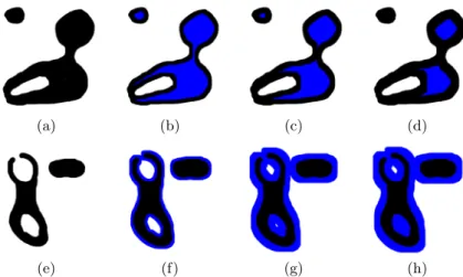
When we erode the image in Fig. 4-(a), we observe that a 1-hole disappears (Fig. 4-(b)), a 0-hole is created (Fig. 4-(c)) and a 0-hole disappears (Fig. 4-(d)).
(a) (b) (c) (d)
(e) (f) (g) (h)
Fig. 4.Two images being eroded and dilated. We can notice a change in its homology at every step.
On the other hand, when we dilate the image in Fig. 4-(e), a new 1-hole appears (Fig. 4-(f)), a 0-hole vanishes (Fig. 4-(g)) and a 1-hole disappears (Fig. 4-(h)).
Thanks to persistent homology, we can record these events. Given a binary volume X ⊂ [0, m1] × [0, m2] × [0, m3] ⊂ Z3, we build the associated primal (or dual) cubical complex K of the bounding box [0, m1] × [0, m2] × [0, m3]. Then we compute a filtration function f associated to the signed distance transform of X: the 3-cubes (0-cubes) are mapped to the value of their associated voxels (cf. Sect. 2.1). The image of the rest of the cubes is coherently assigned in order to produce a filtration, that is, each q-cube, for 0 ≤ q ≤ 2 (1 ≤ q ≤ 3), takes the minimum (maximum) value of its 3-dimensional cofaces (0-dimensional faces).
Let a0< a1 < · · · < ai = 0 < · · · < an be the different values of f over the volume. Thus, we can consider the filtration Ff(K):
X0= f−1(]−∞, a0]) ⊂ · · · ⊂ X ⊂ · · · ⊂ Xn= f−1(]−∞, an])
Let us now see how the previously described phenomena are encoded in the persistent homology of the filtration Ff(K). Note that the eroded images are now seen in reversed time:
– Fig. 4-(b): a 1-hole is born in negative time (1b–); – Fig. 4-(c): a 0-hole dies in negative time (0d–); – Fig. 4-(d): a 0-hole is born in negative time (0b–); – Fig. 4-(f): a 1-hole is born in positive time (1b+); – Fig. 4-(g): a 0-hole dies in positive time (0d+); – Fig. 4-(h): a 1-hole dies in positive time (1d+);
Since we are interested in the homology groups of the given volume, we only consider the persistent intervals that start at negative time and finish at positive time. We can give an intuitive and physical interpretation to those events.
0b– A 0-hole being born at time t0< 0 means that the maximal ball included in that connected component has radius −t0;
0d+ A 0-hole dying at time t0 > 0 means that the shortest distance between that connected component and any other is 2 · t0;
1b– A 1-hole being born at time t0 < 0 means that −t0 is the smallest radius needed for a ball included in X that, once removed, breaks or vanishes that hole;
1d+ A 1-hole dying at time t0> 0 means that the maximal ball that can pass through that hole has radius t0;
2b– Same as 1b–;
2d+ A 2-hole dying at time t0 > 0 means that the maximal ball that can fit inside that hole has radius t0;
Thus, for q = 1, 2, the time t at which a q-hole is born can be seen as the thickness of the hole, or how far it is from being destructible. We will call it thickness. Also, the time t at which a q-hole dies can be interpreted as a kind of size or breadth. We choose this second term, since the size of a 2-hole is better understood as the volume it covers or the area of its boundary. These two terms are not suitable for dimension 0, so we use the terms breadth (again) and separability respectively.
3.2 Definitions
Let X ⊂ [0, m1] × [0, m2] × [0, m3] ⊂ Z3
be a binary volume and d : Z3
→ R+a distance. Consider the signed distance transform
sDTX(x) = (
− min{d(x, y) : y /∈ X} , x ∈ X min{d(x, y) : y ∈ X} , x /∈ X
Depending on which connectivity relation we use for the volume, we build its as-sociated cubical complex K (cf. Sect. 2.1) and the filtration function fXinduced by sDTX (cf. Sect. 3.1).
The thickness and breadth of the q-holes of X are the pairs {(−ik, jk)}βq
k=1, where {(ik, jk)}
βq
k=1 are the P -intervals of the filtration fX such that ik < 0 and jk > 0 for all 1 ≤ k ≤ βq. We can represent these pairs as points in R2 in the thickness-breadth diagram.
The final step of the filtration is the full cubical complex associated to the bounding box of the volume. If the volume is not empty, as the bounding box has one connected component there exists a P -interval (−i, ∞) of dimension 0. We will represent this breadth pair as (−i, −1) in the thickness-breadth diagram. As a consequence, a volume has β0− 1 separation values. This is coherent with its interpretation, as there are only n − 1 shortest distances between n objects.
Note that the thickness-breadth pairs are uniquely defined for the filtration and they only depend on the connectivity relation of the volume and the distance considered.
3.3 Visualization
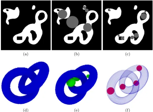
The breadth and thickness values of a volume can be visualized in terms of balls, as it was suggested in Sect. 3.1. Given a thickness-breadth pair (i, j) with its (non-unique) associated pair of cubes (σ, τ ) (cf. Sec. 2.2), we can also assign a pair of voxels (p, q) to them. For the primal (dual) associated cubical complex, according to its construction (cf. Sect 2.1), we choose any coface of dimension 3 (face of dimension 0) with the same image under f for each cube and we take its associated voxel in the original volume. We call these voxels, which are not unique, v(i) and v(j).
Therefore, for each hole we can visualize its thickness by the ball centered at v(i) with radius i, and similarly for its breadth. Figure 5 illustrates this procedure.
(a) (b) (c)
(d) (e) (f)
Fig. 5.Example of visualization of the thickness and the breadth through balls. Top: a binary image (a) with the balls of H0 (b) and H1 (c). Bottom: a binary volume (d)
which contains two chained volumetric tori, its breadth (e) and its thickness balls (f) of dimension 0 and 1.
4
Results
Our implementation for computing the breadth and the thickness uses the DGtal library [DGt] for the distance transform and the Perseus software [Nan] for the
persistent homology. In order to obtain the centers of the balls, we developed a specific software. The following volumes were voxelized with the Binvox software [Min,NT03].
Figure 6 shows some examples of thickness-breadth diagrams. For each bi-nary volume, we show the diagram containing the thickness-breadth pairs of the homology groups H0 (red circles), H1 (green triangles) and H2 (blue squares). Note that we represent the pairs (i, ∞), associated to the “broadest” connected component of the volume, as (i, −1).
We can appreciate the fractal structure of the Menger sponge after three iterations in its diagram. There are only three possible values for the breadth and the thickness: (1,30
+1 2 ), (1, 31 +1 2 ) and (1, 33 +1
2 ). For the lamp [Rey15], we can easily recognize a lot of similar holes and a bigger one, which traverses the volume along the z-axis. The small 2-hole follows from a discretization error. The diagram of the Colosseum volume [Gas15] presents a regular shape. All the 1-holes (i.e., the doors) have similar measures, except for one which has greater thickness. It corresponds to the ground floor concentric corridor.
Figure 7 illustrates the pertinence of the visualization described in Sect. 3.3. More examples are available on [GL].
5
Conclusion and Future Work
This paper introduces a concise and rigorous geometrical and topological infor-mation for binary volumes that extends the Betti numbers. This could be used for a statistical analysis of the volume or a better understanding of its topological features.
An interesting issue that should be addressed in the near future is the stability of this definition. Are the breadth and thickness stable under small perturbations of the volume? How much do these values change when we consider different connectivity relations or distances?
In addition, it seems that the intersection of the thickness and breadth balls with the volume could provide a heuristic for computing geometry-aware homol-ogy and cohomolhomol-ogy generators.
References
[BGKW95] H. Breu, J. Gil, D. Kirkpatrick, and M. Werman. Linear time Euclidean distance transform algorithms. IEEE Transactions on Pattern Analysis
and Machine Intelligence, 17:529–533, 1995.
[Bor84] G. Borgefors. Distance transformations in arbitrary dimensions. Computer
Vision, Graphics, and Image Processing, 27(3):321 – 345, 1984.
[CF10] C. Chen and D. Freedman. Measuring and computing natural generators for homology groups. Computational Geometry, 43(2):169–181, 2010. Spe-cial Issue on the 24th European Workshop on Computational Geometry (EuroCG’08).
[DFW13] T. K. Dey, F. Fan, and Y. Wang. An efficient computation of handle and tunnel loops via Reeb graphs. ACM Trans. Graph., 32(4):32:1–32:10, 2013.
Fig. 6.Left: three binary volumes. Right: their thickness-breadth diagrams. 0-holes are represented by red circles, 1-holes by green triangles and 2-holes by blue squares.
Fig. 7.Examples of thickness (red) and breadth (green) balls. Top: Fertility volume, available by AIM@SHAPE with the support of M. Couprie. Bottom: Menger sponge, available on [GL].
[EH08] H. Edelsbrunner and J. Harer. Persistent homology – a survey. In J. Pach J. E. Goodman and R. Pollack, editors, Surveys on Discrete and
Computa-tional Geometry: Twenty Years Later, volume 453, pages 257–282, Provi-dence, Rhode Island, 2008. Amer. Math. Soc., Contemporary Mathematics. [EW05] J. Erickson and K. Whittlesey. Greedy optimal homotopy and homology generators. In Proceedings of the Sixteenth Annual ACM-SIAM Symposium
on Discrete Algorithms, SODA ’05, pages 1038–1046, Philadelphia, PA, USA, 2005. Society for Industrial and Applied Mathematics.
[Gas15] J. Gaspard. Roman colosseum completley detailed see the world. https://www.thingiverse.com/thing:962416, Aug. 2015. Creative Commons License.
[Ghr08] R. Ghrist. Barcodes: The persistent topology of data. Bulletin of the
American Mathematical Society, 45:61–75, 2008.
[GL] A. Gonzalez-Lorenzo. http://aldo.gonzalez-lorenzo.perso.luminy.univ-amu.fr/measures.html, Accessed 20/10/2015.
[Hir96] Tomio Hirata. A unified linear-time algorithm for computing distance maps. Information Processing Letters, 58(3):129–133, 1996.
[KMM04] T Kaczynski, K Mischaikow, and M Mrozek. Computational Homology, volume 157, chapter 2, 7, pages 255–258. Springer, 2004.
[MDKC00] J. Mukherjee, P.P. Das, M. Aswatha Kumar, and B.N. Chatterji. On approximating Euclidean metrics by digital distances in 2D and 3D. Pattern
[Min] Patrick Min. Binvox, 3D mesh voxelizer. http://www.cs.princeton.edu/ min/binvox/, Accessed 07/10/2015. [MMS11] N. Milosavljevi´c, D. Morozov, and P. Skraba. Zigzag persistent homology
in matrix multiplication time. In Proceedings of the Twenty-seventh Annual
Symposium on Computational Geometry, SoCG ’11, pages 216–225, New York, NY, USA, 2011. ACM.
[MN13] K. Mischaikow and V. Nanda. Morse theory for filtrations and efficient computation of persistent homology. Discrete and Computational
Geome-try, 50(2):330–353, 2013.
[Mon68] U. Montanari. A method for obtaining skeletons using a quasi-Euclidean distance. J. ACM, 15(4):600–624, October 1968.
[MQR03] Jr. Maurer, C.R., Rensheng Qi, and V. Raghavan. A linear time algorithm for computing exact Euclidean distance transforms of binary images in arbitrary dimensions. IEEE Transactions on Pattern Analysis and Machine
Intelligence, 25(2):265–270, 2003.
[MRH00] A. Meijster, J.B.T.M. Roerdink, and W.H. Hesselink. A general algorithm for computing distance transforms in linear time. In John Goutsias, Luc Vincent, and DanS. Bloomberg, editors, Mathematical Morphology and its
Applications to Image and Signal Processing, volume 18 of Computational
Imaging and Vision, pages 331–340. Springer US, 2000.
[Nan] V. Nanda. Perseus, the persistent homology software. http://www.sas.upenn.edu/ vnanda/perseus, accessed 07/10/2015. [NE09] N. Normand and P. ´Evenou. Medial axis lookup table and test
neigh-borhood computation for 3D chamfer norms. Pattern Recognition, 42(10):2288–2296, 2009. Selected papers from the 14th {IAPR} Interna-tional Conference on Discrete Geometry for Computer Imagery 2008. [NT03] F. S. Nooruddin and G. Turk. Simplification and repair of polygonal models
using volumetric techniques. IEEE Trans. Vis. Comput. Graph., 9(2):191– 205, 2003.
[Rey15] A. Reynolds. Radiant blossom. https://www.thingiverse.com/thing:978768, Aug. 2015. Creative Commons License.
[WCV12] H. Wagner, C. Chen, and E. Vu¸cini. Efficient computation of persistent homology for cubical data. In Ronald Peikert, Helwig Hauser, Hamish Carr, and Raphael Fuchs, editors, Topological Methods in Data Analysis and
Visualization II, Mathematics and Visualization, pages 91–106. Springer Berlin Heidelberg, 2012.
[ZC05] A. Zomorodian and G. Carlsson. Computing persistent homology. Discrete
and Computational Geometry, 33(2):249–274, 2005.
[ZC08] A. Zomorodian and G. Carlsson. Localized homology. Computational