HAL Id: hal-03150538
https://hal-amu.archives-ouvertes.fr/hal-03150538
Submitted on 24 Feb 2021
HAL is a multi-disciplinary open access
archive for the deposit and dissemination of
sci-entific research documents, whether they are
pub-lished or not. The documents may come from
teaching and research institutions in France or
abroad, or from public or private research centers.
L’archive ouverte pluridisciplinaire HAL, est
destinée au dépôt et à la diffusion de documents
scientifiques de niveau recherche, publiés ou non,
émanant des établissements d’enseignement et de
recherche français ou étrangers, des laboratoires
publics ou privés.
Tidal stream turbine control: An active disturbance
rejection control approach
Zhibin Zhou, Seifeddine Ben Elghali, Mohamed Benbouzid, Yassine Amirat,
Elhoussin Elbouchikhi, Gilles Feld
To cite this version:
Zhibin Zhou, Seifeddine Ben Elghali, Mohamed Benbouzid, Yassine Amirat, Elhoussin Elbouchikhi,
et al.. Tidal stream turbine control: An active disturbance rejection control approach. Ocean
Engi-neering, Elsevier, 2020, 202, pp.107190. �10.1016/j.oceaneng.2020.107190�. �hal-03150538�
Tidal Stream Turbine Control: An Active Disturbance
1
Rejection Control Approach
2 3
Zhibin Zhou
1, Seifeddine Ben Elghali
2, Mohamed Benbouzid
3,4, Yassine Amirat
1, Elhoussin Elbouchikhi
1, and Gilles
4
Feld
15
1ISEN Yncréa Ouest, UMR CNRS 6027 IRDL, Brest, France
6
2Aix-Marseille University, UMR CNRS 7020 LIS, Marseille, France
7
3University of Brest, UMR CNRS 6027 IRDL, 29238 Brest, France
8
4Shanghai Maritime University, 201306 Shanghai, China
9
[email protected], [email protected], [email protected], [email protected],
10
[email protected], [email protected]
11 12
Abstract— As an emerging technology to harness the marine current energy, tidal stream turbine (TST) systems have been developed due to
13
high predictability and energy density in tidal current resources. However, considering that various challenges such as swell disturbances,
14
unknown disturbances, or parameter uncertainties may deteriorate the system performance, it is interesting to investigate alternative control
15
strategies to the conventional proportional-integral (PI) controls. In this paper, the active disturbance rejection control (ADRC) approach is
16
proposed to replace PI controllers in the conventional generator-side control scheme. In this approach, two ADRC schemes (cascaded and
17
second-order ADRC strategies) are respectively applied and compared to achieve MPPT under current velocity and turbine torque disturbances.
18
Performances of the proposed ADRC approaches are compared to PI and sliding mode control strategies. Energy production during swell wave
19
disturbance is also evaluated under these control strategies. The comparisons show that the cascaded ADRC has better performance than the
20
second-order approach. Moreover, the cascaded ADRC is tested under parameter variations to evaluate its robustness. The carried out
21
simulation-based comparative study shows the effectiveness and advantages of the cascaded ADRC strategy over conventional PI controller in
22
terms of fast convergence, overshoots elimination, and improved robustness under disturbances and parameter uncertainties.
23 24
Keywords— Tidal stream turbine, disturbance rejection control, maximum power point tracking, robustness.
25
I. INTRODUCTION 26
Tidal stream turbine (TST) generation systems, based on similar principles of wind power systems, have been developed to 27
generate electricity from tidal-driven currents during the last decades. Advantages of TST generation systems are related to the 28
high predictability (in hourly time scale) and high energy density of the tidal-driven currents [1-2]. Although challenges such as 29
submarine installation and maintenance do exit, TST generation systems are still considered to be a promising power supplying 30
solution for some remote islands or coastal areas. In fact, various demonstrative TST projects have been successfully 31
industrialized and they are entering the pre-commercial stage [3-4]. For achieving compact structure and reducing maintenance 32
requirements, several TST projects adopt turbines with nonpitchable blades and choose permanent magnet synchronous machine 33
as generator [5]. 34
The power harnessed by a TST is generally proportional to the cubic marine current velocity and the turbine power coefficient. 35
For a turbine with fixed-pitch blades, the turbine power coefficient (Cp) depends on the tip speed ratio (TSR), which can be
36
controlled by the generator rotational speed. Therefore, speed control in TST generation system can be necessary in order to 37
capture maximum power under the varying marine current speed. A previous study in [6] shows that under strong swell wave 38
disturbances, a speed control with filter-based reference or a torque-based control can achieve smoother produced power. 39
Z. Zhou, S. Benelghali, M. Benbouzid, Y. Amirat, E. Elbouchikhi, G. Feld, “Tidal stream turbine control: An active disturbance rejection control approach,” Ocean Engineering, vol.202, 107190, pp. 1-9, march 2020
However, in that work only classical proportional-integral (PI) controllers are used and other kind of disturbances such as sudden 40
current flow velocity change and unpredictable turbine mechanical torque changes are not considered. 41
Although PID control is the most popular control strategy in industrial applications due to its simple structure and relative easy 42
parameter tuning, it may suffer several drawbacks such as: 1) the controller implementation is often done without the derivative 43
part (D) due to noise sensitivity; 2) slow response or overshoot caused by the integration action; 3) controller parameter tuning 44
usually requires accurate plant model and parameters, which may be unavailable or present uncertainties under different 45
operation conditions. To improve the transient performance of PID controllers, system identification and intelligent techniques 46
are introduced [7]. Fuzzy PID controllers can have better performances with adaptive controller gains, however the design of 47
membership function and rule sets could be difficult and complex [8-9]. In modern control, there are several advanced control 48
strategies, which are interesting. The model predictive control (MPC) and linear quadratic regulator (LQR) require analysis of 49
the space-state model of the plant. They have good performance around the steady-state operating point but are not robust and 50
could be sensitive to unmodeled dynamics and external disturbances [10-11]. As a group of variable structure controllers, higher-51
order sliding (HOSM) controllers are considered as a powerful control tool for nonlinear systems under parameter uncertainties. 52
HOSM is developed to reduce chattering, which is caused by unmodeled dynamics that increase the relative degree of the plant 53
[12]. In various HOSM control laws, high-order time derivatives of the sliding variable are often required. However, measuring 54
high order derivatives in practice is often with high noises and not feasible. In this case, high-order finite-time convergent 55
observer based on the symbolic function should be used [13]. The choice of the control laws and parameter tuning of the HOSM 56
could be difficult when the boundary conditions of the variation range or variation rate of certain system parameters are 57
unavailable. 58
In [14-16], a relatively new design structure for controllers, namely active disturbance rejection control (ADRC), was 59
proposed. ADRC is not based on plant model analysis, because system behaviors could change unexpectedly in practice under 60
disturbances and the plant models may therefore become unreliable. As an emerging approach, ADRC uses a controller-observer 61
pair to treat external and internal disturbances, plant parameter variations or uncertainties as an element not to be modeled 62
analytically but to be rejected as a generalized “total disturbance”; in this way the control signal responds directly to cancel the 63
“total disturbance” and thus making the controller design almost model-free [17]. Linear ADRC (LADRC) enables to apply 64
parameter-tuning methods based on close-loop bandwidth and observer bandwidth according to desired frequency or time 65
domain performances [18-19]. However, the study in [20] shows that the limitation of sensor bandwidth could degrade the 66
closed-loop performance of the LARDC. Various parameter uncertainties and external disturbances exist in PM machines, a 67
comprehensive overview on disturbance and uncertainty estimation and attenuation (DUEA) techniques including ADRC is 68
given in [21]; it shows that DUEA has a better balance among performances compared to other robust control and adaption 69
control methods. In [22-23], ARDC are applied to the speed controller of PM machines, however PI controllers are still used in 70
the current loops. In a recent work [24], ADRC was applied on a laboratory-scaled small PM machine and compared to PI and 71
SM controls. Although the comparison carried out in [24] is of some interest, there were several issues such as the size of the 72
used PM machine that does not fit tidal stream turbine systems power level for deployment, ADRC was only applied in the speed 73
control loop, and the robustness issue has not been addressed while it is a critical issue in a marine context (i.e. parameter 74
variations). All these issues will be addressed in this work while a control alternative, namely a second-order ADRC approach, 75
will be developed and compared to the proposed cascaded ADRC approach. 76
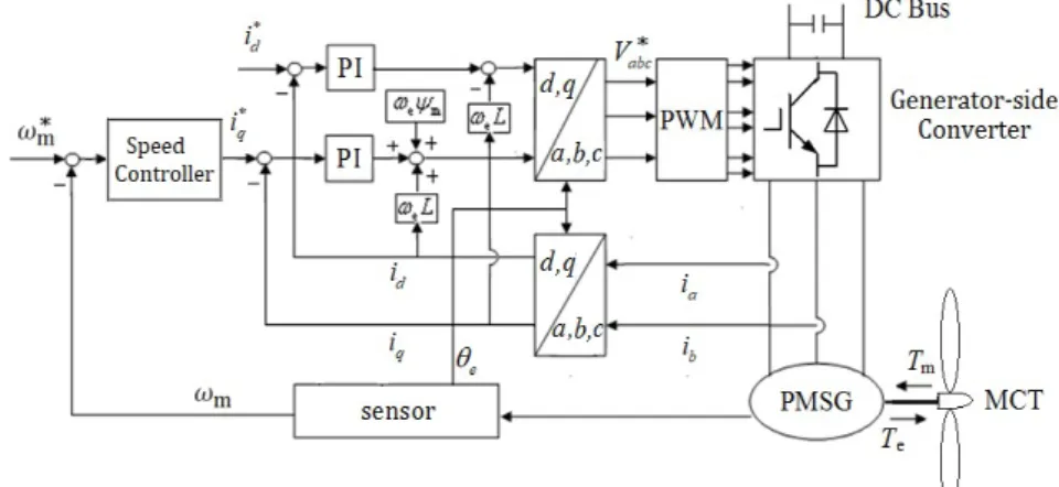
Figure 1 shows a classical double-loop control scheme of a permanent magnet synchronous generator (PMSG); the current 77
loop control is usually based on PI controllers; and the speed controller can be either PI controller or other advanced controller. 78
In order to fully benefit from the ADRC strategies advantages, an all-ADRC approach, as shown in Fig. 2, is proposed in this 79
work. In this approach, all the controllers both in speed and current loops are designed by ADRC strategies. In the proposed 80
cascaded ADRC approach, the decoupling terms in the classical PI current control loops are not needed and thus the dependence 81
of system parameters can be reduced. Using a higher order ADRC controller to combine the speed ADRC controller and the q-82
axis ADRC current controller can achieve a possible variant of this ADRC approach. 83
Nonlinear ARDC controllers are applied in this work to fully maintain the advantages of “large error, small gain; small error, 84
large gain” compared to LADRC. The proposed all-ADRC approach is applied to a 500 kW TST generation system to achieve 85
the MPPT task under different kinds of disturbances and parameter variations. 86
87
88
Fig. 1. Classical control scheme for a PMSG-based TST system.
89 90
91
Fig. 2. Proposed ADRC control scheme for a PMSG-based TST system.
92 93
In Section II, the PMSG-based TST system model and classical controller design for the TST generation system are presented. 94
Then, the proposed ADRC approach and the controller design are presented in Section III. In Section IV, simulation results of 95
different control strategies under tidal current speed and turbine torque disturbances are compared. Energy production 96
performance under swell effect is also presented. In Section V, parameter uncertainties are applied to verify the proposed ADRC 97
robustness. Section VI gives the conclusion. 98
II. CLASSICAL CONTROL FOR A TST SYSTEM 99
The mechanical power extracted by a TST can be calculated by the following equation. 100 101
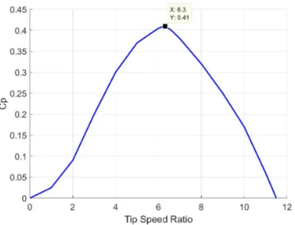
2 3 1 ρ π 2 p tide P C R V (1) 102In (1), the seawater density ρ and the turbine radius R are constants; Vtide is the velocity of marine tidal current; Cp is the
103
turbine power coefficient. For a given turbine, the Cp curve may be approximated as a function of the pitch angle and the tip
104
speed ratio . The considered TST is a fixed-pitch blade one, therefore Cp depends only on . For typical MCT prototypes, the
105
optimal Cp value is estimated to be in the range of 0.39-0.45 [3]. Figure 3 shows the Cp curve used in this work. The maximum
106
Cp value is 0.41, which corresponds to a tip speed ratio of 6.3. This value is considered as the optimal tip speed ratio (λopt = 6.3)
107
for obtaining the maximal Cp value under varying tidal current condition.
108 109
110
Fig. 3. Cp curve of the studied TST.
111 112
A basic MPPT control can be realized by controlling the generator speed to regulate the turbine rotational speed according to 113
tidal current velocity. The speed reference for the generator can be given by (2) for the considered direct-driven TST: 114 115 opt tide m V R (2) 116 117
For the PMSG, the d-q frame model is described by (3). 118 119 s e s e e m e p m m m e B m d ω dt d ω ω ψ dt 3 ψ ( t ) 2 d d d d d d q q q q q q q d d q d d q i v R i L L i i v R i L L i T n i L L i i J T T f (3) 120 121
In (3), vd, vq and id, iq are stator voltages and currents in the d-q axis respectively; Rs is the stator resistance; Ld, Lq are
122
inductances in the d-q axis (Ld = Lq = Ls for a non-salient machine is considered in this work); ωe, ωm are machine electrical and
123
mechanical speed; Te , Tm are respectively the machine electromagnetic and the mechanical torques; np is the generator pole pair
124
number; ψm is the flux linkage created by the rotor permanent magnets; J is the total system inertia and fB is the friction
125
coefficient associated to the mechanical drivetrain. A 500kW TST system is considered in this work and the system parameters 126
are given in the Appendix. 127
In the classical control scheme shown in Fig. 1, the current loop response is much faster than the speed response and the 128
current controller tuning is usually easier than the speed controller. Therefore, PI control are applied for the two current loops in 129
this section, and then two different control strategies – PI and sliding mode (SM) control will be applied to the speed controller. 130
The controllers should be well tuned to serve as a sound base for later comparison with the proposed ADRC strategies. 131
A. Proportional-Integral Control 132
The tuning of the two PI controllers (shown in Fig. 1) in the current loops is to be presented firstly. Same parameters can be 133
used for both PI current controllers due to the similar dynamics for id and iq loops. The open-loop transfer function of the PI
134
control based current loop can be expressed as: 135 136
0 ( 1) 1/ ( ) ( / ) 1 1 pc ic s ic s s I K s R G s s L R s T s (4) 137 138with Kpc and Kic1/icas the current-loop controller gains and TI(which is much smaller than the electrical time constant
139
Ls/Rs) as a small time constant standing for current sensor and power converter delays. Based on the dominant pole cancelation
140
method and with a desired damping factor (0.707 in this work) for the close-loop transfer function, the following controller gains 141
can be chosen for the current-loop PI controllers: 142 143
/ 2 ic s s pc s I ic K R L K R T K (5) 144 145The speed controller will generate the q-axis current reference iq
. The d-axis current reference d
ican be set to 0 for
146
maximizing the electromagnetic torque for a given stator current. The PI speed controller parameters can be tuned by many 147
ways, and in this work the non-symmetrical optimum method (NSOM) is chosen. As one analytical method, the NSOM relies on 148
a second-order approximated model of the plant with a generalized time constant (TQ1 /Q), which includes all the time delays
149
in the speed loop, and KQ, which represents the slope rate of open-loop step response. These two parameters can be deduced
150
from a series of step response tests in simulation or in practice. By the NSOM, the parameters of the PI speed controller can be 151
obtained from [25] as follows: 152 153 Q ps c Q c Q is c K K K (6) 154 155
In (6), the correcting gain fact γc is defined in terms of the desired resonant peak value Mc; the parameter αc is calculated by a
156
phase advance Δφ, which depends on γc. More details of the NSOM tuning procedure can be found in [26].
157
B. Sliding Mode Speed Control 158
To improve the PMSG speed control performance, HOSM can be applied [27-29]. In this work, the super-twisting sliding 159
mode control strategy is applied to the speed controller as an alternative to the PI one. The sliding variable is defined as the speed 160 tracking error, 161 162 1 m m s e (7) 163 164
and the controller output is calculated by 165 166
0.5 1 1 sign 1 2 sign 1 q u i K s s K s
(8) 167 168The lower limits of the gains K1 and K2 for the super-twisting control law can be calculated with bounding information of
certain parameters variation range and variation rate [30]. Generally, higher gains are needed to cover higher parameter 170
uncertainty and larger disturbances. In this work, K1 = 1200 and K2 = 500 are chosen for the studied TST system.
171
III. ADRC ALTERNATIVE APPROACH FOR THE TST SYSTEM 172
A. Active Disturbance Rejection Control 173
From the previous PI speed controller tuning procedure, it can be noted that the PI gains relay on the knowledge of plant 174
parameters or require some tests to obtain an approximate plant model. However, disturbances or nonlinear dynamics are not 175
considered in PI controller designs. 176
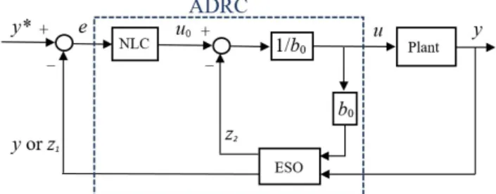
To overcome these drawbacks, ADRC uses a nonlinear controller (NLC) with an extended state observer (ESO) to obtain fast 177
convergence and effective disturbance rejection. A stand formulation for applying ADRC is based on a canonical state-space 178
expression of the plant with the “total disturbance” as an extended state variable. The ADRC controller order depends on the 179
derivative order of the target variable to be controlled [24]. The first-order derivation of the plant output y can be formulated by 180 181 1 1 x F b u y x (9) 182 183
In (9), u is the plant input, b is a constant, and F represents the total disturbance (which combines all the known dynamics and 184
unknown disturbances). Then, F is treated as an extended state variable x2 to be estimated by the ESO. The first-order ADRC
185
controller diagram is illustrated by Fig. 4. In this figure, e is the tracking error; b0 is a roughly estimated value of the constant b
186
of the plant described in (9); and the ESO has two outputs: z1 is an estimation of the plant output y; and z2 is the estimated total
187
disturbance F. 188
189
Fig. 4. General first-order ADRC control diagram.
190 191
The nonlinear function called fal is applied in the ADRC, 192 193 1 sign( ), ( , , ) , x x x fal x x x (10) 194 195
with x as the main input representing some kind of error information; 0 < α < 1 enables the function value to have a reducing 196
effect with large x input and δ > 0 introduces a linear zone to avoid too big function value for small x around 0. 197
The ESO of the ADRC can then be constructed as 198 199
1 1 2 0 1 1 2 2 2 , , , , z y z z b u fal z fal (11) 200with β1, β2 as the ESO gains. The NLC is given as u0 k fal e1 ( , 0, ), with k1 as the controller gain. The ADRC controller
201
output is u
u0z2
/b0. It is also possible to move the block 1/b0 on the z2 signal channel in Fig. 4 and thus making the202
controller output u u 0z b2/ 0. This could be helpful to reduce the NLC output u0 and its controller gain k1, when the constant
203
b0 is very large.
204
B. Cascaded ADRC Control 205
In the proposed cascaded ADRC control for the tidal stream turbine generation system (Fig. 2), the current loop ADRC 206
controllers are constructed based on the first-order derivation of the d-q axis currents. 207 208
m
1 1 1 1 ψ d s d e q q d d d q s q e d d e q q q i R i L i v L L i R i L i v L L (12) 209 210When comparing (12) with the standard formula (9), it can be seen that for the surface-mounted PMSG (Ld = Lq = Ls), the
211
constant b = 1/Ls is the same for the dynamic model of d-q axis currents. Although the total disturbance F has different
212
expressions in d-q current loops, the same ADRC current controller can be used for both current loops for the reason that the 213
total disturbance F does not need to be known or modeled, but it can be estimated by the ESO. In this case, only the basic 214
knowledge of b0 = 1/Ls is required for the ADRC current controller. Applying the ADRC approach, the q-axis current controller
215
is designed as (13); and the d-axis current controller can be constructed in the same way. 216 217
1 1 2 1 2 2 1 0 1 * 0 2 (1/ ) ,0.5, 2 ,0.25, 2 ,0.5, 2 q s c c q c s q z i z z L u fal z fal e i z u k fal e u u L z v (13) 218 219In (13), the first three equations are the ESO in the ADRC current controller to estimate the current by z1 and the total
220
disturbance of the concerned current loop by z2. The last three equations describe the NLC and the output of the ADRC current
221
controller. The ESO and NLC gains of the ADRC current controller are tuned intuitively by trial and error as 1c = 90000, 2c =
222
60000, k1c = 150.
223
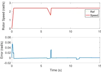
For the speed controller, the variable to be controlled is the generator rotor speed y = m, and the controller output is the q-axis
224
current reference u = iq*. Based on the first-order derivative of the rotor speed,
225 226 m 1.5 ψ ( m B m) p m q n T f i J J J (14) 227 228
the ADRC speed controller can be designed as follows. 229
1 1 2 0 1 2 2 0 1 * 0 2 0 ,0.5,0.01 , 0.25,0.01 ,0.3,0.01 / s m s s s s s s m m s s s q z z z b u fal z fal e u k fal e u u z b i (15) 231 232In (15), The constant b0s is set close to or equal to the constant b1.5npm/J as found in (14). It should be noted that the ADRC
233
speed controller does not need accurate plant model, which means that the unknown disturbances or variations of the mechanical 234
torque, friction coefficient, rotational speed, and the system inertia can be generalized as the total disturbance and estimated 235
inside the ESO of the ADRC. Due to the fact that the dynamics of the speed loop is much slower than the current loop and 236
considering a quite important system inertia for the studied 500 kW PMSG-based TST system (J4.359 10 kg m 4 2), the ESO
237
gains β1s, β2s should be much smaller than those of the current controller. The ESO and NLC gains of the ADRC speed controller
238
are tuned by simulation as 1s = 36, 2s = 3, k1s = 20.
239
C. Second-Order ADRC Control 240
There exists a possibility to merge the cascaded speed ADRC controller and the q-axis ADRC controller into one second-order 241
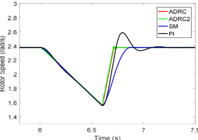
ADRC speed controller if the second-order derivation of the rotor speed is formulated as 242 243
T m q q m B m T s q e d d e m q k F v JL T f k F R i L i d J J JL (16) 244 245In (16), kT1.5 ψnp m is the PMSG torque constant; F is the total disturbance to be estimated and rejected by the second-order
246
ADRC; d represents unknown disturbances. Based on the basic structure of a order ADRC proposed in [15], the second-247
order speed controller for the PMSG-based TST can be designed as follows, 248 249
1 1 2 1 2 3 0 2 3 3 1 2 1 0 1 1 2 2 0 3 0 ,0.9,0.01 ,0.9,0.01 , , 0.5, 0.01 ,1.1,0.01 / s m s s s m m q z z z z z b u fal z fal e e e u k fal e k fal e u u z b v (17) 250 251 In (17), the constant b’0 can be set as kT/JLs; the derivative of the tracking error can be approximately calculated by (18),
252
with 1 = 0.001 and 2 = 0.0015, to avoid direct differentiation of the tracking error which may contain noises or sharp
253
variations; z1, z2, and z3 are the estimations of the rotor speed, its derivative and the total disturbance, respectively; ’1, ’2, and
254 ’
3 are the ESO gains and k’1 and k’2 are the NLC gains of the second-order ADRC controller.
255 256
2 1 2 1 1 2 1 1 1 1 1 e e s s (18) 257 258
Although the second-order ADRC speed controller enables to generate vq* directly from speed tracking error, this approach
259
involves a more complicated controller design and large gains have to be used in the ESO because the “total disturbance” needed 260
to be estimated by the second-order ADRC is greatly increased compared to the first-order one. 261
IV. SIMULATION AND COMPARATIVE STUDY 262
In this section, a 500kW direct-driven PMSG based TST (system parameters are listed in the Appendix) is studied. The 263
proposed cascaded ADRC approach will be compared with the second-order ADRC approach, the classical PI control approach, 264
and the hybrid speed sliding mode plus PI current control strategy. These four control strategies are shortened as ADRC, 265
ADRC2, PI and SM in the following comparison study. 266
A. Control Performance Evaluation under Disturbances of Current Velocity and Torque 267
In this part, the current velocity is considered as a constant value of 2m/s during 15s. A sudden current velocity fall (with -268
0.7m/s as the peak) is applied during 6 ~ 6.6s, and a large turbine torque thrust of 140kNm (equivalent to the nominal torque of 269
the PMSG) is added at 11~11.5s. 270
The speed performance of the ADRC approach during the entire 15s will be firstly illustrated and then comparisons with other 271
control methods will be carried out in different time periods. Figure 5 shows that the rotor speed response under the proposed 272
ADRC control strategy converges to the speed reference calculated by MPPT very rapidly. A rate limiter block is added at the 273
reference speed so that step speed changes can be avoided. Therefore, at the starting stage, the speed follows a slop reference. 274
During the tidal current disturbance and the turbine mechanical torque disturbance periods, the tracking error is about 0.03rad/s 275
and 0.01rad/s, which are lower than 1.3% of the steady-state speed of 2.377rad/s. 276
To compare the ADRC performance with other approaches, smaller time scales should be used. Figure 6 compares the rotor 277
speed response during the startup stage. It can be observed that the PI approach leads to an overshoot of 0.21rad/s, which is 8.8% 278
of the steady-state speed. The SM approach enables reducing the overshoot to 3% (0.08rad/s). ARDC has fastest convergent 279
speed with a negligible overshoot of 0.13%. ARDC2 presents no overshoot while it leads some small steady-state errors and 280
oscillations than the other approaches. 281 282 0 5 10 15 0 1 2 3 Ref Speed 0 5 10 15 Time (s) -0.02 0 0.02 0.04 0.06 0.08 283
Fig. 5. Generator rotor speed response with ADRC.
284 285
286
Fig. 6. Speed tracking comparison during starting stage.
287 288
Figure 7 shows that, under the current velocity drop disturbance, all the four control approaches are capable to follow a 289
dropping speed reference. However, when the disturbance is cleared at 6.6s, the speed reference has a quick rise to its steady-290
state value. In this case PI shows the biggest overshoot and longest settle time among other approaches. SM shows a smoother 291
and quicker convergent speed compared with PI; while ADRC and ADRC2 have the fastest convergent speed when the 292
disturbance is cleared. Although the speed performances of ADRC and ADRC2 are very similar, it should be noted that ADRC2 293
presents small fluctuations, which are caused by torque fluctuations due to the reason that ADRC2 has no q-axis current control 294
loop. 295
During the torque disturbance, the speed reference is not changed, which means that the ideal rotor speed should keep at the 296
steady-state value of 2.377rad/s. Figure 8 illustrates that the sudden rise of the turbine mechanical torque at 11s leads to a speed 297
rising and the clearance of the disturbance at 11.5s causes a speed dropping for PI and SM; while SM has less fluctuation and a 298
quick performance recovering than the PI approach. Both ADRC and ADRC2 achieve the smallest tracking error and no speed 299
drop error at the clearance of the disturbance at 11.5s. During the torque disturbance, ADRC has a maximum tracking error about 300
-0.007rad/s (as also shown in Fig. 5); ADRC2 seems to have even smaller error compared to ADRC, however speed fluctuations 301
can be seen with ADRC2. Figure 9 shows that ADRC2 leads to bigger torque fluctuations and this explains why speed 302
fluctuations exist in ADRC2. This reveals the drawback of ADRC2 due to the lack of a q-axis current control loop. 303
304
305
Fig. 7. Speed tracking comparison during current velocity disturbance.
306 307
308
Fig. 8. Speed tracking comparison during turbine torque disturbance.
309 310
311
Fig. 9. Generator torque during turbine torque disturbance.
312 313
In order to further investigate the control performance (speed tracking) of the above-evaluated strategies, two performance 314
indices ISE (Integral of the Square Error) and ITAE (Integral of the Time-weighted Absolute Error) are evaluated. They are 315 given by [31]. 316 317 2 1 2( ) t t ISE
e t dt (19) 318 2 1 1 ( ) ( ) t t ITAE
t t e t dt (20) 319In (19) and (20), e(t) is the speed tracking error; t1 and t2 represent the time-interval of the studied operating stages. The ISE
320
emphasizes on large overshoot or excessively underdamped behaviors. A small ISE value usually indicates a good capability of 321
large error suppression. The ITAE emphasizes on both initial response error and persistent errors. A low ITAE can therefore 322
reflect a satisfactory general error suppression performance during the duration of interest. ITAE has been also used to tune PID 323
controller parameters [32] or evaluate a controller performance [33]. In our case, both ISE and ITAE are calculated for the three 324
specific operating stages: starting stage (1s ~ 1.5s), current velocity disturbance stage (6s ~ 7.5s,) and torque disturbance stage 325
(11s ~ 12.5s). The achieved performance indices are listed in Table 1. 326
Based on the calculated performance indices, it has been found that for the starting stage, ADRC has the lowest ISE and ITAE 327
values, which demonstrate that it has a best error suppression capability. SM has a little higher ISE and ITAE values than PI for 328
the reason that a smooth response may lead to a lower error suppression speed in terms of error integration index. This result is 329
coherent with the simulation results shown in Fig. 6. During current velocity disturbance and torque disturbance stages, ADRC2 330
leads to the smallest ISE and ITAE values and ADRC has very similar results that are much smaller than those of SM and PI. It 331
should be also noted that during the disturbance stages, SM could have smaller ITAE values than PI. This means that nonlinear 332
controllers such ADRC and SM can have generally better disturbance rejection capabilities than constant parameters-PI ones. 333
Although ADRC2 seems slightly better than ADRC according to the index values during the disturbances stages, it should be 334
pointed out that ADRC2 suffers from the lack of a torque loop control (q-axis current loop) and therefore the resulted torque 335
fluctuations are slightly reflected in the speed tracking error due to the system inertia filtering effect. These observations show 336
that ISE and ITAE are interesting indices to evaluate a controller tracking performance. In this context, the speed tracking error 337
suppression capability of the proposed ADRC approach is well validated by these performance indices. 338
339
Table 1. Performance indices for three specific operating conditions.
340
Starting stage (1s ~ 1.5s)
Current velocity disturbance (6s ~ 7.5s) Torque disturbance (11s ~ 12.5s) ADRC ISE 0.00041 0.00009 0.000015 ITAE 0.00379 0.00296 0.00103 ADRC2 ISE 0.00103 0.00002 0.000003 ITAE 0.0278 0.00281 0.00069 SM ISE 0.0517 0.01536 0.0026 ITAE 0.0474 0.0378 0.012 PI ISE 0.015 0.00834 0.0011 ITAE 0.022 0.04 0.0073 341
B. Control Performance Evaluation under Swell Wave Disturbances 342
Swell waves are identified as the main cause of short-time power fluctuations in TST generation systems [6]. Figure 10 shows 343
the simulated marine current speed under swell effect (after 4s). Figure 11 illustrates the rotor speed response and its tracking 344
error by the proposed cascaded ADRC approach. It can be observed that the ADRC approach realizes a very good speed tracking 345
under swell-induced disturbances with negligible tracking errors. Figure 12 compares the energy production (calculated by the 346
integration of generator power) under swell disturbance by different control strategies studied in this work. At the end of the 347
simulation (60s), it can be observed that the energy yielding by PI control is about 2736Wh; SM and ADRC2 lead to a slightly 348
better energy yielding with 2737.5Wh and ADRC leads to a best yielding of 2738Wh. 349
350
351
Fig. 10. Marine current speed variations under swell effect.
353
Fig. 11. Generator speed tracking under swell disturbance with ADRC.
354 355
356
Fig. 12. Comparison of the energy productions.
357 358
V. ADRC UNDER SYSTEM PARAMETER VARIATIONS 359
When the generator resistance Rs and inductance Ls values are changed, the current-loop tracking performances are mainly
360
concerned. Figures 13 and 14 show the tracking errors of q-axis current under Rs variations (20% and 500%) and Ls variations
361
(50% and 200%). Large increase of resistance and inductance will cause current pulses, while the performances after 0.5s are 362
quite similar compared to the original parameter case. This illustrates the robustness of the ADRC current controller. 363
Figure 15 shows the speed responses under different system inertia. Smaller inertia will increase the speed-loop dynamics and 364
make the speed control easier. Larger system inertia requires higher torque to keep the speed rising rate. However, the q-axis 365
current, which directly contributes to the torque, is limited by 2 times of nominal current; and this explains the increased tracking 366
error at the starting stage in the 200% inertia case. ADRC works very well to converge the speed to the steady-state value rapidly 367
and results in no speed overshoot. 368
370
Fig. 13. Tracking error of the q-axis current under different stator resistance.
371 372
373
Fig. 14. Tracking error of the q-axis current under different stator inductance.
374 375
376
Fig. 15. Speed tracking error under different system inertia.
377
VI. CONCLUSIONS 378
In this paper, the cascaded ADRC approach was proposed to enhance the control performance of a PMSG-based tidal stream 379
turbine. An alternative, namely a second-order ADRC was also investigated. The ADRC strategy has clearly shown key features 380
such a lesser dependency on plant model analysis and efficient disturbance rejection capabilities. The carried out simulations and 381
the achieved results have clearly illustrated the effectiveness of the proposed ADRC strategy under various disturbance 382
conditions, while being compared to conventional PI and hybrid sliding mode/PI control strategies. This work has also shown 383
that the cascaded ADRC achieves better performance than the second-order ADRC in terms of smoothed torque. Performance 384
indices, namely ITAE and ISE, have been evaluated for three specific operating conditions. The achieved results have clearly 385
confirmed that the proposed ADRC approach outperforms the PI and hybrid sliding mode/PI control strategies. Robustness 386
against system parameter variations has also been investigated and verified for the cascaded ADRC approach. It has been 387
particularly shown that the proposed ADRC approach enables slightly improving a tidal stream turbine system energy production 388
during swell wave disturbance periods. 389
APPENDIX 390
TST System Parameters
391
Turbine blade radius 5.3m Maximum Cp value 0.41
Optimal tip speed ratio for MPPT 6.3 Rated marine current speed 3.0m/s Total system inertia 4.359 10 4kg.m2
System friction coefficient 0.0035 Generator nominal power 500kW Generator nominal torque 140kNm DC-bus rated voltage 1500V Rotor nominal speed 34.1rpm (3.57rad/s) Pole pair number 88 Permanent magnet flux 2.1435Wb Generator stator resistance 0.03Ω Generator d-q axis inductance 1.45mH
REFERENCES 392
[1] A.S. Bahaj, “Generating electricity from the oceans,” Renewable and Sustainable Energy Review, vol. 15, no. 7, pp.3399-3416, Sept.
393
2011.
394
[2] S. Benelghali, R. Balme, K. Le Saux, M. E. H. Benbouzid, J. F. Charpentier, and F. Hauville, “A simulation model for the evaluation of
395
the electrical power potential harnessed by a marine current turbine”, IEEE Journal of Oceanic Engineering, vol. 32, no. 4, pp.786-797,
396
Oct. 2007.
397
[3] Z. Zhou, M. E. H. Benbouzid, J. F. Charpentier, F. Scuiller, and T. Tang, “Developments in large marine current turbine technologies - A
398
review,” Renewable and Sustainable Energy Reviews, vol. 77, pp. 852-858, May 2017.
399
[4] H. Chen, T. Tang, N. Aït-Ahmed, M. E. H. Benbouzid, M. Machmoum, and M. E. Zaïm, “Attraction, challenge and current status of
400
marine current energy,” IEEE Access, vol. 6, pp. 12665-12685, 2018.
401
[5] K. Touimi, M. E .H. Benbouzid, and P. Tavner, “Tidal stream turbines: with or without a gearbox?,” Ocean Engineering, vol. 170, pp.
74-402
88, December 2018.
403
[6] Z. Zhou, F. Scuiller, J. F. Charpentier, M. E. H. Benbouzid, and T. Tang, “Power smoothing control in a grid-connected marine current
404
turbine system for compensating swell effect,” IEEE Transactions on Sustainable Energy, vol. 4, no. 3, pp. 816-826, July 2013.
405
[7] K. J. Åström and T. Hagglund, “The future of PID control,” Control Engineering Practice, vol. 9, no. 11, pp.1163-1175, Nov. 2001.
406
[8] V. Kumar, B. C. Nakra, and A. P. Mittal, “A review on classical and fuzzy PID controllers,” International Journal of Intelligent Control
407
and Systems, vol. 16, no. 3, pp.170-181, Sept./Dec. 2011.
408
[9] X. Duan, H. Deng, and H. Li, “A saturation-based tuning method for fuzzy PID controller,” IEEE Transactions on Industrial Electronics,
409
vol. 60, no. 11, pp. 5177-5185, Nov. 2013.
[10] A. Imura, T. Takahashi, M. Fujitsuna, T. Zanma, and M. Ishida, “Instantaneous-current control of PMSM using MPC: frequency analysis
411
based on sinusoidal correlation,” in Proceedings of the 2011 IEEE IECON, pp. 3551–3556, Melbourne (Australia), Nov. 2011.
412
[11] M. A. M. Cheema, J. E. Fletcher, D. Xiao, and M. F. Rahman, “A linear quadratic regulator-based optimal direct thrust force control of
413
linear permanent-magnet synchronous motor,” IEEE Transactions on Industrial Electronics, vol. 63, no. 5, pp. 2722–2733, May 2016.
414
[12] A. Levant, "Principles of 2-sliding mode design,” Automatica, vol. 43, no. 4, pp.576-586, April 2007.
415
[13] A. Levant, “Higher-order sliding modes, differentiation and output-feedback control," International journal of Control, vol. 76, no. 9-10,
416
pp.924-941, 2003.
417
[14] Z. Gao, Y. Huang, and J. Han, “An alternative paradigm for control system design,” in Proceedings of the 40th IEEE Conference on
418
Decision and Control, Orlando (USA), vol. 5, pp. 4578-4585, Dec. 2001.
419
[15] J. Han, “From PID to active disturbance rejection control,” IEEE Transactions on Industrial Electronics, vol. 56, n°3, pp. 900-906, March
420
2009.
421
[16] Y. Huang, W. Xue, Z. Gao, H. Sira-Ramirez, D. Wu and M. Sun, “Active disturbance rejection control: Methodology, practice and
422
analysis,” in Proceedings of the 33rd Chinese Control Conference, Nanjing (China), pp. 1-5, July 2014.
423
[17] Z. Gao, “Active disturbance rejection control from an enduring idea to an emerging technology,” in Proceedings of the 10th International
424
Workshop on Robot Motion and Control, pp. 269–281, Poznan (Poland), July 2015.
425
[18] S. Li, J. Yang, W. Chen, and X. Chen, “Generalized extended state observer based control for systems with mismatched uncertainties,”
426
IEEE Transactions on Industrial Electronics, vol. 59, no. 12, pp. 4792-4802, Dec. 2012.
427
[19] G. Wang, R. Liu, N. Zhao, D. Ding, and D. Xu, “Enhanced linear ADRC strategy for HF pulse voltage signal injection-based sensorless
428
IPMSM drives,” IEEE Transactions on Power Electronics, vol. 34, no. 1, pp. 514-525, Jan. 2019.
429
[20] B. Ahi and M. Haeri, "Linear active disturbance rejection control from the practical aspects," in IEEE/ASME Transactions on
430
Mechatronics, vol. 23, no. 6, pp. 2909-2919, Dec. 2018.
431
[21] J. Yang, W. Chen, S. Li, L. Guo, and Y. Yan, "Disturbance/uncertainty estimation and attenuation techniques in PMSM drives - a survey,"
432
in IEEE Transactions on Industrial Electronics, vol. 64, no. 4, pp. 3273-3285, April 2017.
433
[22] Y. Zuo, X. Zhu, L. Quan, C. Zhang, Y. Du, and Z. Xiang, “Active disturbance rejection controller for speed control of electrical drives
434
using phase-locking loop observer,” IEEE Transactions on Industrial Electronics, vol. 66, no. 3, pp. 1748-1759, March 2019.
435
[23] B. Guo, S. Bacha, and M. Alamir, "A review on ADRC based PMSM control designs," in Proceedings of the 2017 IEEE IECON, Beijing
436
(China), pp. 1747-1753, Oct. 2017.
437
[24] Z. Zhou, S. Ben Elghali, M. E. H. Benbouzid, Y. Amirat, E. Elbouchikhi, and G. Feld, “Control strategies for tidal stream turbine systems
438
– A Comparative Study of ADRC, PI, and high-order sliding mode controls,” in Proceedings of the 2019 IEEE IECON, Lisbon
439
(Portugal), pp. 6981-6986, Oct. 2019.
440
[25] T. Ane and L. Loron, “Easy and efficient tuning of PI controllers for electrical drives,” in Proceedings of the 2006 IEEE IECON, Paris
441
(France), pp. 5131-5136, Nov. 2006.
442
[26] Z. Zhou, “Modeling and power control of a marine current turbine system with energy storage devices,” PhD thesis, University of Brest
443
(France), 2014.
444
[27] S. Benelghali, M. E. H. Benbouzid, J. F. Charpentier, T. Ahmed-Ali, and I. Munteanu, “Experimental validation of a marine current
445
turbine simulator: application to a permanent magnet synchronous generator-based system second-order sliding mode control,” IEEE
446
Transactions on Industrial Electronics, vol. 58, n°1, pp. 118-126, Jan. 2011.
447
[28] D. Liang, J. Li, and R. Qu, “Sensorless control of permanent magnet synchronous machine based on second-order sliding-mode observer
448
with online resistance estimation,” IEEE Transactions on Industry Applications, vol. 53, n°4, pp. 3672-3682, July-Aug. 2017.
449
[29] D. H. Phan and S. Huang, “Super-twisting sliding mode control design for cascaded control system of PMSG wind turbine,” Journal of
450
Power Electronics, Vol. 15, No. 5, pp. 1358-1366, Sept. 2015.
451
[30] L. Fridman and A. Levant, “Higher order sliding modes,” Sliding Mode Control in Engineering, Chapter 3, pp.1-52, Marcel Dekker, New
452
York, 2002.
453
[31] W.S. Levine, “The control handbook," Section III, pp.169-173, CRC Press LLC, Florida, 1996.
[32] A. E. A. Awouda and R. B. Mamat, “Refine PID tuning rule using ITAE criteria,” in Proceedings of the 2010 IEEE ICCAE, Singapore,
455
pp. 171-176. Feb. 2010.
456
[33] P. Dahiya, P. Mukhija, A.R. Saxena, and Y. Arya, “Comparative performance investigation of optimal controller for AGC of electric
457
power generating systems,” Automatika, vol. 57, n°4, pp. 902-921, Dec. 2017.