On packing, colouring and identiﬁcation problems

(1)

HAL Id: tel-00801982

https://tel.archives-ouvertes.fr/tel-00801982

Submitted on 18 Mar 2013

HAL is a multi-disciplinary open access archive for the deposit and dissemination of sci-entific research documents, whether they are pub-lished or not. The documents may come from teaching and research institutions in France or abroad, or from public or private research centers.

L’archive ouverte pluridisciplinaire HAL, est destinée au dépôt et à la diffusion de documents scientifiques de niveau recherche, publiés ou non, émanant des établissements d’enseignement et de recherche français ou étrangers, des laboratoires publics ou privés.

On packing, colouring and identification problems

Petru Valicov

To cite this version:

Petru Valicov. On packing, colouring and identification problems. Data Structures and Algorithms [cs.DS]. Université Sciences et Technologies - Bordeaux I, 2012. English. �tel-00801982�

(2)

THÈSE

présentée à _LaBRI

L’UNIVERSITÉ BORDEAUX 1

École Doctorale de Mathématiques et Informatique de Bordeaux par

Petru VALICOV

pour obtenir le grade de

DOCTEUR

SPÉCIALITÉ Informatique

Problèmes de placement, de coloration et d’identification

Soutenue le 9 juillet 2012 au Laboratoire Bordelais de Recherche en Informatique Après avis des rapporteurs :

M. Frédéric Havet CR (HDR) INRIA Sophia-Antipolis

M. Yannis Manoussakis PR Université Paris-Sud

Devant la commission d’examen composée de :

M. Frédéric Havet CR (HDR) INRIA Sophia-Antipolis Rapporteur

M. Yannis Manoussakis PR Université Paris-Sud Rapporteur

M. Mickaël Montassier MdC (HDR) Université Bordeaux I Directeur

M. Arnaud Pêcher PR Université Bordeaux I Directeur

M. André Raspaud PR Université Bordeaux I Président

M. Éric Sopena PR Université Bordeaux I Directeur

M. Nicolas Trotignon CR (HDR) ENS Lyon Examinateur

Mme. Annegret Wagler MdC (HDR) Université Blaise-Pascal Examinatrice

(3)

(4)

-2012-Remerciements

Tout d’abord je tiens à remercier mes directeurs de thèse Arnaud, Mickaël et Éric. Merci Arnaud d’avoir encadré mon stage de M2 et d’avoir accepté d’encadrer ma thèse. Tu as supporté mon obstination pour le problème de placement et m’as laissé finaliser ce travail sans me pousser à faire autre chose. Tu m’as permis d’aborder les sujets que j’ai aimés, aussi différents qu’ils soient et tu m’as fait confiance durant ces trois années de thèse. Pour tout cela je te suis profondément reconnaissant.

Un grand merci à Mickaël de m’avoir aidé à colorier et à jouer avec les configurations réductibles. Merci également de m’avoir appris la rigueur même pour les preuves évidentes. L’attention avec laquelle tu lisais chaque fois mes notes m’a toujours surpris. J’espère main-tenant, après m’avoir montré tant de failles, être attentif moi aussi!

J’ai fait la connaissance d’Éric au premier semestre de mon M2 quand je faisais mes premiers pas dans la recherche. J’ai été impressionné (et je le suis toujours !) par ta gentillesse et ta facilité à aborder les problèmes même difficiles. Je suis très heureux d’avoir eu l’occasion d’enseigner avec toi à plusieurs reprises. Et pour tout cela je te remercie.

Je tiens à remercier Frédéric Havet et Yannis Manoussakis d’avoir accepté d’être rapporteurs de cette thèse et pour leurs remarques constructives sur le manuscrit. Merci également à Nicolas Trotignon et Annegret Wagler d’avoir fait partie de mon jury. Enfin je remercie André Raspaud d’avoir présidé le jury de thèse. André m’a enseigné la théorie de graphes durant mes deux années de master, sa rigueur et son enthousiasme durant ses cours m’ont marqué définitivement et m’ont donné une motivation de plus pour étudier les graphes.

Je remercie tous les autres collègues avec qui j’ai eu l’occasion de travailler : Aline Parreau, Cédric Joncour, Eleonora Guerrini, Florent Foucaud, Hervé Hocquard, Matjaž Kovše, Pascal Ochem, Reza Naserasr, Sylvain Gravier.

Ces trois années de recherche ont été faites au sein de l’équipe Graphes et Applications de CombAlgo. Je remercie tous les membres pour les séminaires organisés et les discussions qui ont dynamisé notre groupe. Merci à l’ANR IDEA et plus particulièrement à Ralf, de nous avoir donné l’occasion de travailler sur les codes identifiants sur plusieurs sites en France et d’avoir organisé BWIC 2011.

Tout au long de mon doctorat j’ai eu la grande chance d’enseigner à l’IUT Bordeaux 1 au sein d’une superbe équipe pédagogique. Un grand merci à tous ces membres!

Je souhaite remercier également le personnel administratif du LaBRI et notamment Philippe Biais, Brigitte Cudeville, Lebna Mizani, Cathy Roubineau de m’avoir aidé dans toutes les dé-marches administratives (pour les problèmes de visa tunisien par exemple...).

À mes co-bureaux, qui se sont succédé au fils de ces trois années, c’était super de bosser dans cette ambiance! Merci Abbas, Anasua, Dominik, Guillaume, Nicolas, Radu et Sri de m’avoir supporté. Je tiens particulièrement à remercier Sri de m’avoir soutenu et poussé à travailler sur la rédaction de ma thèse au moment où j’en avais perdu un peu la motivation.

Je n’oublie pas tous mes amis (qu’ils soient du LaBRI ou pas) : Aditya, Alizée, Anna, Anne-Claire, Brice, Edita, Eleonora, Eugen, Florent, Gaël, Hervé, Lorenzo, Mathieu, Reza, Sagnik, Sid, Svetlana R. et T., Youssouf.

Je remercie l’AFoDIB pour l’organisation des événements en dehors du cadre de travail. Merci

(5)

à tous les doctorants avec qui on s’est vraiment amusés pendant les séminaires, apéros-docs ou les journées sportives. Je pense à Adrien, Allyx, Anaïs, Clément, Émilie, Eve, Gabriel, Lorijn, Min, Pierre, Razanne, Thomas, Vincent... et j’en oublie certainement quelques-uns.

Enfin j’ai une petite pensée pour ma famille. Ils m’ont soutenu pendant toute la durée de mes études en Moldavie et en France. Mes parents, mes grands-parents (dont certains n’ont pas réussi à voir cette thèse finalisée), mon frère et ma sœur et leurs familles. Pour tout cela je vous témoigne une profonde reconnaissance. Mulţumesc pentru tot!

(6)

Problèmes de placement, de coloration et d’identification

Résumé : Dans cette thèse, nous nous intéressons à trois problèmes issus de l’informatique théorique, à savoir le placement de formes rectangulaires dans un conteneur (OPP), la coloration dite "forte" d’arêtes des graphes et les codes identifiants dans les graphes.

L’OPP consiste à décider si un ensemble d’items rectangulaires peut être placé sans chevauche-ment dans un conteneur rectangulaire et sans dépassechevauche-ment des bords de celui-ci. Une contrainte supplémentaire est prise en compte, à savoir l’interdiction de rotation des items. Le problème est NP-difficile même dans le cas où le conteneur et les formes sont des carrés. Nous présentons un algorithme de résolution efficace basé sur une caractérisation du problème par des graphes d’intervalles, proposée par Fekete et Schepers. L’algorithme est exact et utilise les MPQ-arbres - structures de données qui encodent ces graphes de manière compacte tout en capturant leurs propriétés remarquables. Nous montrons les résultats expérimentaux de notre approche en les comparant aux performances d’autres algorithmes existants.

L’étude de la coloration forte d’arêtes et des codes identifiants porte sur les aspects structurels et de calculabilité de ces deux problèmes. Dans le cas de la coloration forte d’arêtes nous nous intéressons plus particulièrement aux familles des graphes planaires et des graphes subcubiques. Nous montrons des bornes optimales pour l’indice chromatique fort χ0_sdes graphes subcubiques en fonction du degré moyen maximum et montrons que tout graphe planaire subcubique sans cycles induits de longueur 4 et 5 est coloriable avec neuf couleurs. Enfin nous confirmons la difficulté du problème de décision associé, en prouvant qu’il est NP-complet dans des sous-classes restreintes des graphes planaires subcubiques.

La troisième partie de la thèse est consacrée aux codes identifiants. Nous proposons une caractérisation des graphes identifiables dont la cardinalité du code identifiant minimum γID _est

n − 1, où n est l’ordre du graphe. Nous étudions la classe des graphes adjoints et nous prouvons

des bornes inférieures et supérieures serrées pour le paramètre γID _{dans cette classe. Finalement,} nous montrons qu’il existe un algorithme linéaire de calcul de γID _{dans la classe des graphes} adjoints L(G) où G a une largeur arborescente bornée par une constante. En revanche nous nous apercevons que le problème est NP-complet dans des sous-classes très restreintes des graphes parfaits.

Mots clefs : problème de placement orthogonal, graphes d’intervalles, MPQ-arbres, coloration forte d’arêtes, déchargement, graphes planaires, graphes parfaits, graphes adjoints, codes identi-fiants, complexité

Discipline : Informatique

LaBRI

Université Bordeaux 1 351 cours de la Libération, 33405 Talence Cedex (FRANCE)

(7)

On packing, colouring and identification problems

Abstract : In this thesis we study three theoretical computer science problems, namely the orthogonal packing problem (OPP for short), strong edge-colouring and identifying codes.

OPP consists in testing whether a set of rectangular items can be packed in a rectangular container without overlapping and without exceeding the borders of this container. An additional constraint is that the rotation of the items is not allowed. The problem is NP-hard even when the problem is reduced to packing squares in a square. We propose an exact algorithm for solving OPP efficiently using the characterization of the problem by interval graphs proposed by Fekete and Schepers. For this purpose we use some compact representation of interval graphs - MPQ-trees. We show experimental results of our approach by comparing them to the results of other algorithms known in the literature. We observe promising gains.

The study of strong edge-colouring and identifying codes is focused on the structural and computational aspects of these combinatorial problems. In the case of strong edge-colouring we are interested in the families of planar graphs and subcubic graphs. We show optimal upper bounds for the strong chromatic index χ0_s of subcubic graphs as a function of the maximum average degree. We also show that every planar subcubic graph without induced cycles of length 4 and 5 can be strong edge-coloured with at most nine colours. Finally, we confirm the difficulty of the problem by showing that it remains NP-complete even in some restricted classes of planar subcubic graphs.

For the subject of identifying codes we propose a characterization of non-trivial graphs having maximum identifying code number γID_{, that is n − 1, where n is the number of vertices. We study} the case of line graphs and prove lower and upper bounds for γID _{parameter in this class. At} last we investigate the complexity of the corresponding decision problem and show the existence of a linear algorithm for computing γID _{of the line graph L(G) where G has the size of the} tree-width bounded by a constant. On the other hand, we show that the identifying code problem is NP-complete in various subclasses of planar graphs.

Keywords : orthogonal packing problem, interval graphs, MPQ-trees, strong edge-colouring, discharging, planar graphs, perfect graphs, line graphs, identifying codes, complexity

Discipline : Computer Science

LaBRI

Université Bordeaux 1 351 cours de la Libération, 33405 Talence Cedex (FRANCE)

(8)

Introduction

1.1 Preliminaries . . . . 3

1.2 Some concepts on graphs . . . . 4

1.3 Some classes of graphs . . . . 5

1.4 Overview . . . . 7

In this chapter we begin with some standard definitions and notations. We follow up with common concepts and classes of graphs which will be used later on in this thesis. At the end of the chapter we present an overview of the problems considered.

1.1 Preliminaries

Graph A graph G = (V, E) is a set of elements V and a symmetric binary relation E defined on V . The elements of V are called vertices and the elements of E are called edges. To simplify notations, we will write V (G) (respectively E(G)) for the set of vertices (respectively edges) of a graph G. Two vertices u and v are adjacent if there exists an edge uv ∈ E. Two distinct edges uv and xy are adjacent if they share an endpoint (u = x for example). A graph is finite if the vertex set V is finite. A graph is simple if there can be at most one edge between every two vertices. Finally, a graph has a loop if there exists a vertex v ∈ V such that vv ∈ E, that is, v has an edge back to itself. In this document, unless specified, the graphs which are considered will be finite, simple and without loops.

Subgraph A subgraph of a graph G = (V, E) is a graph H = (V0, E0) such that V0 ⊆ V and

E0 ⊆ E(V0). If for every edge xy ∈ E(G) with x, y ∈ V0, xy ∈ E(H), then H is said to be the subgraph of G induced by V0 and is denoted G[V0].

Distance Two vertices u and v are at distance 1 if uv ∈ E. More generally, u and v are at distance k, if the length of a shortest path from u to v (the length being the number of edges) is k. For two vertices x and y of a graph G, distG(x, y) (or dist(x, y) if there is no ambiguity)

denotes the distance between x and y in G.

Neighbourhood, degree The adjacent vertices of a vertex v are also called neighbours of v. The open neighbourhood of a vertex v, denoted by N (v), is the set of vertices adjacent to v and the closed neighbourhood, denoted by N [v], is defined as the union N (v) ∪ {v}. Two vertices u and v are called twins in G if N [u] = N [v]. The number of vertices adjacent to a vertex v is the

degree of v, denoted by d_G(v) (d(v) if no ambiguity). We denote the maximum degree of a graph

G by ∆(G) (∆ if no ambiguity). A graph in which all vertices have the same degree k is said to

(11)

be k-regular. A class of graphs which we study in particular is the one of subcubic graphs which are graphs with maximum degree at most 3.

Connectivity A graph G is connected if for every pair of vertices u, v there exists a path between u and v in G. Otherwise the graph is said to be disconnected. A k-connected graph G is such that for every subset S of vertices with |S| = k − 1, G − S is connected.

Girth The girth of a graph is the length of one of its shortest cycles.

Cliques and stable sets A clique is a set of vertices which induces a complete graph that is a graph in which all vertices are pairwise adjacent. A clique of a graph G is a set of vertices of

G inducing a subgraph which is isomorphic to a complete graph. The clique number ω(G) is the

order of a maximum clique of G. In contrast, a stable or independent set of a graph G is a subset of pairwise non-adjacent vertices of G. Given an integer k ≥ 2, a subset I of vertices of G is called a k-independent set if for all distinct vertices x, y of I, dist_G(x, y) ≥ k. A 2-independent set is simply an independent set.

1.2 Some concepts on graphs

Operations on graphs

The complement of a graph G, denoted by G, is the graph whose vertex set is V (G) with two vertices being adjacent if and only if there is no edge between them in G.

Given a graph G, the k-th power Gk is the graph with vertex set V (G) such that two vertices are adjacent in Gk if and only if their distance in G is at most k.

We denote by G \ uv the graph obtained from G by removing the edge uv. Similarly, G − v denotes the graph obtained from G by removing vertex v from V (G) and all edges having v as an endpoint.

The join of two graphs, G₁ = (V₁, E1) and G2 = (V2, E2), denoted G1./ G2, is a graph whose vertex set is V1∪ V2 and its edge set is E1∪ E2∪ {v1v2 | v1∈ V1, v2∈ V2}.

Vertex and edge-colourings

A proper k-colouring of vertices of a graph G is a mapping from the vertex set to the set of integers {1, . . . , k} (called colours) such that two adjacent vertices have distinct colours. A graph is k-colourable if it admits a proper k-colouring. The chromatic number of G, denoted χ(G), is the smallest integer k such that G admits a k-colouring.

The notion of edge-colouring is defined similarly. A proper k-edge-colouring of a graph G is a mapping from the edge set to the set of integers {1, . . . , k} such that two adjacent edges have distinct colours. A graph is k-edge-colourable if it admits a proper k-edge-colouring. The

chromatic index of G, denoted χ0(G), is the smallest integer k such that G admits a proper

k-edge-colouring.

Dominating sets and Vertex covers

Given a graph G, a subset of vertices D ⊆ V (G) is called a dominating set if for every vertex

v ∈ V (G), D ∩ N [v] 6= ∅.

A vertex cover of a graph G is a subset of vertices C ⊆ V (G) such that for every edge

(12)

Matchings

A matching is a set of pairwise non-adjacent edges, and a perfect matching is a matching which covers all the vertices of the graph.

1.3 Some classes of graphs

In this section we recall some known families of graphs. We first fix the notations for the common classes of graphs that we will use throughout this manuscript.

We denote by C_n, P_n and K_n the cycle, path and complete graph on n vertices respectively.

Trees, Bipartite graphs

A tree is a connected graph with no cycle. In particular, the path Pn is a tree. A graph whose

connected components are trees is called a forest.

A bipartite graph is a graph G = (V, E) such that the vertex set is partitioned V = V1∪V˙ 2 such that V1 and V2 are independent sets. A complete bipartite graph Kn,m is a bipartite graph

with |V₁| = n and |V₂| = m such that ∀u ∈ V₁ and ∀v ∈ V₂, uv is an edge of this graph. In other words Kn,m contains the maximum possible number of edges.

It is an easy fact that forests are bipartite. For examples of such graphs see Figure 1.1.

V1

V2

(a) A general bipartite graph (b) A tree

Figure 1.1: Bipartite graphs

Planar graphs and Outerplanar graphs

A planar graph is a graph that can be drawn on the plane without edges crossing (see Fig-ure 1.2a for an example). A face of a planar graph G is the region bounded by the edges of G in a plane drawing of G. An outerplanar graph is a planar graph having a plane representation with all its vertices on the outer-face. An example is given in Figure 1.2b. Also, notice that the graph K4 (Figure 1.2a) is not outerplanar.

(a) A non-planar and a planar drawing of K4 (b) An outerplanar graph Figure 1.2: Examples of planar graphs and outerplanar graphs

(13)

Hypercubes

The hypercube of dimension d, denoted Hd, is a graph whose vertices are words of d bits such

that two vertices are adjacent if the corresponding words differ on a single bit, (equivalently one can say that the Hamming distance between these words must be equal to 1). The hypercube of dimension d can also be viewed as a union of two disjoint copies H0 and H1 of Hd−1, by adding

a new bit with value 0 (respectively 1) to the left of the words representing the vertices of H0 (respectively H₁) and by adding the edges between the corresponding vertices of two copies H₀ and H1. The hypercubes for the first three dimensions are shown in Figure 1.3.

0 1 00 01 10 11 000 001 010 011 100 101 110 111

Figure 1.3: Hypercubes H₁, H₂, H₃ respectively

Interval graphs

An interval graph is a graph G = (V, E) such that there is an assignment of intervals Iv

(v ∈ V ) of the real line to the vertices of G such that for every pair of vertices u and v, uv is an edge if and only if Iu∩ Iv 6= ∅. An example is shown in Figure 1.4. This class of graphs will

be the main topic of study in the second chapter of this manuscript, where we describe them in more details. 8 6 3 2 4 7 1 5 8 4 3 5 1 2 6 7

Figure 1.4: An example of interval graph

Split graphs, Chordal graphs

A graph G is a split graph if its set of vertices can be partitioned into two sets V1 and V2 such that V₁ is a clique and V₂ is an independent set.

A graph is chordal if it has no induced cycle of length k ≥ 4. In particular, interval graphs and split graphs are chordal.

Line graphs

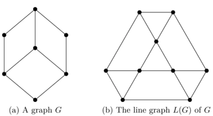
The line graph L(G) of a graph G is the graph with vertex set E(G), where two vertices of L(G) are adjacent if the corresponding edges are adjacent in G. We provide an example in Figure 1.5.

(14)

(a) A graph G (b) The line graph L(G) of G

Figure 1.5: An example of graph and its associated line graph

Perfect graphs

A graph G is perfect if for every induced subgraph H of G, χ(H) = ω(H). The perfect graphs which we mentioned in this section are bipartite graphs, interval graphs, split graphs and chordal graphs.

1.4 Overview

The three major subjects of this thesis are orthogonal packing, strong edge-colouring and

identifying codes. In this section we give a brief introduction to these topics. Further discussions

on the problems considered are developed in the corresponding chapters. We observe that the orthogonal packing problem can be formulated as a set-packing problem, whereas strong edge-colouring and identifying codes both have a natural formulation as a set covering problem.

The set packing problem (SPP for short) is defined as follows.

Definition 1.1. Let U be a set of m elements and S be a family of subsets of U . A packing P ⊆ S is a family of pairwise disjoint subsets P1, . . . , Pk. The set packing problem asks to find

P of largest cardinality (that is the maximum number of subsets P_i). In the weighted version of the problem, each set Pi has a positive weight w(Pi) and the goal is to find P of maximum total

weight.

The set cover problem (SCP for short) is defined as follows.

Definition 1.2. Let U be a set of m elements and S be a family of subsets of U . A cover C ⊆ S is a family of subsets C1, . . . , Ck such that U = C1∪ . . . ∪ Ck. The set cover problem is to find C

of smallest cardinality (that is the minimum number of subsets C_i). In the weighted version of the problem, each set Ci has a positive weight w(Ci) and the goal is to find C of minimum total

weight.

Set packing and set covering are two fundamental dual concepts in combinatorial optimization: each of them can be suitably transformed to the other. More precisely, let xS be a binary decision

variable such that

xS= 1 if subset S ⊂ S is selected, 0 otherwise

An integer linear programming formulation of the weighted set packing problem is:

max X S∈S w(S)xS subject to X S∈S: e∈S xS≤ 1, ∀e ∈ U xS∈ {0, 1}, ∀S ∈ S

(15)

where the constraint is that for every element e ∈ U there is at most one selected subset of S containing it.

The following dual formulation of the weighted set packing problem is an integer linear pro-gramming of the weighted set covering problem:

min X S∈S w(S)xS subject to X S∈S: e∈S xS≥ 1, ∀e ∈ U xS∈ {0, 1}, ∀S ∈ S

and the constraint is that for every element e ∈ U , at least one subset of S containing it must be selected.

The Orthogonal Packing Problem

Let V be a set of D-dimensional rectangular items and let C be a D-dimensional rectangular container. Let wd(v) ∈ Q+ and wd(C) be the length on dimension d of item v ∈ V and C

respectively. For a set of items S, we define w_d(S) =X

v∈S

wd(v).

The problem which we are interested in here in this manuscript, is defined as follows:

Definition 1.3. The D-dimensional orthogonal packing problem (OPP-D) is to decide if the set of items V fits into the container C without overlapping and with no rotation of the items. Formally speaking, we have to find out whether there exists a function f_d : V → Q+, ∀d ∈ {1, . . . , D}, corresponding to the position of the left corner of each of the items on dimension d, such that:

∀v ∈ V, fd(v) + wd(v) ≤ wd(C) (1.1)

∀v1, v2∈ V, (v1 6= v2), [fd(v1), fd(v1) + wd(v1)) ∩ [fd(v2), fd(v2) + wd(v2)) = ∅ (1.2) Constraint 1.1 is that item v must be packed without exceeding the width of C and Constraint 1.2 models the non-overlapping of the items.

OPP-D is a sub-problem of a well-known general problem whose objective in the base case is to minimize the total unused space:

Definition 1.4. Let V be a set of D-dimensional items and C a D-dimensional container. For each v ∈ V , let pv be an associated profit value. The D-dimensional orthogonal knapsack problem

(OKP-D) consists in selecting a subset V0 ⊆ V such that V0 is feasible and with maximum profit:

max V0_⊆V    X v∈V0 pv : V0 satisfies 1.1 and 1.2   

We focus on the two-dimensional case as it is the most studied one. However, our approach is general enough to be applied to the d-dimensional case, for any d ≥ 1.

We define the following binary decision variables:

ψiab=

(

1 if the coordinate (a, b) is covered by item i 0 otherwise

(16)

liab=

(

1 if the coordinate (a, b) is covered by the bottom left corner of item i 0 otherwise

A naive integer linear programming formulation of OKP uses space discretization ideas and can be seen as a set packing problem, which we provide below. By simplification, in the inequalities we ignore the containers’ boundary constraints:

maxX i X a X b piliab (1.3)

subject to ψ_i(a+j)(b+k)≥ l_iab, ∀i, 0 ≤ j ≤ w₁(i) − 1, 0 ≤ k ≤ w₂(i) − 1 (1.4) X i ψiab≤ 1, ∀a, ∀b (1.5) X a X b liab≤ 1, ∀i (1.6)

ψiab∈ {0, 1}, liab∈ {0, 1}, ∀i, a, b (1.7)

Constraint 1.4 ensures that a selected item i covering the coordinate (a, b) with its bottom left corner must cover all the coordinates (a + j, b + k), for 0 ≤ j ≤ w₁(i) − 1, 0 ≤ k ≤

w2(i) − 1. Constraint 1.5 is an overlapping constraint: there cannot be more than one item covering coordinate (a, b). Constraint 1.6 is to ensure that an item i is used only once.

The first formulation of the problem in the bidimensional case was given by Beasley in [9] and it uses a discretization technique similar to the one described above. Since then other authors provided similar approaches [26, 7, 16]. Other mathematical programming formulations exploit the information given by the placement of items relative to each other. For a deep survey of these approaches we refer to the PhD thesis of Joncour [63].

The main line of our research (described in Chapter 2) on this problem is based on a graph-theoretic model. Specifically, inspired by the characterization of packing solutions using interval graphs given by Fekete and Schepers in [39, 40] and by the competitive results based on this characterization [41], we propose an equivalent combinatorial formulation using MPQ-trees - a data structure which gives a compact representation of interval graphs, introduced in [68]. We describe an algorithm to enumerate the MPQ-trees under several constraints, in order to produce a solution to OPP-2.

Strong edge-colouring

Previously we defined proper colouring. We are interested in one variant of proper edge-colouring with an extra condition:

Definition 1.5. A strong edge-colouring of a graph G is a proper edge-colouring of G such that every two edges at distance exactly 2 are also assigned distinct colours. The strong chromatic

index of G, denoted χ0_s(G), is the smallest integer k such that G can be strong edge-coloured with

k colours.

Clearly, we have χ0_s(G) = χ(L(G)2), where χ is the classical chromatic number.

This observation gives rise to the following indirect but natural reformulation as an integer linear program of the strong edge-colouring problem

(17)

• Formulate χ(L(G)2_{) as the set covering problem with S as the set of all stable sets of L(G)}2_: minX S∈S xS subject to X S∈S:v∈S xS ≥ 1, ∀v ∈ V (L(G)2) xS ∈ {0, 1}, ∀S ∈ S S =nstable sets of L(G)2o

Up to our knowledge, the strong chromatic index has not been studied yet with the help of linear programming techniques.

Strong edge-colouring is closely related to another concept which gives a trivial lower bound for the strong chromatic index:

Definition 1.6. An antimatching is a set of edges such that no two edges are at distance strictly greater than 2. Denote by a(G), the size of the maximum antimatching of a graph G.

As in the case of strong edge-colouring, a(G) = ω(L(G)2). Obviously we have χ0_s(G) ≥ a(G). Definition 1.7. Let G = (V, E) be a graph. We define the closed neighbourhood of a clique Q, denoted N [Q], as the set of edges S, such that each edge of S has at least one end in Q. The maximal clique-neighbourhood is defined as:

ω_s0(G) = max {|N [Q]| , Q maximal clique of G} = max    X v∈V (Q) d(v) −|V (Q)| (|V (Q)| − 1) 2 , Q maximal clique of G   

It is easy to see that for any graph G, ω_s0(G) ≤ a(G) ≤ χ0_s(G). However, the inequalities can be strict: there are graphs such that ω0_s(G) < a(G) − λ, for a large value of λ. This is illustrated in Figure 1.6, where all the edges of the graph form an antimatching of size 3λ + 4 while ω_s0(G) = 2λ + 3. a c x1

· ··

xλ

··

·

λ 2

··

·

λ 2

Figure 1.6: A graph G such that ω0_s(G) < a(G) − λ

Proposition 1.8. If G is chordal, then χ0_s(G) = ω0_s(G).

Proposition 1.8 is an immediate consequence of the two following theorems proved in [17]: Theorem 1.9. (Cameron, 1989 [17]) If G is chordal, then L(G)2 is chordal.

(18)

Theorem 1.10. (Cameron, 1989 [17]) If G is chordal, then ω0_s(G) = a(G).

Since chordal graphs are perfect, for a chordal graph G we have ω_s0(G) = a(G) = ω(L(G)2) =

χ(L(G)2_{) = χ}0

s(G).

Lemma 1.11. If G has no induced C4 and C5, then a(G) = ωs0(G).

Proof. Let S be an antimatching of G and G[V (S)] be the graph induced by the endpoints of the

edges of S. By hypothesis of the lemma and by definition of an antimatching, G[V (S)] does not contain an induced cycle of length k ≥ 4. Therefore, G[V (S)] is chordal and, by Theorem 1.10,

ω_s0(G[V (S)]) = a(G[V (S)]).

Now, choose S of maximum size. We have: ω_s0(G[V (S)]) = |S| = a(G[V (S)]) = a(G). Moreover, ω0_s(G[V (S)]) ≤ ω_s0(G) and ω0_s(G) ≤ a(G). So, ω_s0(G) = a(G) as claimed.

A famous result of Grötschel, Lovász and Schrijver [56] states that the Lovász function ϑ(G) such that ω(G) ≤ ϑ(G) ≤ χ(G) can be computed in polynomial time. Hence we can derive the

following:

Remark 1.12. Let G be a graph such that χ0_s(G) = a(G). We have

χ0_s(G) = χ(L(G)2) = ϑ(L(G)2_{) = ω(L(G)}2_{) = a(G)}

Therefore, using the result of [56], χ0_s(G) can be computed in polynomial time by solving, in polynomial time, the linear program for the chromatic number.

The corresponding decision problem: given a graph G and an integer k, decide whether

χ0_s(G) ≤ k, is known to be NP-hard [78]. A natural question would be to know how "deep" is this hardness. That is to say, under which restrictions on graphs, the problem still remains NP-hard. Moreover, given this hardness result, a combinatorial point of view becomes all the more relevant: find polynomial-time computable lower and upper bounds for χ0_s on different classes of graphs. The main goal of Chapter 3 is to examine these two aspects: we show that strong edge-colouring remains NP-hard within very restricted subclasses of planar graphs; being motivated by several conjectures from the early 90’s, we also study the strong chromatic index on the family of subcubic graphs and outerplanar graphs.

Identifying codes

An identifying code of a graph G is a subset C of vertices of G such that ∀x ∈ V (G), N [x]∩C 6= ∅ (i.e. C is a dominating set) and ∀u, v ∈ V (G), N [u] ∩ C 6= N [v] ∩ C (i.e. C is a separating set) [66]. It is easy to see that a graph admits an identifying code if and only it has no twins.

One of the main questions is to find the size of a smallest identifying code of a graph G, denoted γID(G). Computing γID(G) is another instance of a set cover problem, which can be seen by the following reformulation:

Let GIDbe the identifying code hypergraph of G, where V (G) is the vertex set of GIDand there

are two kinds of hyperedges: the closed neighbourhood of each vertex of G and the symmetric difference of each pair of vertices of G. More formally, E(G_ID) = {N [v], N [u] N [v]|u, v ∈

V (G)}, where N [u] N [v] is the symmetric difference of N [u] and N [v]. It is then evident that

finding γID(G) is equivalent to computing the size of a minimum hitting set of G_ID, that is of a smallest subset of vertices covering all the hyperedges of G_ID. Therefore, we have the following

(19)

straightforward integer linear programming formulation: minX v∈V xv (1.8) subject to X v∈N [u] xv ≥ 1, ∀u ∈ V (1.9) X v∈N [u] N [w] xv ≥ 1, ∀u, w ∈ V, u 6= w (1.10) xu∈ {0, 1}n, ∀u ∈ V (1.11)

Here Constraints 1.9 and 1.10 are the domination and separation respectively.

Note that the identifying code problem was studied from the set cover perspective in [70]. Namely, it was proved by reduction from the set cover problem, that it is NP-hard to approximate

γID_{(G) within a factor of o(log(n)).}

It is known that for every twin-free graph G, except for K_n, γID_{(G) ≤ |V (G)|−1 [}₁₁_,₅₅_{]. Some} conjectures have been proposed for the classification of graphs achieving this extremal bound. In our work, disproving these conjectures, we give a full characterization of these graphs. We also improve lower and upper bounds for the identifying code number for the family of line graphs. Finally, we study the complexity of the problem by showing that it remains NP-hard in some restricted classes of perfect graphs.

In summary, in this manuscript we have considered three instances of integer linear program-ming problems. For each of them, we have tried to find better solutions by considering the additional information we get from the structure behind the problem. In the case of OPP, we introduce an algorithm that, in practice, works better than previously known algorithms. For the other two problems we considered (strong edge-colouring and identifying codes), on the one hand we improve previously known bounds, sometimes by considering restricted families of graphs such as planar graphs of high girth or line graphs. On the other hand, we show that finding the exact solution for these problems remains NP-hard even for such restricted families of graphs.

(20)

Orthogonal packing problem

Given a set of rectangular items of different sizes and a rectangular container, the aim of the two-dimensional Orthogonal Packing Problem (OPP-2), is to decide whether there exists a non-overlapping packing of the items in that container. The rotation of items is not allowed. This problem was proved to be NP-hard even in the restricted case, were a set of squares must be packed into a bigger square [73].

In this chapter, we present a new exact algorithm for solving OPP-2, detailed in Section 2.2.1. This procedure is based on the characterization of solutions using interval graphs proposed by Fekete and Schepers [39,40] and described in Section 2.1. The algorithm uses M P Q-trees as data structures, which were introduced by Korte and Möhring in [67,68] to recognize interval graphs. In Section 2.3 we establish the effectiveness of this algorithm on standard benchmarks. The main results we obtained and describe in this chapter are published in [65].

2.1 Formulation using interval graphs . . . . 14

2.2 MPQ-trees . . . . 16

2.2.1 Algorithm to check feasibility . . . 26

2.2.2 Symmetries and early unfeasibility detection . . . 27

2.3 Computational results and perspectives . . . . 31

Let V be a set of D-dimensional rectangular shapes. For d ∈ {1, . . . , D} and every v ∈ V , let w_d(v) ∈Q+ (resp. w_d(C)) be the length of v (resp. of the container C) with respect to the dimension d. For every subset of items S ⊆ V , let w_d(S) = X

v∈S wd(v). Let W (v) = D Y d=1 wd(v) and W (C) = D Y d=1

wd(C) be the volumes of the item v and of the container C respectively.

Formally OPP is defined as follows.

Definition 2.1. The D-dimensional orthogonal packing problem (OPP-D) is to decide if the set of items V fits into the container C without overlapping (if true, V is said to be feasible). Formally speaking, we have to find out whether ∀d ∈ {1, . . . , D} there exists a function f_d: V →Q+, such that:

∀v ∈ V, f_d(v) + w_d(v) ≤ w_d(C) (2.1) ∀v₁, v2 ∈ V, (v1 6= v2), [fd(v1), fd(v1) + wd(v1)) ∩ [fd(v2), fd(v2) + wd(v2)) = ∅ (2.2) where f_d(v) denotes the coordinate of the left corner of item v with respect to dimension d.

(21)

A natural generalization of the problem is the well-known orthogonal knapsack problem: Definition 2.2. Let V be a set of D-dimensional items and C a D-dimensional container. For each v ∈ V , let pv be an associated profit value. The D-dimensional orthogonal knapsack problem

(OKP-D) consists in selecting a subset V0 ⊆ V such that V0 _{is feasible and with maximum profit:}

max V0_⊆V    X v∈V0 pv : V0 satisfies 2.1 and 2.2   

A major step for solving the OPP, especially on hard instances, was made by Fekete and Schepers in late 90’s when they proposed to model the problem from a new graph-theoretic perspective. In the following section we explain their main idea as it is the basis of our approach.

2.1 Formulation using interval graphs

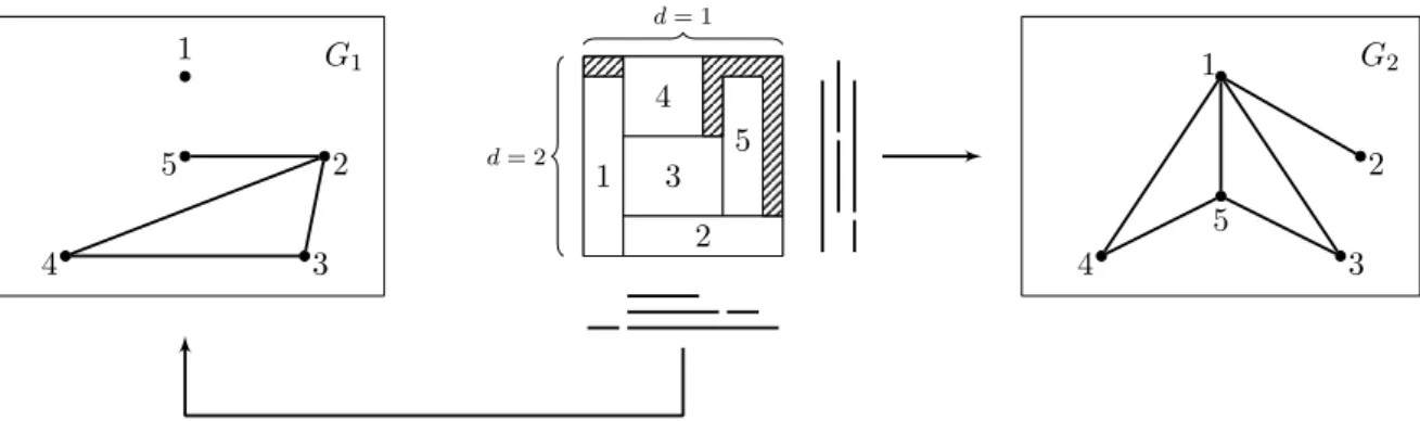
Fekete and Schepers [39,40] introduced a powerful characterization of feasible packings, based on interval graphs: given a feasible packing of a set of items V , for every dimension d, let

Gd= (V, Ed) be the interval graph with vertex set V and edge set Ed, such that ij is an edge if

and only if the projections of the packing of items i ∈ V and j ∈ V onto the dimension d intersect (see Fig. 2.1 for an illustration).

G1 1 2 3 4 5 d = 1 d = 2 4 1 3 5 2 G2 1 2 3 4 5

Figure 2.1: Example of 2D packing and its associated interval graphs

Hence every feasible packing induces a D-tuple of interval graphs which capture the relative positions of items. Fekete and Schepers established that the converse also holds:

Theorem 2.3 (Fekete and Schepers [39,40]). Given a D-dimensional container C, a set of items

V is feasible, if and only if there is a set of D graphs Gd = (V, Ed), with d ∈ {1, . . . , D}, such

that:

(P1) Every graph G_d is an interval graph;

(P2) For every stable set S of G_d, w_d(S) ≤ w_d(C); (P3)

D

\

d=1

Ed= ∅.

Definition 2.4. The D-tuple of graphs G_d satisfying the properties (P1), (P2) and (P3) of Theorem 2.3, is called a packing class.

Fekete, Schepers and van der Veen gave an efficient algorithm for solving OKP-D by solving its subproblem OPP-D [41]. The underlying idea of their algorithm is an exhaustive generation of tuples of interval graphs in order to find a packing class. To perform this generation efficiently, they used the following characterization of interval graphs:

(22)

Theorem 2.5 (Ghouilà-Houri [52], Gilmore and Hoffman [53]). Let a 2-chordless cycle be a cycle

v0, . . . , vn−1, v0 such that there is no edge vivj for i, j ∈ {0, . . . , n − 1} and |i − j| mod n = 2. A

graph G is an interval graph if and only if it contains no induced C₄ and its complement contains no 2-chordless cycle of odd length.

1 2 3 4 5 1 2 3 4 5 1 2 3 4 5

Figure 2.2: Symmetrical solutions in Fekete and Schepers’ model

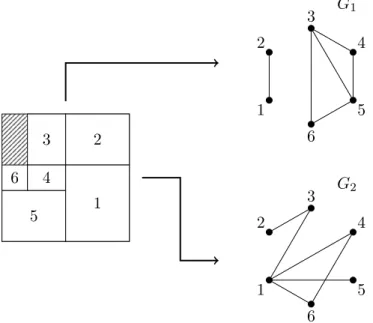
Despite its efficiency, their algorithm may enumerate symmetrical solutions. An example is given in Figure 2.2 where "almost" similar packing configurations are modeled by different pairs of interval graphs. Moreover, there are some degeneracy issues of Fekete and Schepers’ algorithm pointed out in [42], implying the generation of some unnecessary pairs of interval graphs. In Figure 2.3, we illustrate a packing configuration together with its associated interval graphs. These graphs are obtained with Fekete and Schepers’ algorithm and satisfy the properties of Theorem 2.3. However, there are some equivalent solutions which can be obtained by removing some edges in G1 or G2. For example, the edge between vertices 3 and 6 in G1 or between 1 and 3 in G₂ can be removed. 3 5 6 4 2 1 1 2 3 4 5 6 G2 1 2 3 4 5 6 G1

Figure 2.3: Degeneracy issues in Fekete and Schepers’ algorithm

To handle the issues mentioned above, Joncour and Pêcher [64] designed an algorithm based on some other characterization of interval graphs proposed by Fulkerson and Gross [50]. Before stating this characterization, we need the following definition.

Definition 2.6. Let G = (V, E) be a graph and Q₁, . . . , Qm its maximal cliques. A consecutive

arrangement of the maximal cliques of G is an order ≺ over the maximal cliques such that Qi ≺ Qj

if:

(23)

Theorem 2.7 (Fulkerson and Gross [50]). A graph G is an interval graph if and only if the maximal cliques of G can be linearly ordered to obtain a consecutive arrangement.

Definition 2.8. Let Q₁, . . . , Qm be the maximal (inclusionwise) cliques of a graph G. The

matrix M ∈ M_n,m({0, 1}) defined by M_ij = 1 if and only if vertex i belongs to clique Q_j is the

vertex/clique matrix of G. If there exists a consecutive arrangement of Q1, . . . , Qm, then on every

row of M , the 1’s occur consecutively and in this cases M is said to be a consecutive-ones matrix. In other words, one can consider a vertex/clique matrix M which is a 0-1 matrix were rows represent vertices, columns represent maximal cliques and M [i, j] = 1 if and only if vertex i belongs to clique j. Therefore, Theorem 2.7 states that a graph G is an interval graph if and only if M associated to G has the consecutive-ones property. The idea of the algorithm of Joncour and Pêcher was to generate consecutive ones matrices satisfying a condition equivalent to Property (P2) of Theorem 2.3. The main issue of this approach is that the same interval graph can be represented by several distinct vertex/clique matrices having the consecutive-ones property.

In the following section we detail our approach which uses a compact data-structure, designed to capture isomorphic interval graphs - MPQ-trees. These trees are an enriched representation of PQ-trees which were invented for testing the consecutive-ones property as well as graph pla-narity [15].

2.2 MPQ-trees

We start with main definitions and some useful results on MPQ-trees.

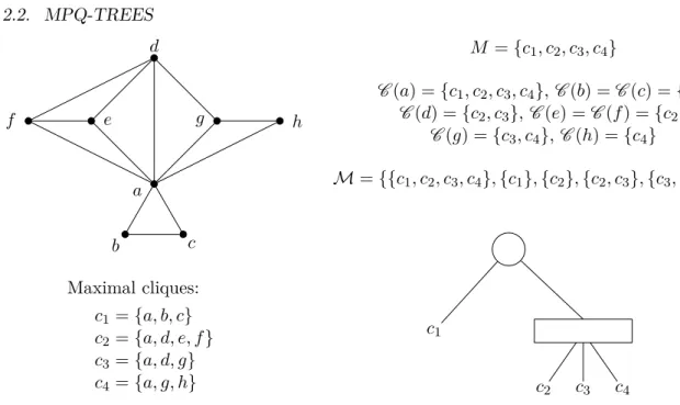
Let M be a set of elements and M a set of subsets of M . A PQ-tree is a data-structure representing all permutations of M in which the elements of each M0 ∈ M occur consecutively. It was introduced by Booth and Lueker in [14, 15]. In the case of an interval graph, M is the set of maximal cliques, and M is the set of allC (v), for every vertex v, where C (v) denotes the set of all maximal cliques containing vertex v. Namely, the constraints over M are designed to model the consecutive arrangement of the maximal cliques according to Theorem 2.7. For a better understanding we give an example in Figure 2.4. For the interval graph of this figure, there are four possible permutations of the maximal cliques such that in the representation of the associated vertex/clique matrix with the columns given by these orders, the 1’s occur consecutively:

              c1 c2 c3 c4 a 1 1 1 1 b 1 0 0 0 c 1 0 0 0 d 0 1 1 0 e 0 1 0 0 f 0 1 0 0 g 0 0 1 1 h 0 0 0 1                             c1 c4 c3 c2 1 1 1 1 1 0 0 0 1 0 0 0 0 0 1 1 0 0 0 1 0 0 0 1 0 1 1 0 0 1 0 0                             c2 c3 c4 c1 1 1 1 1 0 0 0 1 0 0 0 1 1 1 0 0 1 0 0 0 1 0 0 0 0 1 1 0 0 0 1 0                             c4 c3 c2 c1 1 1 1 1 0 0 0 1 0 0 0 1 0 1 1 0 0 0 1 0 0 0 1 0 1 1 0 0 1 0 0 0              

Before explaining the way how these permutations are captured by the PQ-tree illustrated on the figure, we provide few definitions from [14,15]:

Definition 2.9. A PQ-tree is a planar drawing of a rooted tree with two types of internal vertices: P and Q, represented by circles and rectangles respectively. The leaves of a PQ-tree are in one-to-one correspondence with the elements of M (the maximal cliques of an interval graph G). For an example see Figure 2.4. To avoid ambiguity between vertices of a graph and vertices of a PQ-tree, we call the latter ones nodes.

(24)

a b c d e f g _h Maximal cliques: c1= {a, b, c} c2= {a, d, e, f } c3= {a, d, g} c4= {a, g, h} M = {c1, c2, c3, c4} C (a) = {c1, c2, c3, c4},C (b) = C (c) = {c1} C (d) = {c2, c3}, C (e) = C (f) = {c2} C (g) = {c3, c4},C (h) = {c4} M = {{c₁, c2, c3, c4}, {c1}, {c2}, {c2, c3}, {c3, c4}, {c4}} c1 c2 c3 c4

Figure 2.4: An interval graph, its consecutive constraints and a PQ-tree representation.

The difference between P- and Q-nodes consists in the possible permutations of the reading orders of their sons:

Definition 2.10. The frontier F (T ) of a PQ-tree T , represents the permutation of the maximal cliques obtained by the ordering of the leaves of T from left to right. Two PQ-trees T and T0 are

equivalent, if one can be obtained from the other by applying the following rules a finite number

of times:

1. Arbitrarily permute the children of a P-node 2. Reverse the order of children of a Q-node

c1 c2 c3

c4 c5

c6 c7 c8 c8 c7 c6

c5 c4

c2 c3 c1

Figure 2.5: Equivalent PQ-trees

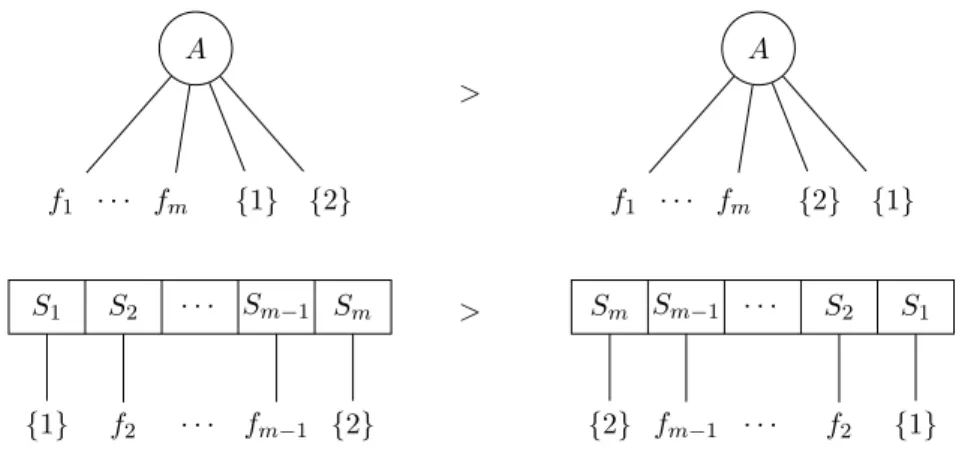
Figure 2.5 shows an example of two equivalent PQ-trees: the frontier of the right picture is obtained from the frontier of the left one, by reversing the order of the sons of both Q-nodes and by permuting the leaves c1, c2 and c3, sons of the P-node.

Now, let us come back to the PQ-tree of Figure 2.4. The main constraint over M of the corresponding interval graph is that the maximal cliques c₂, c₃ and c₄ can appear only in two possible orders c2, c3, c4 and the reversed order c4, c3, c2 (because of vertices d and g). Therefore, it can be easily checked that c₁, c₂and c₃must be sons of a Q-node as it is the only way to model exactly these two permutations.

A proper Ptree is a Ptree for which every P-node has at least two children and the Q-node has at least three children. From now on, by the term PQ-tree we will consider a proper PQ-tree.

(25)

An important result of Booth and Lueker is the following characterization of interval graphs using PQ-trees:

Theorem 2.11 (Booth and Lueker [14,15]). A graph G is an interval graph if and only if there exists a PQ-trees T such that F (T ) is a consecutive arrangement of the maximal cliques of G.

In the same articles, Booth and Lueker gave an algorithm recognizing interval graphs in linear time. The input of this algorithm is a graph G and it returns a PQ-tree associated to G if G is an interval graph and rejects the input otherwise. We do not describe their approach as in our algorithm for solving OPP-2 we use an extension of the notion of PQ-trees, introduced by Korte and Möhring in [67] for the same purpose of recognition of interval graphs. This extension allows to store more information about the vertices of the maximal cliques in the nodes of the tree and gives an easier method of recognizing interval graphs than the method using classical PQ-trees proposed by Booth and Lueker. We provide its definition below:

Definition 2.12. A modified PQ-tree (MPQ-tree for short) associated with a graph G is an extension of a PQ-tree where the nodes of the tree are labelled with some subsets of vertices of

G, such that each branch of the MPQ-tree represents a maximal clique. A P-node is assigned

only one set, while a Q-node is assigned a set for each of its children. Here are the rules of the labelling:

• A P-node is labelled by the set of vertices of G which are only contained in all cliques represented by the subtree of T rooted in this node.

• A leaf is labelled by the set of vertices of G contained only in the clique represented by this leaf.

• A Q-node, with m children F₁, . . . , Fm, is labelled by a list of sets Sk, for k ∈ {1, . . . , m},

each of them being called a section such that a section S_k corresponds to the child F_k in the left-to-right order. Each section Sk(k ∈ {1, . . . , m}) is a subset Sk of vertices of G such

that S_k is contained in all cliques represented by the subtree rooted in F_k. Additionally, every vertex of S_k must belong to all cliques represented by the subtree rooted in some other child of the Q-node, say Fl, where l ∈ {1, . . . , m} and l 6= k.

a b c d e f g _h {a} {b, c} {d} {d, g} {g} {e, f } ∅ {h}

Maximal cliques: c1= {a, b, c} c2 = {a, d, e, f } c3= {a, d, g} c4 = {a, g, h} Figure 2.6: The interval graph of Figure 2.4 and an MPQ-tree representation.

We will say that a node N of an MPQ-tree associated with a graph G contains a vertex v of

G if v ∈ VN, where VN is the vertex set or section (in case of a Q-node) of the label of N . Notice

that from the definition of an MPQ-tree, a vertex v of G is contained in exactly one MPQ-tree node. However, v can be contained in more than one section of a Q-node. Figure 2.6 gives an illustration of an MPQ-tree based on the interval graph of Figure 2.4. Observe that the structure

(26)

of both the PQ-tree of Figure 2.4 and the MPQ-tree of Figure 2.6 are the same, only the labels of the nodes are different, the branches of the MPQ-tree being the maximal cliques.

Figure 2.7 shows an example of an MPQ-tree associated with an interval graph G, where both representations model the intersections in dimension 1 of a feasible packing in terms of maximal cliques (the intersections are given by the strips in the picture).

2 3 5 4 6 7 8 1 {2} {2, 5} {5, 7} {7} {1} ∅ {3, 4} {6} ∅ {8} Maximal cliques: {1, 2}, {2, 3, 4, 5}, {2, 5, 6}, {5, 7}, {7, 8} 2 ₇ 1 5 8 3 6 4 7

Figure 2.7: An interval graph, an associated MPQ-tree and the packing configuration Similarly as in the case of PQ-trees, Korte and Möhring established the connection between MPQ-trees and interval graphs by proving the following characterization of interval graphs: Theorem 2.13 (Korte and Möhring [67,68]). A graph G is an interval graph if and only if there exists an MPQ-tree associated with G.

Therefore, we may consider MPQ-trees instead of interval graphs as Theorem 2.13 gives an equivalence between the two structures. The following lemma is crucial for our algorithm since it is the basis for an incremental generation of MPQ-trees.

Lemma 2.14 (Korte and Möhring [68]). Let G be an interval graph and T its associated MPQ-tree. Then G + u (where u is a vertex added to G) is an interval graph if and only if the following holds:

1. All vertices adjacent to u are contained in a unique path of T .

2. For each Q-node N , labelled with sections S1, . . . , Sm, let S = S1∪. . .∪Sm. Then S ∩N (u) ⊆

S1 or S ∩ N (u) ⊆ Sm

In other words, Lemma 2.14 says that while building an MPQ-tree incrementally from an interval graph (i.e. adding vertices of the graph one by one) only one path of this tree must be updated and due to the properties of the reading orders of children of nodes of an MPQ-tree, this path can be chosen to be the leftmost one. This restricts considerably the number of cases to consider while updating the MPQ-tree.

To describe the idea of Korte and Möhring’s algorithm for the recognition of interval graphs, an idea which is reused in our approach, we first need to provide the following definition:

Definition 2.15. Given a graph G, a simplicial elimination scheme (also called a perfect vertex elimination scheme) is an ordering σ = [v₁, . . . , vn] of the vertices of G such that the graph induced

by the vertices of N (vi) ∩ {vi+1, . . . , vn} is a clique.

An important fact is that a graph is a chordal graph if there exists a simplicial elimination

scheme for the vertices of this graphs [33,50,87]. Therefore, interval graphs being chordal must admit one too.

(27)

A simplicial elimination scheme for the vertices of a graph G can be obtained by running a

LexBFS algorithm on G (introduced in [88]). In particular, if a graph is chordal, then a LexBFS algorithm produces an order of the vertices σ = [v₁, . . . , vn], such that [vn, vn−1, . . . , v1] is a simplicial elimination scheme.

Using Theorem 2.13 and Lemma 2.14, Korte and Möhring gave a much simpler linear algo-rithm than the one of Booth and Lueker, recognizing interval graphs, by building iteratively an associated MPQ-tree [68]. Their algorithm uses a LexBFS-ordering of the vertices of the input graph to iteratively build a corresponding MPQ-tree. Let G = (V, E) be an interval graph with an associated MPQ-tree T_G and u the vertex to be inserted in T_G to obtain the MPQ-tree T_G+u associated with the graph G + u. Since vertices are inserted in LexBFS-order, N (u) must induce a clique. Let N be a node of T_G. If N is of type P or a leaf, then let V_N be its associated vertex set and if N is a Q-node, let V_N be the vertex set corresponding to the first section. The principle of Korte and Möhring’s algorithm is the following:

• Find the unique path P of the current MPQ-tree having a node N such that VN∩ N (u) 6= ∅.

This path can be either leftmost or rightmost.

• Find the first node N∗ in the bottom-up traversal such that ∃j ∈ VN∗, j ∈ N (u).

• Select the corresponding pattern and apply the suitable replacement: let VN∗ = A ∪ B be the partition of VN∗ such that A = VN∗∩N (u) and B = VN∗\A. Let N

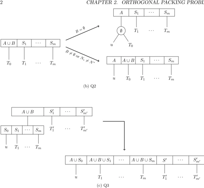
∗_{be the highest node} in P such that V_N∗\ N (u) 6= ∅ if it exists and let N∗= N_∗ otherwise. Due to Lemma 2.14, the patterns which can be applied are described in Figures 2.8, 2.9 and 2.10. In the case when N∗ 6= N∗ the patterns are applied recursively by rewriting the current tree starting from N∗ up to N∗, to obtain a valid MPQ-tree. We omit details which are rather technical. For an elaborate explanation, see the original paper [68]. We just strengthen the fact that the process is deterministic e.g. at each step only one pattern can apply. If no pattern can be applied to the current configuration, then G + u is not an interval graph.

[A ∪ B] B =∅ [A ∪ u] B 6= ∅ A u B [A ∪ B] N∗6= N ∗ A A u B

Figure 2.8: Templates for a leaf: VN∗= A ∪ B

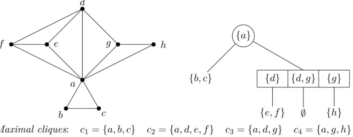
For an example of construction of an MPQ-tree from an interval graph using Korte and Möhring’s templates, we illustrate the successive application of patterns in Figure 2.11. The LexBFS order applied in the figure is σ = [8, 7, 5, 6, 2, 3, 4, 1]. The building of the MPQ-tree is done in eight step (from s1 to s8 in the picture), provided the default operation in the very first step s0: an empty MPQ-tree T is created and vertex 8 is inserted in T as a leaf. Below, we give a detailed explanation of which of the templates of Figures 2.8, 2.9, 2.10 is applied in each of the steps together with the value of each of the parameters VN∗, B:

• s1: a leaf template of Figure 2.8 with VN∗ = {8}, B = ∅, N∗= N ∗_; • s2: a leaf template of Figure 2.8 with VN∗ = {7, 8}, B 6= ∅, N∗ = N

∗_;

• s3: since vertex 6 is not adjacent to vertex 7, N∗ _{is the root P-node with V}

N∗ = {7} and hence N∗ 6= N∗. Therefore, the leaf template of Figure 2.8 with VN∗ = {5}, N∗ 6= N

∗ _is applied. In the following step the higher nodes of the tree must be changed in order to obtain N∗ = N∗;

(28)

A ∪ B T1 · · · Tm B= ∅ A u T1· · · Tm B 6= ∅ A u B T1· · · Tm A ∪ B T1 · · · Tm N∗6= N∗ A A u B T1 · · · Tm (a) P1 and P2: VN∗= A ∪ B A ∪ B S0 S1 · · · Sm0 u T₁0 · · · T0 m0 T1 · · · Tm A ∪ S₀ A ∪ B ∪ S₁ · · · A ∪ B ∪ S_m0 _{A ∪ B} T₁0 · · · T_m00 u ∅ T1 · · · Tm (b) P3: VN∗= {u} and N∗6= N ∗

Figure 2.9: Templates for a P-node

A ∪ B1 · · · A ∪ Bm T1 · · · Tm N∗= N∗ A u B1 · · · Bm T1 · · · Tm N_∗ 6=_N ∗ A A u B1 · · · Bm T1 · · · Tm (a) Q1

(29)

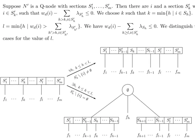
A ∪ B S1 · · · Sm T0 T1 · · · Tm B= ∅ A S1 · · · Sm ∅ u T0 T1 · · · Tm B 6= ∅ or_N ∗6=_N ∗ A A ∪ B S1 · · · Sm u T0 T1 · · · Tm (b) Q2 A ∪ B S0₁ · · · S_m0 0 S0 S1 · · · Sm u T1 · · · Tm T₁0 · · · T_m00 A ∪ S₀ A ∪ B ∪ S₁ · · · A ∪ B ∪ Sm S0 · · · S0m0 u T1 · · · Tm T10 · · · Tm00 (c) Q3

Figure 2.10: Templates for a Q-node

• s4: the P-node template P3 of Figure 2.9b with VN∗ = {5}, N∗ 6= N

∗_{, B 6= ∅ is applied and} at the end we obtain N ∗ = N∗;

• s5: a leaf template of Figure 2.8 V_N_∗ = {6}, B = ∅, N∗ = N∗; • s6: a leaf template of Figure 2.8 V_N_∗ = {2, 6}, B 6= ∅, N∗ = N∗; • s7: a leaf template of Figure 2.8 V_N_∗ = {3}, B = ∅, N∗ = N∗;

• s8: a leaf template of Figure 2.8 V_N_∗ = {3, 4}, N∗ 6= N∗, then the higher nodes of the tree must be changed in order to obtain N∗ = N∗;

• s9: the Q-node template Q3 of Figure 2.10c is applied.

The order σ is not the only LexBFS order possible. For instance, one could start building from vertex 1, in which case the obtained MPQ-tree would be the equivalent of the one of Figure 2.11 (with the reading order from right to left).

In order to formulate Property (P2) of Theorem 2.3 with respect to MPQ-trees we define the width of the nodes:

Definition 2.16. For every node N of an MPQ-tree associated with a dimension d of a packing configuration, the width λ_N ∈Q+ _{of N is as described below:}

(30)

{8} s1 {7, 8} s2 {7} {5} {8} s3 {7} {5} {5} {6} ∅ {8} s4 {5} {5, 7} {7} {6} ∅ {8} s5 {5} {5, 7} {7} {2, 6} ∅ {8} s6 {5} {5, 7} {7} {2} {3} {6} ∅ {8} s7 {5} {5, 7} {7} {2} {3, 4} {6} ∅ {8} s8 {5} {5, 7} {7} {2} {2} {1} ∅ {3, 4} {6} ∅ {8} s9 {2} {2, 5} {5, 7} {7} {1} ∅ {3, 4} {6} ∅ {8}

Figure 2.11: Building the MPQ-tree of Figure 2.7 with the templates from [68]

• If N is a leaf L labelled with the set VL, then λL = max i∈VL

{wd(i)} if VL 6= ∅ and λL = 0

otherwise.

• If N is a P-node P labelled with the set V_P, and λ_f₁, . . . , λfm are the widths of each of its

children, then λP = max    m X j=1 λfj, max i∈VP {w_d(i)}   

• If N is a Q-node Q, let S1, . . . , Sm be its sections and λf1, . . . , λfm the widths of each of

the children of the node. In order to define the width λ_Q, we first define, recursively from

m to 1, the widths of its sections: λSj, ∀1 ≤ j ≤ m:

λSm = λfm

Suppose λ_S_k+1, . . . , λSm are defined, then

λSk = max    λfk, max i∈Sk,i /∈Sk−1    wd(i) − X h>k, i∈Sh λSh      

(31)

The width of N is given by the following formula λQ= m X k=1 λSk

It follows from definition that for every node N with children f₁, . . . , fm, λN ≥ m

X

k=1

λfk.

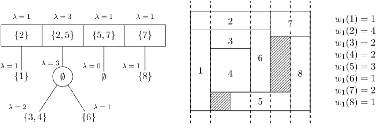
In Figure 2.12 we illustrate the notion of widths on the MPQ-tree and the corresponding packing configuration from Figure 2.7. The sizes of the items in dimension 1 are given in the right part of the picture.

{2} λ = 1 {2, 5} λ = 3 {5, 7} λ = 1 {7} λ = 1 {1} λ = 1 ∅ λ = 3 {3, 4} λ = 2 {6} λ = 1 ∅ λ = 0 {8} λ = 1 2 ₇ 1 5 8 3 6 4 7 w1(1) = 1 w1(2) = 4 w1(3) = 2 w1(4) = 2 w1(5) = 3 w1(6) = 1 w1(7) = 2 w1(8) = 1

Figure 2.12: An MPQ-tree with the widths of its nodes and a corresponding packing We now establish the inequality relation between the width of an item and the width of the MPQ-tree node containing this item:

Lemma 2.17. Let G_d = (V, E_d) be an interval graph of a packing class and T_d an associated MPQ-tree. Let v be an item of V . For every P-node or leaf N such that v belongs to the label of

N , we have wd(v) ≤ λN. For every Q-node N containing v in the labels of some of its sections,

we have w_d(v) ≤

l

X

h=k

λSh, where Sk, . . . , Sl are the sections of N containing v.

Proof. The cases of a P-node and of a leaf are obvious. Suppose N is a Q-node with sections S1, . . . , Sm and children f1, . . . , fm. Since branches associated with sections Sk, . . . , Sl of N are

all the cliques containing v, we have λSk ≥ wd(v) −

l X h=k+1 λSh. Hence, wd(v) ≤ l X h=k λSh.

The following proposition translates Property (P2) of Theorem 2.3 in terms of widths of the MPQ-tree nodes, the previous lemma being helpful to prove the converse part of the equivalence. Proposition 2.18. Let G be an interval graph. The graph G satisfies Property (P2) if and only if for every associated MPQ-tree T of G, the width λ_R of the root of T verifies λ_R≤ w_d(C).

Proof.

Suppose G satisfies Property (P2) and consider an MPQ-tree T of G with root R. We will prove that λR≤ wd(C).

The proof is by induction on the distance between R and the nodes of T . Let H(k) be the assertion: ”If N is a node of T at distance k from R, then there is a stable set S of G[N ] such that λ_N ≤ w_d(S), where G[N ] is the subgraph of G induced by the set of vertices of G contained in the labels of the subtree of T rooted in N .”