HAL Id: tel-01951540
https://tel.archives-ouvertes.fr/tel-01951540
Submitted on 11 Dec 2018
HAL is a multi-disciplinary open access
archive for the deposit and dissemination of sci-entific research documents, whether they are pub-lished or not. The documents may come from teaching and research institutions in France or abroad, or from public or private research centers.
L’archive ouverte pluridisciplinaire HAL, est destinée au dépôt et à la diffusion de documents scientifiques de niveau recherche, publiés ou non, émanant des établissements d’enseignement et de recherche français ou étrangers, des laboratoires publics ou privés.
Pranav Chandramouli
To cite this version:
Pranav Chandramouli. Turbulent complex flows reconstruction via data assimilation in large eddy models. Fluids mechanics [physics.class-ph]. Université Rennes 1, 2018. English. �NNT : 2018REN1S035�. �tel-01951540�
For my parents, who got me here and to Palak, who got me through
Acknowledgements
Etienne and Dominique, your guidance has ensured I traverse successfully the narrow, treacherous straits that is a PhD program. Your rigorous standards, academic familiarity and attitude towards research are traits I hope to inculcate and emulate. I would like to express my profound thanks to you for taking me in this program, and for guiding me, constantly, through it.
To Sylvain, without whom I would not be here, I am thankful for your guidance in everything numerical.
To my friends, past and present, in the corridor - ‘Vincent, Benoit, Sandeep, Anca, Antoine, Manu, Valentin, and countless others’, I thank you for all the special memories, fun and funny, we had over the past three years. Special mention to Long, for our mutual fifa addiction, Carlo, for our coffee, and Yacine, for our multitude of breaks. A big thank you to Huguette for taking care of all the administrative works that I would have, otherwise, been swamped with.
A final thanks to my family whose constant support and never-ending belief in me always motivated me to work harder and do something more.
Introduction en français ix
Introduction xv
1 Fluid flow fundamentals 1
1.1 Computational fluid dynamics . . . 2
1.1.1 A brief history of CFD . . . 2
1.1.2 Governing equations . . . 2
1.1.3 Discretisation techniques . . . 3
1.1.4 Boundary conditions . . . 5
1.1.5 Turbulence modelling . . . 6
1.2 Experimental fluid dynamics . . . 6
1.2.1 A brief history of EFD . . . 6
1.2.2 Hot wire anemometry (HWA) . . . 7
1.2.3 Laser doppler anemometry (LDA) . . . 7
1.2.4 Particle image velocimetry (PIV) . . . 8
1.3 Limitations . . . 10
1.4 Coupling EFD and CFD . . . 11
2 Turbulence modelling 15 2.1 Reynolds averaged Navier-Stokes . . . 17
2.1.1 RANS equations . . . 17
2.1.2 Turbulent-viscosity models . . . 18
2.1.3 Reynolds stress models (RSM) . . . 21
2.2 Large eddy simulation . . . 21
2.2.1 Filtered Navier-Stokes equations . . . 22
2.2.2 Smagorinsky models . . . 23
2.2.3 WALE model . . . 27
2.2.4 Models under location uncertainty . . . 28
2.2.5 Other Approaches . . . 32
2.3 Hybrid approaches . . . 34
3 Large eddy simulation - applications 37 3.1 Flow solver - Incompact3d . . . 37
3.2 Channel flow at Re⌧ = 395 . . . 45
3.2.1 Channel flow parameters . . . 45
3.2.2 Channel flow results . . . 46
3.3 Wake flow around a circular cylinder at Re = 3900 . . . 49
3.3.1 Introduction to wake flow . . . 49 v
3.3.2 Flow configuration and numerical methods . . . 53
3.3.3 Wake flow results . . . 56
3.4 Concluding remarks . . . 76
4 Stochastic Simulations - vortex forces and Langmuir circulation 79 4.1 Introduction . . . 79
4.2 Mathematical formulations . . . 80
4.2.1 CL model . . . 80
4.2.2 Large-scale drift MULU . . . 80
4.3 Vortex force theory for streak formation . . . 83
4.4 Large-scale application . . . 88
5 Data assimilation techniques 93 5.1 Mathematical Formulation . . . 94
5.2 Data assimilation - a review . . . 94
5.3 4D-Var approach . . . 98
5.3.1 4D-Var Algorithm Variants . . . 100
6 Flow reconstruction - snapshot optimisation method 105 6.1 Introduction . . . 105
6.2 Snapshot optimisation method . . . 107
6.2.1 SO model concept . . . 107
6.2.2 Mathematical formulation . . . 108
6.2.3 Reduced order formulation . . . 110
6.2.4 Averaging SO method . . . 111
6.3 Application and results . . . 111
6.3.1 Synthetic case-studies . . . 112
6.3.2 Algorithm Enhancement Techniques . . . 117
6.3.3 Experimental case-studies . . . 120
6.4 Conclusion . . . 127
7 Data assimilation - wake flow at Re = 3900 129 7.1 Code Formulation . . . 129 7.1.1 4D-Var . . . 129 7.1.2 4D-Varles . . . 136 7.2 3D synthetic assimilation . . . 142 7.2.1 Flow configuration . . . 142 7.2.2 Observations construction . . . 144
7.2.3 Initial background construction . . . 146
7.2.4 Results and Discussion . . . 146
7.3 2D synthetic assimilation . . . 152
7.3.1 Flow configuration . . . 152
7.3.2 Observations construction . . . 152
7.3.3 Initial background construction . . . 156
7.3.4 Results and Discussion . . . 156
7.4 Background covariance . . . 162
7.5 Coefficient estimation . . . 165
7.6 Combined case study . . . 168
Contexte
L’étude des fluides remonte à l’antiquité aux travaux d’Archimède tels que le fameux ‘principe d’Archimède’ sur la flottabilité. Au fil du temps, le domaine s’est diversifié dans l’étude des fluides stationnaires (ou de la statique des fluides) et des écoulement fluides (ou de la dynamique des fluides). La dynamique des fluides peut être subdivisée en l’étude de fluides newtoniens et non-newtoniens en fonction de la forme de la contrainte de frottement moléculaire. Les fluides newtoniens, qui sont les fluides étudiés dans cette thèse, ont un taux de déformation proportionnel à la contrainte appliquée et leur dynamique s’exprime mathématiquement au moyen des équations de conservation de la masse, de quantité de mouvement et d’énergie. L’étude de la mécanique des fluides a été la pierre angulaire de nombreuses avancées dans le domaine de l’aérospatial, de la prévision météorologique, des applications géophysiques, de l’automobile, du génie civil, etc. Des approches plus récentes et sophistiquées visent également à améliorer les conditions environnementales à l’intérieur de bâtiments (conception de salle blanche pour l’industrie pharmaceutique ou agroali-mentaire (Arroyo et al., 2016)). Ces nombreuses applications soulignent l’importance des écoulements fluides dans de larges pans de notre vie quotidienne. Cela justifie pleinement l’étude poussée de ces écoulements.
L’analyse des écoulements fluides peut se faire de l’une des deux manières suivantes: Expérimentalement: l’étude expérimentale des fluides (EFD) s’appuie sur des méthodes de mesures expérimentales telles que la vélocimétrie par image de particule, la vélocimétrie par suivi de particules, la vélocimétrie doppler laser, etc. Ces méthodes peuvent être intrusives comme c’est le cas pour anémométrie filaire (HWA) ou non intrusive (PIV, LDA, PTV). Des progrès récents ont conduit à l’élaboration de techniques de mesures 3D telles que la PIV tomographique (tomo-PIV) qui permettent d’appréhender le champ des vitesses 3D3C (trois dimensions, trois composantes) dans un volume donné. Ces techniques restent cependant encore assez limitées dans leur étendue spatiale.
Numériquement: Dynamique des fluides computationnelle (CFD) repose sur la simu-lation des équations mathématiques de la dynamique des fluides. Les équations de con-servation décrivant la dynamique des fluides sont résolues en utilisant une grande variété de modèles numériques. La précision de ces modèles reste limitée par le coût de calcul requis pour une simulation. Avec l’émergence et le progrès constant des superordinateurs et des processeurs, des écoulements de plus en plus complexes sont simulés. Néanmoins, une grande variété d’écoulement à haute vitesse restent encore pour longtemps hors de portée de ces simulations.
Une combinaison de ces deux techniques a été utilisée efficacement, en particulier dans le domaine de la prévision météorologique où les données EFD sont utilisées afin de guider les simulations CFD. Ce couplage permet de s’affranchir ainsi partiellement des incon-vénients associées à ces deux techniques. Une telle combinaison, appelée assimilation de
données (AD), est maintenant utilisée de plus en plus fréquemment dans la communauté de la mécanique des fluides avec une augmentation significative de publications au cours de la dernière décennie qui décrivent différentes techniques de couplage (Papadakis and Mémin, 2008; Gu and Oliver, 2007; Artana et al., 2012; Yang, 2014). Cette thèse étudie l’extension d’technique d’assimilation proposée par Gronskis et al. (2013) pour des écoule-ments 2D et par Robinson (2015) pour des écouleécoule-ments 3D. Le but de ce travail vise à étendre ces derniers travaux de Robinson (2015) à des écoulements plus complexes associés à des vitesses plus élevées en utilisant le concept de simulations aux grandes échelles de la turbulence (LES).
Les techniques de type LES ont d’abord été initiées par Smagorinsky (1963) avec la motivation de réduire le coût de calcul d’une simulation atmosphérique, en ne simulant que les grandes échelles des vitesses (les grands tourbillons) tandis que les effets des plus petites échelles sont modélisés. Smagorinsky a introduit un modèle simple qui reste très populaire dans le domaine LES. Au cours des décennies suivantes, des modèles plus complexes ont été introduits par un certain nombre d’auteurs tels que Germano et al. (1991); Nicoud and Ducros (1999), plusieurs simulation LES, ce qui rend sou coût d’autant plus crucial. Dans le cadre des techniques d’assimilation de données s’avère nécessaire d’effectuer. L’objectif de cette thèse est de formuler et de valider des techniques LES pour l’assimilation de données permettant de réduire autant que possible les coûts de calcul associés.
Aperçu des chapitres
Le chapitre 1 fournit une introduction détaillée des principes fondamentaux de la dy-namique des fluides et des techniques utilisées pour la mesure des écoulements. Le chapitre 2 se concentre sur la modélisation numérique des écoulements turbulents et rassemble une abondante littérature sur les différentes méthodes / modèles existants pour la modélisa-tion des écoulements turbulents. Le chapitre 3 montre l’applicamodélisa-tion à divers écoulements de turbulents quelques modèles LES décrits dans le chapitre 2. Le chapitre 5 présente les techniques d’assimilation existantes avec la littérature associée. La méthode d’optimisation des instantanés (SO) pour la reconstruction rapide des écoulements 3D est développée et analysée dans le chapitre 6 comme un moyen de produire des conditions de base pour les études d’assimilation. La technique d’assimilation de données variationnelles (VDA) est la technique que nous avons appliqué et adapté pour la reconstruction d’un écoulement de sillage dans le chapitre 7.
Résumé du chapitre 1 - Principes fondamentaux de l’écoulement des flu-ides
Une brève description des principes fondamentaux régissant la dynamique des écoule-ments fluides est présentée dans ce chapitre. Les concepts de la dynamique des fluides computationnelle (CFD) et de l’analyse expérimentale (EFD) des écoulements. Les équa-tions régissant les simulaéqua-tions numériques et les différentes techniques numériques qui leur sont associées sont présentées. Ceci est suivi d’un bref historique des outils d’analyse ex-périmental. Les techniques actuelles de mesure de vitesse d’écoulements sont décrites; il s’agit en particulier de la vélocimétrie par image de particule (PIV), la vélocimétrie par suivi de particules (PTV) et la tomographie-PIV (tomoPIV). Les avantages et les limites des approches computationnelles et expérimentales sont explorés, suivis par un historique du couplage entre modèles et données, c’est-è-dire de l’assimilation de données.
Résumé du chapitre 2 - Modélisation de la turbulence
Ce chapitre se concentre sur la présentation des concepts lié à la modélisation de la turbulence. La délimitation entre les modèles de simulation numérique directe (DNS), LES et Reynolds Averaged Navier-Stokes (RANS) est décrite. Les équations du modèle RANS, dérivées des équations de conservation et les différents types de modélisation disponibles, à savoir les modèles linéaires de viscosité turbulente, les modèles de viscosité turbulente non linéaire et les modèles du tenseur de Reynolds sont ainsi présentées. Les équations de conservation filtrées sont dérivées pour les techniques LES suivi d’une description des tech-niques générales de filtrage. Des modèles classiques LES tels que le modèle Smagorinsky, le modèle de Smagorinsky dynamique et le modèle de viscosité “WALE” (Wall Adaptive Local-Eddy Viscosity) sont décrits. Des approches plus récentes de la modélisation LES, telles que les modèles sous maille implicites et les modèles sous maille stochastiques, sont également explorées. Des modèles récemment introduits et intitulé “modèle sous incertitude de position” (MULU) relevant d’une description stochastique de la turbulence sont présen-tés et accompagnés d’une section expliquant brièvement les principes de calcul stochastique utilisés pour dériver ce modèle. Des approches hybrides de la modélisation de la turbulence sont également abordées.
Résumé du chapitre 3 - Simulation des grandes échelles - applications
Le but de ce chapitre est d’identifier un modèle sous maille (SGS) efficace et pouvant être utilisé dans les techniques d’assimilation de données utilisées dans le reste de cette thèse. Les différents modèles SGS presentés dans le chapitre 2 sont ici appliqués à deux écoulements turbulents différents: un écoulement de canal plan et un écoulement de sillage autour d’un cylindre circulaire. Le chapitre commence par une description du solveur numérique, Incompact3d, qui est un solveur parallélisé écrit en fortran et développé par Laizet and Lamballais (2009). Ce code, qui constitue également la base de notre code d’assimilation, est utilisé pour toutes les simulations de cette thèse. Incompact3d, qui est un solveur aux différences finies défini sur un maillage cartésien, repose sur des schémas de discrétisation d’ordre six et un solveur d’equations de Poisson spectral pour la pression. Les différents schémas temporels disponibles dans Incompact3d sont détaillés. Ce code DNS a été modifié pour incorporer les différents modèles LES décrits dans cette thèse.
Une première analyse de modèle est réalisée avec un écoulement de canal à un nombre de Reynolds (Re) défini à partir de la vitesse de frottement de 395. Cet écoulement a été choisi au raison de l’homogénéité de l’écoulement et de l’absence d’un objet solide. Les performances du modèle sont ensuite analysées sur un écoulement de sillage plus complexe autour d’un cylindre circulaire à un Reynolds de 3900. Cet écoulement est particulièrement important dans cette thèse car il est le point central de nos études d’assimilation de données. La performance du modèle est étudiée et des résultats intéressants sont détaillés. Le travail présenté dans ce chapitre a été publié dans Chandramouli et al. (2017b, 2018).
Résumé du chapitre 4 - Simulations stochastiques - forces de vortex et circulation de Langmuir
L’effet de la turbulence dans la structuration d’un écoulement de fluide reste une ques-tion ouverte en mécanique des fluides et particulièrement dans la communauté géophysique. Dans les écoulements océaniques, ceci est bien caractérisé à travers l’interaction vague-courant via l’étude de la circulation secondaire de Langmuir. La turbulence induite par les vagues produit ce que l’on appelle une “force de vortex” qui entraîne des stries de
l’écoulement. Des stries similaires sont observées dans des écoulement pariétaux. L’origine de ces stries reste ouverte à interprétation. Cette étude propose une interprétation de l’origine des stries dans les écoulements de fluides pariétaux, à travers une vision stochas-tique de la turbulence. Une analogie est établie avec la structuration induite par les vagues observée dans les écoulements océaniques. L’analyse de l’inhomogénéité de la turbulence dans une simulation à haute résolution d’un écoulement pariétal montre la présence de ces forces de vortex. En modélisant l’effet de cette inhomogénéité dans des simulations à grande échelle dans le cadre stochastique, des stries sont observées. Ce chapitre est un précurseur à la réalisation d’une assimilation de données de type méthode d’ensemble à l’aide d’un modèle dynamique entièrement stochastique. L’objectif de ce chapitre est d’analyser les capacités de la formulation stochastique de MULU. L’identification d’un modèle stochas-tique dérivée des lois de conservation physiques peut ouvrir la voie à une assimilation de données basée sur un ensemble en utilisant un ensemble de réalisations physiquement signi-ficatif. Cela constituerait un écart appréciable par rapport à la norme actuelle en matière d’assimilation de données d’ensemble où les réalisations sont obtenues par perturbation de la condition initiale et/ou des paramètres du modèle et sont peu contraintes par des lois physiques.
Résumé du chapitre 5 - Techniques d’assimilation de données
Ce chapitre fournit une description approfondie des différentes techniques d’assimilation de données suivie d’une caractérisation détaillée du code ‘4D-Var’ utilisé dans cette thèse. Les techniques d’assimilation ont évolué en partant de simples techniques d’estimations linéaires pour aller vers des techniques séquentielles et variationelles plus complexes. Des développements récents ont également vu apparaître des techniques hybrides combinant des méthodes séquentielles et variationnelles afin de réunir les avantages de ces deux cadres. Cette thèse qui suit les travaux de Gronskis et al. (2013) et Robinson (2015) est centrée sur les techniques variationnelle d’assimilation dites “4D-Var”. Cette méthode reposant sur une formulation incrémentale de contrôle optimal a été implémenté dans ‘Incompact3d’ par Gronskis pour un ecoulement 2D (Gronskis et al., 2013) et étendue dans les cas 3D par Robinson (2015). La formulation adjointe du code est utilisée pour calculer le gradient qui est minimisé en utilisant une technique de descente de gradient. Le développement du code 4D-Var et les procédures importantes qui lui sont associées sont détaillés.
Résumé du chapitre 6 - Reconstruction d’ecoulements - méthode d’optimisation de snapshots
Dans ce chapitre, une technique trés rapide de reconstruction d’écoulements est pro-posée. Cette technique exploite des directions d’homogenéité de l’écoulement afin de recréer des champs de vitesse turbulents instantanés tridimensionnels à partir de deux séquences de mesures de vitesse 3d sur deux plans perpendiculaires. Cette méthodologie, appelée “optimisation de cliché” ou SO, peut aider à fournir des ensembles de données 3D pour la reconstruction d’écoulements à partir de mesures expérimentales. La méthode SO vise à optimiser l’erreur entre un plan d’entrée de direction homogène et des mesures instantanés de vitesse, observé sur une période de temps suffisante, sur un plan d’observation. Les observations sont effectuées sur un plan perpendiculaire au plan d’entrée les deux plans partageant un bord perpendiculaire à la direction d’homogénéité. La méthode est applica-ble à tous les écoulements présentant une direction d’homogénéité, tels que les écoulements de sillage symétriques, les écoulements de canal, la couche de mélange et les jets incidents
(axi-symétrique). Les résultats de la méthode sont évalués avec deux ensembles de données synthétiques, et trois ensembles de données PIV expérimentaux.
Résumé du chapitre 7 - Assimilation de données - écoulement de sillage à Re = 3900
Les concepts presentés dans le chapitre précédent sont adaptés à un modèle LES puis appliqués à l’écoulement de sillage turbulent 3D à Re = 3900. Il s’agit de l’écoulement sur lequel le modèle LES a été validé au chapitre 3. Afin d’effectuer l’assimilation avec un modèle LES, la formulation tangente et adjointe du modèle sous maille doit être incorporée dans le code 4D-Var. Un paramétre de contrôle additionnel sur le coefficient du modèle LES a été introduit dans ce cadre. La performance du code 4D-Var volumiques LES a ensuite été évalué sur un modèle synthétique de référence. L’algorithme a été testé dans un premier temps avec des observations volumique idéales et avec des observations 2D synthétiques émulant un ensemble de données expérimentales. L’estimation du coefficient pour le modèle LES est également analysée.
Context
The study of fluids dates back centuries to the works of Archimedes such as the famous ‘Archimedes’ Principle’ on buoyancy. Over the course of time the field has developed and diverged into the study of stationary fluids or fluid statics and flowing fluids or fluid dy-namics. Fluid dynamics can be further sub-categorised into Newtonian and non-Newtonian fluids depending on the strain-stress relationship. Newtonian fluids, which are the fluids under study in this thesis, have a strain rate proportional to the applied stress and their dynamics are mathematically expressed through the conservation equations of mass, mo-mentum and energy. The study of fluid mechanics has been the cornerstone for numerous advancements in the field of aerospace, weather prediction, geophysical applications, au-tomobile industry, civil engineering, etc. More recent and sophisticated approaches have been aimed at improving indoor climate conditions, for clean-air requirements (such as in the pharmaceutical or food processing industry, see Froiloc!R (Arroyo et al., 2016)), and
outer-space exploration among many other things. The numerous applications indicate a permeance of fluid flows into large aspects of our day to day lives. This warrants fur-ther studies of these flows to characterise and utilise them efficiently towards solving our day-to-day problems.
The study of fluid flows can be done in one of the two following ways:
Experimentally: experimental fluid dynamics (EFD) deals with the study of fluid flows using experimental methods such as particle image velocimetry (PIV), particle tracking velocimetry (PTV), laser doppler velocimetry (LDA), etc. These methods can be intrusive (hot wire anemometry (HWA)) or non-intrusive (PIV, LDA, PTV). Recent advancements in the field of measurement techniques has led to the developed of 3D measurement techniques such as tomographic PIV (tomo-PIV) which capture the 3D3C (three dimensional, three component) velocity field in a given flow. However, such techniques are still for the moment quite limited in their spatial extent.
Numerically: computational fluid dynamics (CFD) deals with the study of fluid flows by simulating mathematical equations of fluid dynamics. The conservation equations de-scribing various fluid flows are solved using a wide variety of dynamical models limited only by the computational cost required for a simulation and the ability to represent the fluid flow via mathematical equations. With the invention of super-computers and improved processors, more complex flows are being simulated, however, a wide variety of high speed flows still remain out of reach nowadays.
A combination of both these techniques has been used effectively especially in the field of weather forecasting where EFD data is used to guide CFD simulations thus negating partially the disadvantages of both these techniques. Such a combination, termed as Data Assimilation (DA), is now being used more and more frequently in the community of fluid mechanics with a surge of publications over the past decade delineating various techniques
(Papadakis and Mémin, 2008; Gu and Oliver, 2007; Artana et al., 2012; Yang, 2014). This thesis expands on one such DA technique proposed by Gronskis et al. (2013) for 2D flows and extended to 3D flows by Robinson (2015). The aim of this work is to extend the works of Robinson (2015) to more complex flows at higher speeds by using the concept of large eddy simulations (LES).
LES techniques were first introduced by Smagorinsky (1963) with the motivation of reducing computational cost of a simulation by simulating only the large velocity scales or ‘large eddies’ while the smaller scales are modelled using a dynamical model. Smagorinsky introduced a simple model which remains a popular model till date for LES studies. Over the next few decades, leading from 1963, more complex models were introduced by the works of Germano et al. (1991); Nicoud and Ducros (1999); Mémin (2014) which were shown to perform well for various flow dynamics. A similar situation to Smagorinsky is currently faced by the DA community where the cost of performing a DA simulation in 3D is strictly prohibitive. The focus of this thesis is to formulate and validate LES techniques within DA with the aim of reducing computational costs thus opening avenues of DA research into complex, high speed flows.
Preview of chapters
Chapter 1 provides a detailed introduction to fluid flow fundamentals and the mea-surement techniques used for fluid flow meamea-surements. Chapter 2 focuses on numerical modelling of turbulent flows and gathers extensive literature on the various existing meth-ods/models for modelling turbulent flows. Chapter 3 applies the LES models described in chapter 2 to various turbulent flows. Chapter 5 enumerates existing DA techniques with associated literature. The snapshot optimisation (SO) method for fast reconstruction of 3D flows is developed and analysed in chapter 6 as a means for producing background conditions for DA studies. The variational data assimilation (VDA) technique w.r.t. LES is developed and applied to wake flow around a cylinder in chapter 7.
Summary of chapter 1 - Fluid flow fundamentals
A brief description of fluid flow fundamentals is provided in this chapter dealing with the basics of CFD and EFD. The governing equation for CFD are enumerated along with the different numerical techniques developed for solving the mathematical description of the fluid flow. Numerical schemes and methods are also described. This is followed by a brief history of EFD. The current state-of-the-art techniques for fluid flow measurements are described such as PIV, PTV, and tomoPIV. The advantages and limitations of CFD and EFD are explored, followed by a history of the coupling of EFD with CFD, i.e. data assimilation.
Summary of chapter 2 - Turbulence modelling
This chapter focuses on the concepts of turbulence modelling. The delineation between Direct Numerical Simulation (DNS), LES, and Reynolds Averaged Navier-Stokes (RANS) models is given. RANS model equations are derived from the conservation equations and the avenues of modelling available in RANS, namely linear eddy viscosity models, non-linear eddy viscosity models, and Reynolds stress models are explored. The filtered conservation equations are derived for LES followed by a description of the general filtering techniques. Classical models for LES such as Smagorinsky model, dynamic Smagorinsky model, and Wall Adaptive Local-Eddy viscosity model are described. Newer approaches
to LES modelling such as implicit-LES and stochastic LES are also explored. The recently developed models under location uncertainty (MULU) falling under the stochastic LES umbrella of approaches are derived following a section explaining briefly the principles of stochastic calculus used to derive the MULU. Hybrid approaches to turbulence modelling are also touched upon.
Summary of chapter 3 - Large eddy simulation - applications
The aim of this chapter is to identify an optimal LES sub-grid scale (SGS) model which can form the basis for DA-LES studies in further chapters. The different SGS models detailed in chapter 2 are applied to two turbulent flows: Channel Flow and Wake Flow around a Circular Cylinder. The chapter begins with a description of the flow solver, Incompact3d, which is a fortran based parallelised fluid flow solver developed by Laizet and Lamballais (2009). This code, which also forms the basis for our DA code, is used for all the simulations in this thesis. Incompact3d, which is a finite difference solver based on a cartesian mesh, works with sixth-order discretisation schemes and a spectral pressure-poisson solver. The different time-stepping schemes and flow configurations available in Incompact3d are detailed. The code which inherently performs a DNS, is modified to incorporate LES models for analysis. The different models included in Incompact3d for the purpose of this thesis are delineated.
A first model analysis is performed with channel flow at a friction velocity based Reynolds (Re) number of 395. Channel flow is chosen as the preliminary application due to homogeneity within the flow and lack of solid boundaries which make this an ideal flow for preliminary analysis. The model performances are then analysed on the more complex wake flow around a circular cylinder at a Re of 3900. This flow is of particular importance as wake flow around a cylinder is the focus for our data assimilation techniques explored in further chapters. The model performance is studied and interesting results are discussed in detail. The work presented in this chapter has been published in Chandramouli et al. (2017b, 2018).
Summary of chapter 4 - Stochastic Simulations - vortex forces and Lang-muir circulation
An important open question common to the fluid mechanics and oceanic communities is the effect of turbulence in the structuration of a fluid flow. In oceanic flows, this is well characterised in wave-current interactions through the study of Langmuir circulation. Wave induced turbulence produces a so called “vortex force” that results in streaking of the flow. Similar streaks are observed on wall-bounded flows of interest in fluid mechanics. The origin of such streaks remains open for interpretation. This study provides one such interpretation for the origin of streaks in wall-bounded fluid flows, through a stochastic view of turbulence. An analogy is drawn with the wave-induced structuration seen in oceanic flows. The analysis of turbulence inhomogeneity in a high-resolution simulation of wall-bounded flow, shows the presence of these vortex forces. By modelling the effect of this inhomogeneity in low-resolution large-scale simulations within the stochastic frame-work, streaks are observed. This chapter is to act as a precursor for performing ensemble based data assimilation using a fully stochastic turbulence model. The focus of the chapter is on analysing the capabilities of the stochastic form of the MULU. The identification of a well-posed stochastic model can pave the way for performing ensemble based data as-similation using physically meaningful ensemble of realisations. This would be a welcome deviation from the current norm in ensemble data assimilation where realisations are
ob-tained through perturbation with random vectors of the initial condition and/or model parameters which are not constrained by physical laws.
Summary of chapter 5 - Data assimilation techniques
This chapter provides a fundamental description of the different DA techniques followed by a detailed characterisation of the code ‘4D-Var’ used in this thesis. DA techniques have evolved from simple linear estimation techniques to more complex sequential and VDA tech-niques. Recent developments have also seen some hybrid techniques combining sequential and variational methods to provide accurate results. This thesis following the works of Gronskis et al. (2013) and Robinson (2015) focuses on the 4D-Var VDA technique. This method based on incremental variational assimilation with additional control parameters is implemented on the NS solver ‘Incompact3d’ by Gronskis in 2D and expanded into 3D by Robinson. The adjoint formulation of the code is used to calculate the gradient which is minimised using a gradient-descent based optimiser. The development of the 4D-Var code and important routines with associated literature is explained in detail.
Summary of chapter 6 - Flow reconstruction - snapshot optimisation method
In this chapter, a computationally efficient flow reconstruction technique is proposed, exploiting homogeneity in a given direction, to recreate three dimensional instantaneous turbulent velocity fields from snapshots of two dimension planar fields. This methodology, termed as ‘snapshot optimisation’ or SO, can help provide 3D data-sets for studies which are currently restricted by the limitations of experimental measurement techniques. The SO method aims at optimising the error between an inlet plane with a homogeneous direc-tion and snapshots, obtained over a sufficient period of time, on the observadirec-tion plane. The observations are carried out on a plane perpendicular to the inlet plane with a shared edge normal to the homogeneity direction. The method is applicable to all flows which display a direction of homogeneity such as cylinder wake flows, channel flow, mixing layer, and jet (axisymmetric). The ability of the method is assessed with two synthetic data-sets, and three experimental PIV data-sets. A good reconstruction of the large-scale structures are observed for all cases. The small-scale reconstruction ability is partially limited especially for higher-dimensional observation systems. POD based SO method and averaging SO vari-ations of the method are shown to reduce discontinuities created due to temporal mismatch in the homogenous direction providing a smooth velocity reconstruction. The volumetric reconstruction is seen to capture large-scale structures for synthetic and experimental case-studies. The algorithm run-time is found to be in the order of a minute providing results comparable with the reference. Such a reconstruction methodology can provide important information for data assimilation in the form of initial condition, background condition, and 3D observations.
Summary of chapter 7 - Data assimilation - wake flow at Re = 3900
The concepts developed in the previous chapter are expanded to accommodate for an LES model and then applied to 3D turbulent wake flow at Re = 3900 - the flow on which the LES model was validated for in chapter 3. In order to perform VDA with an LES model, the tangent and adjoint formulation of the model need to b e incorporated into the 4D-Var code. An addition control on the VDA technique is introduced through the LES model coefficient. The performance of the 4D-Var code with LES or ‘4D-Varles’ is
characterised. The algorithm is tested with ideal 3D observations as well as synthetic 2D observations emulating experimental data-sets. Coefficient estimation for the LES model is also analysed with the algorithm.
Fluid flow fundamentals
The first question to address, when it comes to the study of fluid flows, is the why? Why do we need to study fluids, their flow, and their interactions? This question can be addressed accurately by the well-known Tacoma bridge incident of 1940. The 1940 Tacoma narrow bridge was a suspension bridge built during 1938-1940 to span across the Tacoma narrow strait of Puget Sound. Opened to the public on July 1st, 1940, the bridge famously collapsed on November 7th in the same year barely 4 months in. Figure 1.1 shows in snapshots the torsional oscillation of the bridge and its final collapse.
Figure 1.1: Tacoma Bridge Collapse - November 7th, 1940
The sudden failure of this bridge and its spectacular collapse has been recurrently referred to in major fluid mechanics and physics textbooks over the past few decades. The capture of the bridge’s torsional oscillation and collapse by surrounding photographers has increased its prominent presence in major works. The bridge has been used as an example of resonance within structures due to fluid-structure interaction and as an example for the importance of the study of fluids mechanics. While the import of fluid mechanics is further established, the concept of resonance as the reason for collapse has been debunked by the work of Billah and Scanlan (1991). Upon further study using 1/50th scale models in wind-tunnels, the authors conclude that the collapse was induced due to a concept called ‘aeroelastic flutter’. Aeroelastic flutter, or more specifically bridge flutter, is a phenomenon where high speeds of wind causes an unconstrained oscillatory motion in a structure which in turn induces vortices as opposed to the view where vortex sheddings induce motion in a structure, i.e. ‘vortex-induced vibrations’. Billah and Scanlan (1991) provide a well-written concise view on the different phenomena associated with the Tacoma bridge collapse expressing both accurate and prevalent inaccurate view points. It is interesting to note that flows involving fluid-structure interaction, wakes, and vortices also forms the basis for this thesis work.
A comprehensive study of fluid mechanics could have well averted the situation of the Tacoma bridge collapse. This chapter addresses the concepts of how to study fluid mechanical principles and concepts. Two prominent techniques exist for fluid flow study
namely computational fluid dynamics and experimental fluid dynamics. §1.1 addresses the important points of CFD while §1.2 focuses on the methods and advancements in the field of EFD. The limitations of both methods are presented in §1.3 while a combination of the two methods is presented in §1.4.
1.1
Computational fluid dynamics
1.1.1 A brief history of CFD
Computational fluid dynamics largely revolves around solving the Navier-Stokes (NS) equations (explained in further sections). However, in 1930s, when CFD was in its incum-bent stage, due to a lack of computers, the equations had to be solved by hand. This was an impossible task and preliminary applications of CFD saw the reduction of the complex NS equation into simplistic 2D expressions which could be hand-solved. A major upgrade to the CFD community was the advent of computers in 1950s following which the first practical CFD application was done at the Los Alamos National Lab. The complexity of equations solved increased slowly from a 2D panel method (1968) to full potential codes (1970) to solving the Euler equations (1981) and finally the NS equations (1987). A pre-liminary industrial application of CFD was done by Douglas Aircraft in 1967 followed by Boeing and Nasa in the 1980s. The usefulness of CFD for automobile industry was realised mid 1990s and was subsequently adopted by Ford and GM resulting in the aero-dynamically streamlined cars of the present. The field has expanded drastically with the improvement of computational resources as well as development of better mathematical models. CFD is now used as a practical tool in most fields including but not restricted to automobiles, aeronautics, aerospace, civil, energy, chemical, geophysics, climate sciences, and turbo-machinery.
1.1.2 Governing equations
The conservation equations for mass, and momentum form the basis of any CFD simu-lation. The equation for conservation of mass or the continuity equation can be expressed as,
@⇢
@t + r · (⇢u) = 0, (1.1.1)
where ⇢ stands for density, t for time, and u for the components of velocity. The continuity equation can be simplified under the assumption of an incompressible flow (⇢ is assumed constant) as,
r · u = 0. (1.1.2)
The momentum conservation equation or the NS equation for an incompressible fluid is expressed as,
@u
@t + u · ru = g − 1
⇢rp + ⌫∆u, (1.1.3)
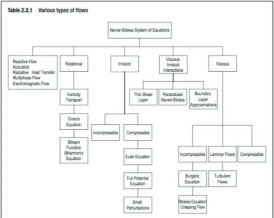
where g stands for gravity force, p stands for pressure, ⌫ for kinematic viscosity and ∆ is the laplacian operator. For all incompressible fluid flow simulations considered in this thesis, g is neglected and density is considered subsumed with the pressure term. An additional equation for conservation of energy is used for certain applications such as combustion and heat transfer flows - such flows are not considered in this thesis. The various types of fluid flows that can be expressed through modifications of the NS equations set is shown in figure 1.2.
Figure 1.2: Flow types that can be depicted by the Navier-Stokes equation set. Borrowed from Chung (2010).
1.1.3 Discretisation techniques
The non-linearity of the term u · ∇u makes the analytical solution of the NS equation unachievable for all but the simplest of fluid flow problems. Thus, practical solutions of the NS equations can only be obtained, at present, by computational simulations using a discretised form of the equations. This section expands on existing numerical discretisation techniques.
Finite difference method
In finite difference methods (FDM), the partial differential equations (PDE) to be solved are approximated using difference equations within which the derivatives are expressed through finite differences. The expression for the derivatives of a function f(x) around a point x0 can be derived from Taylor’s polynomial:
f (x0+ h) = f (x0) + f (x0) 1! h + f(2)(x0) 2! h 2+ ... + R n(x), (1.1.4)
where h is the step size, and Rn(x) stands for the higher-order expansions beyond the order
n expressed by the equation. The derivative can thus be expressed as, f (x0) =
f (x0+ h) − f (x0)
h , (1.1.5)
Many numerical methods can be envisaged to approximate the derivatives. For a ve-locity field u in 1D space x with a step size of dx , the simplest approximations are, Forward difference: @ui @x = ui+1− ui dx + O(dx), (1.1.6) Backward difference: @ui @x = ui− ui−1 dx + O(dx), (1.1.7) Central difference: @ui @x = ui+1− ui−1 2dx + O(dx 2), (1.1.8)
Second order derivative: @2u i @x2 = ui+1− 2ui+ ui−1 dx2 + O(dx 2), (1.1.9)
where O stands for neglected higher order terms, and i is an index corresponding to the point on which the derivates are being expressed.
Similarly any order of derivatives can be derived from Taylor’s approximation using any specific number of points. These formulae can also be expanded easily to 2D and 3D. For example, the laplacian in 2D for an equi-spaced mesh can be expressed as,
∆uij =
ui+1,j + ui−1,j + ui,j+1+ ui,j−1− 4ui,j
dx2 + O(dx
4, dy4), (1.1.10)
where i and j are indices in 2D for the x and y directions respectively.
The accuracy of a finite difference scheme is assessed in three ways. The scheme is consistent if the approximation tends to the partial differential equation as the grid size is reduced. The scheme is considered stable if its error remains bounded. Finally, the results of a convergent scheme approach the results of the original equation as the grid size approaches zero. The advantage of FDM lies in its intuitive nature and ease of formu-lation. However, implementation becomes difficult with complex geometries and moving boundaries.
Finite volume method
The finite volume method (FVM) provides an alternative to FDM for spatial discreti-sation where the integral form of the equation set is reduced to a set of ordinary differential equations (ODEs). FVM is used commonly in the field of CFD due to the conservative nature of the resultant equations as well as their applicability to unstructured, irregular meshes without any coordinate transformation.
Given a conservation equation of Q over a volume V , @Q
@t + r · F = P r, (1.1.11)
with F denoting the flux of Q per unit volume per unit time and P r the production rate of Q, its integral form can then be written as,
d dt Z V (t) QdV + I S(t) n · F dS = Z V (t) (P r)dV. (1.1.12)
To solve this integral form, the volume V is broken into multiple control volumes which collate to form the total volume V . For each control volume, certain approximations are applied to calculate the value of Q and thus the flux F at the boundary of each volume along with the production P r within the volume. A time marching scheme is then applied to advance the solution of Q in time.
Finite element method
Finite element method (FEM) was first introduced in the field of structural mechanics and was later adopted for solving fluid flow problems especially when complex geometry was involved. The ability of the method to decompose the domain into smaller elements or finite elements of flexible geometry highlights the main advantage of the FEM. In addition, in FEM, the weak form of the governing equation is approximated unlike FDM/FVM where we work with the strong form of the governing equations. This allows the ability to provide higher order of approximations as well as flexibility in the implementation of boundary conditions. The weak form is obtained by the inner product of the residual of the governing equations and chosen test functions/basis functions. Such an equation represents the orthogonal projection of the residual error onto the test functional subspace integrated over the domain. Equating this to zero minimises the error functional thus providing the best approximation of the solution to the governing equation. While FEM are effective for structural problems, in the field of CFD involving a large number of grid points, the use of simpler schemes with a lower order approximation such as FDM/FVM is preferred. FEM within CFD is generally applied in the case of complex geometries mainly with industrial applications. For more information about different discretisation techniques with examples, please refer to Chung (2010); Pulliam and Zingg (2014).
1.1.4 Boundary conditions
Boundary conditions play an important role in CFD. They define the behaviour of the fluid at the boundaries outside of which no information of the fluid flow is known. Thus these conditions need to be defined accurately in space and for transient cases, an additional condition defining the flow at the initial time step is required. An error in the boundary condition can lead to errors in simulation as well as cause issues in convergence and stability of the simulation. In general, the boundary condition can take one of three forms: for a Dirichlet condition, a value for the function is defined at the boundary, while for a Neumann condition, the normal derivative of the function at the boundary is defined and a combination of the two is defined as the Robin boundary condition. Common boundary conditions for CFD (for velocity fields) are:
• Inlet condition defines the value of the fluid flow velocity at the inlet boundary. Wake flows, channel flows, and pipe flows are a few example which use the inlet boundary condition.
• Outlet condition defines the value of the fluid flow velocity at the outlet boundary when this velocity field is known. Channel flows, and pipe flows are a few example which use the outlet boundary condition.
• No slip condition is used to define the velocity at solid boundaries such as the wall of a channel flow. The normal component of the velocity is set to zero while the tangential component is set to the wall speed. The boundary on the cylinder, the walls of a channel or pipe are examples where the no slip condition is implemented. • Constant pressure condition defines the value of pressure usually at inlet or outlet
boundaries especially when the velocity field is unknown. Buoyancy driven flows, free surface flows, and flows around buildings are examples which can employ the constant pressure condition.
• Periodic condition are applied in flows where a repeated flow pattern is observed along a given direction. This condition is applied for the theoretical Taylor-Green vortex simulations, as well as in channel flow for inlet/outlet boundaries and for wake flows in the spanwise direction of the cylinder.
1.1.5 Turbulence modelling
To accurately simulate a fluid flow, all the length and time scales of the fluid need to be resolved explicitly by the discretisation mechanism employed. However, for the case of turbulent flows, the range of length scales increases exponentially with the Reynolds number and is, in general, computationally prohibitive to resolve all of these scales in a simulation. Thus, an alternative approach is required to model the smaller scales of turbulent motion which are not captured by the discretisation method. Such an approach is referred to as turbulence modelling. A simulation resolving all the scales of motion is referred to as a direct numerical simulation (DNS) and is the most accurate form of simulation possible - DNS results are used as a reference to assess model performance. Depending on the range of scales resolved by the simulations, and equivalently, the range of scales modelled by a model, the classification of the turbulence model can be done. Large eddy simulations resolve most of the turbulent scales while modelling the smallest scales removed from the flow by a filtering mechanism. In the Reynolds-Averaged Navier-Stokes equations, which is the oldest approach to turbulence modelling, the time-averaged velocity field is obtained by simulating the time-averaged governing equations where the contribution of the fluctuation components are expressed through additional terms known as Reynolds stresses which need to be modelled. A more detailed study of turbulence modelling is presented in chapter 2 elaborating on LES and RANS models as well as other methods available in literature.
1.2
Experimental fluid dynamics
1.2.1 A brief history of EFD
A succinct and well-written history of the major contributors and their contributions to fluid dynamics, as we know it, is provided by Anderson (2010). Here, I summarise in brief the contribution related to the field of experimental developments for fluid flow measurement. The first diagram of flow streamlines around an object dates back 500 years to Leonardo Da Vinci. He also stated vaguely the continuity equation for low-speed flows as well as stating the ’wind-tunnel principle’ - the relative flow over a stationary body mounted in a wind-tunnel is the same as the relative flow over the same body moving through a stationary fluid. Following this, experiments on fluids were conducted on fluid statics during the 17-18th century. An important advancement to the field of EFD is the invention of the Pitot tube by Henri Pitot in the year 1732. The Pitot tube is capable of measuring the flow velocity at a point within the fluid and is still a commonplace equipment in any fluids laboratory. The study of turbulent flows is attributed to the famous experiments of Osborne Reynolds who studied the flow of fluids in a pipe and the effect of varying parameters on this flow by releasing a dye in the stream. His study on the flow variation with parameters led to the famous non-dimensional Reynolds number used to segregate a flow into laminar or turbulent. Another prominent example in the field of flow measurement is the experiments of Prandtl in 1904, where he studied the boundary layer as well as flow separation characteristics behind solid bodies in a flow using a water channel. Since the experimental attempts of Reynolds and Prandtl, technical advances in
the associated fields of optics, computers, electronics, image and signal processing, among others, has revolutionised measurement techniques for EFD. A few established techniques are discussed in successive sections.
1.2.2 Hot wire anemometry (HWA)
HWA was first introduced in the early 20th century before being commercialised mid-century and is one of the fundamental tools used for measuring point-wise velocity fields especially in turbulent flows. HWA calculates velocity based on the amount of cooling induced by the flow on a heated sensor maintained at a constant temperature by a feedback-control loop. The voltage drop across the sensor required to maintain equilibrium is used to measure the instantaneous velocity of the flow. As the velocity over the sensor changes, the corresponding convective heat transfer coefficient varies leading to a different voltage drop necessary to maintain equilibrium. Figure 1.3 depicts the electrical circuit diagram for HWA. The heat transfer from the sensor is not just a function of the flow velocity but also its geometry, orientation, the flow temperature, and concentration. Thus, it is possible to measure with HWA other fluid parameters such as concentration (Harion et al., 1996), temperature (Ndoye et al., 2010), as well as the individual components of the velocity field. Newer designs of probes are capable of measuring simultaneously all three velocity components. In addition, HWA’s capability for high data-gathering rate of the order of several hundred kHz as well as the very small size of the sensor which minimises disturbance of the measured flow are distinct advantages of HWA over other intrusive flow measurement techniques. However, a stringent need for calibration, as well as the possibility of contamination/breakage due to fragility of the sensor limit application of HWA to all flows.
Figure 1.3: Circuit diagram for hot-wire anemometer.
1.2.3 Laser doppler anemometry (LDA)
The Doppler effect refers to the change in frequency or wavelength of a given wave signal when the relative velocity between the source and the observer varies. This shift is exploited in LDA to measure the velocity of a flow by illuminating it with a laser beam
which are reflected/scattered by particles seeded into the flow. The frequency difference between the original incident beam and the scattered beam, the Doppler shift, is linearly proportional to the particle velocity. The non-intrusive nature of LDA along with the high spatial and temporal resolution of the method and its ability to perform multi-component measurements are intrinsic advantages of LDA. However, its application is limited to ar-eas with optical access, and single-point mar-easurements. Seeding particles and seeding concentration are important factors which affect the performance of LDA. Depending on the optical arrangement of the Laser and the receiver, LDA can be classified as forward-scattering, side-forward-scattering, or back-scattering LDA with the last being the most preferred option in modern set-ups. One such commercial set-up for an LDA experiment is shown in figure 1.4 - the fringe mode of LDA measurements is employed here by splitting the laser into two beams using a Bragg cell which intersect in the measurement zone. The frequency shift between the two intersection laser beams, induced due to their different incident angles, is used to calculate the Doppler frequency which is directly proportional to velocity.
Figure 1.4: Laser Doppler Anemometer measurement set-up. Obtained froma
1.2.4 Particle image velocimetry (PIV)
Both HWA and LDA are point-wise flow measurement techniques capable of measuring velocity with good temporal resolution at a given point in a flow. However, there is a strong need for full field (both 2D and 3D) velocity measurements - this was the motivation behind the development of PIV techniques. The development of PIV was done by Adrian (1984) under the name pulsed light velocimetry. This was followed by variants of the technique
proposed by Lourenco and Krothapalli (1986); Willert and Gharib (1991); Westerweel (1994) under different names although all these methods now fall in the PIV category. Since it’s development, PIV has become the dominant method for fluid flow measurement and remains till date the most popular method for turbulent flow measurement. The dominance of PIV can be attributed to the robustness of the method which arises from the simplicity of concept behind PIV. Adrian and Westerweel, two pioneers in the field of PIV, explain that the ability of PIV to directly measure displacement and time increment, which combined define the velocity field, provides robustness to the method. Adding to this, the ability of PIV to provide fields of velocity measurements and using particles as markers (omnipresence of particles and their ability to scatter more light compared to dye or molecules) are important characteristics. The art of particle imaging and processing can occupy entire textbooks, but for the purpose of this thesis, only a precise introduction to PIV principles and its extension to 3D flows (Tomographic PIV or recently 4D-PTV) is relevant and forms the core of this section.
Figure 1.5 is a schematic of basic planar PIV systems consisting of a double-pulsed laser, optics system, particle seeding, camera system, image processing software, and associated hardware for storage. A double-pulsed laser, generally a solid-state Nd:YAG laser, is used to produce two laser pulses to illuminate the flow which is seeded using the particle seeder with flow tracer particles, such as oil droplets in air or titanium dioxide in fluids. Newer methods have been developed which use helium filled soap bubbles as tracer particles (Schneiders et al., 2016) whose large size allow lasers of lower intensity to be used in the experiments. The reflected light is then captured using a camera-lens setup, digitised and then processed by an image processing software to improve quality, de-noising, etc. The next and an essential feature of PIV technique is the measurement of particle displacement between two consecutive images. This step, referred to as image or displacement interrogation, calculates from the image data particle displacements and thus flow velocity, using interrogation windows. A general method is the correlation technique where the image is split into interrogation windows of custom pixel size over which particle displacement correlation is performed using appropriate algorithms to identify the flow velocity for the window. This represents a large-scale view point of the flow and for highly turbulent flows, it fails to capture the small scale turbulent structures. A thorough description of PIV techniques can be found in any of the books dedicated to the subject.
Arroyo and Greated (1991) installed two cameras in their PIV set-up making it capable of measuring not just the two in-plane velocity components but also the out-of-plane com-ponent using the concept of stereoscopic imaging. Such a method, named stereoscopic PIV (SPIV), has certain advantages as it eliminates perspective error of monoscopic imaging, provides the full velocity vector field, and requires only an additional camera and corre-sponding calibration. Of particular interest to experimentalists is the ability to measure the full velocity vector over a volumetric domain. Different PIV techniques are capable of achieving this: Swept-Beam PIV (Gray et al., 1991) sweeps the planar light sheet over the volumetric domain, however, the measured field is not instantaneous. Photogrammetric PTV (Kent et al., 1993) uses multiple cameras to determine the 3D position of particles over two or more consecutive snapshots but is limited to large-sized tracer particles and associated flows. Holographic PIV (Fabry, 1998; Soria and Atkinson, 2008) uses princi-ples of holographic recording and reconstruction to obtain volumetric measurements using SPIV like correlation algorithms but the method is limited to very-small volumes due to high-resolution requirements, Tomographic PIV (Elsinga et al., 2006) uses photogrammet-ric PTV like set of cameras (minimum 4 cameras) to record double-frame images and mathematically reconstruct the volume by projecting the image pixel gray-levels back into
Figure 1.5: 2D Planar PIV system schematic representation (Westerweel et al., 2013). the fluid and combing projections as and when they intersect. This is followed by a three-dimensional correlation analysis to interrogate the volume. Tomo-PIV is limited due to high computational costs and limited volumetric size but has been increasingly applied to measure the three components of flow velocity within a 3D volume (3D-3C) producing re-warding results (Hain et al., 2008; Kim and Chung, 2004; Weinkauff et al., 2013). The use of Helium-Filled Soap Bubbles (HFSB) as tracer particles has enabled a considerable in-crease in the measured volume size to a cubic-meter. The large size of these particles leads to increased light scattering and sparse seeding enabling large-scale measurements. Other innovative 3D measurement and reconstruction techniques include Tomo-PTV (Schneiders and Scarano, 2016), Shake The Box (Schanz et al., 2016), Holographic PTV, Vortex-in-cell (VIC) (Schneiders et al., 2014), etc.
1.3
Limitations
Both CFD and EFD have been extensively used to study fluid flows over the past century. However, there are associated drawbacks with each method which affect the accu-racy of flow representation. CFD simulates a numerical approximation of the mathematical equations describing the flow. When the exact governing equations are known, an accurate approximation is in principle possible. However, for many cases the exact equations are unknown necessitating the introduction of a model introducing model errors. Even when exact equations are available, models are still used to reduce computational cost (turbu-lence modelling), which introduces model errors. Discretisation errors are introduced by the discretisation methods employed (FDM/FEM/FVM) in the form of truncation and
round-up errors. These can be minimised by using more complex schemes but at the cost of increased computational time. The use of iterative methods could also lead to numerical errors if sufficient iterations are not performed for convergence. Errors are also introduced due to inaccurate descriptions of the boundary conditions and initial conditions which are complex for realistic turbulent flows. Even for simple turbulent flows such as channel flow or wake flow around a cylinder, an accurate, realistic turbulent inlet/initial condition is difficult to envisage. Errors increase due to approximations or simplifications used to describe these conditions. Clearly, all these factors need to be taken into account when simulating any fluid flow. A compromise is generally required between computational cost and accuracy.
EFD methods are capable of capturing realistic flows which are, as of now, out of reach of CFD simulations. However, there are major limitations when it comes to ex-perimental measurement techniques. Point-wise measurement techniques are capable of measuring accurate time-resolved fields but are severely limited in spatial extent. Even for 2D measurement techniques such as PIV, the measurement size is limited due to optical restrictions. The lack of sophisticated techniques to measure fluid properties over a large volumetric domain remains a major limitation of EFD techniques. Existing 3D measure-ment techniques are limited either to small volumetric domains or to non-instantaneous profiles (as obtained from swept-beam PIV) due to prohibitive costs for working the laser. The spatial resolution of measurements for PIV, SPIV and Tomo-PIV are all limited to large-scales especially for turbulent flows. Apart from the spatial limitations, the inabil-ity of EFD methods to simultaneously measure multiple properties of the fluid (velocinabil-ity, pressure, temperature, density, etc.) is a major drawback.
1.4
Coupling EFD and CFD
An analysis of the limitation and abilities of CFD and EFD indicates a certain amount of complementarity between them. CFD is limited by the accuracy of its inlet and initial conditions, while EFD is capable of measuring an accurate initial and inlet conditions. EFD is limited in spatial extent while a large domain can be easily simulated using CFD. EFD is capable of measuring accurate but sparse and selective flow field properties while CFD is capable of measuring an approximated but complete flow-field properties over a large domain. The exploitation of this complementarity is a classic tradition in the field of fluid mechanics where experimental measurements are used to validate CFD results. Recently, this complementary has attracted more attention for possible coupling of EFD and CFD by using a dynamical model guided by partial or sparse experimental observations. Such a coupling, referred to as Data Assimilation, within the context of fluid mechanics is the primary focus of this thesis. A brief introduction to DA is provided here while a technical discussion can be found in chapter 5.
DA, as a field, has been driven by the works of researchers from the atmospheric and oceanographic sciences as well as contribution from geosciences. The need for DA was realised well before computers and numerical solvers were invented, in the year 1913 by Lewis Fry Richardson. He was working in the field of weather prediction and aimed at representing the physical principles governing the atmosphere as a set of mathematical equations which could be solved numerically. Richardson solved these equations manually with the available sparse observation set to disastrous results (Lynch, 2008). He realised that his erroneous results were due to an incorrect initial condition and concluded that a cure would be to initialise the numerical method with more realistic and complete set of observations, i.e. data assimilation. The sensitivity of atmospheric systems to the
initial condition is an important backdrop to the origination of DA techniques within the field of atmospheric sciences. With the invention of computers, a deeper understanding of physical principles governing the system, and more stable algorithms, the field of DA has come forward with leaps and bounds.
The current version of DA procedures can be broadly categorised into two main gories. Methods which are derived from stochastic filtering principles fall under the cate-gory of sequential data assimilation (SDA) approaches. The particle filter method (Gordon et al., 1993), the Ensemble Kalman Filter (EnKF) (Evensen, 1994), or a combination of both methods (Papadakis et al., 2010) are prominent examples of this method. These methods are generally based on the principle of Bayesian minimum variance estimation. They are termed as ‘sequential’ due to the constant forward propagation of the system state. As and when observations are encountered, they are assimilated into the system to correct the predicted state.
The second category of DA procedures are referred to as variational data assimilation (VDA) approaches and these originate from concepts of optimal control theory and varia-tion calculus thus deriving the name (Lions, 1971). These methods aim at estimating the optimal trajectory, starting from a background condition, which minimises a cost function leading to lowest error between system and observations. The works of Bergthórsson and Döös (1955); Cressman (1959) on Optimal Interpolation methods were stepping stones to the VDA methods. With VDA, the approaches can be declassified into 3D variational and 4D variational methods depending on the spatial dimensions of the simulation and the inclusion or not of a temporal window for the system’s dynamical evolution. A first application of such methods was done by Sasaki (1958) who further extended them to 4D analysis in Sasaki (1970). Since then, variants of the VDA approach has been used for DA with Le Dimet and Talagrand (1986); Gronskis et al. (2013) being some prominent examples.
While SDA and VDA methods are inherently based on different principles, an equiva-lence between the two can be drawn for specific cases as shown by Li and Navon (2001); Yang (2014). In adherence to the essence of DA towards combining complementary meth-ods, the work of Yang et al. (2015) combines the ensemble Kalman filter approach with the 4D-Var method to provide a hybrid methodology. This is built on the publication of Hamill and Snyder (2000) who combined an ensemble based background covariance with 3D variational methods and Lorenc (2003) who expanded it to 4D. A different set of hybrid techniques which are based on SDA approaches incorporating variational formalisms were developed and analysed by Hunt et al. (2004, 2007); Fertig et al. (2007).
The various methodologies developed over the last decade for studying fluid flows in the fields of EFD, CFD and DA are graphically shown in figure 1.6. A stagnation can be seen in the development of methodologies which are restricted to a single field of focus namely EFD or CFD. 3D-PIV for EFD and stochastic NS/LES for CFD are the only major developments in the respective fields over the past decade. The data assimilation domain, however, has clearly attracted major research interest with increasing number of publications. Even within experimental methodologies, a shift towards combinatory techniques can be seen with techniques such as VIC (Schneiders et al., 2014), VIC+ (Schneiders et al., 2016), FlowFit Gesemann et al. (2016), etc.
In this present work, the VDA approach developed by Gronskis et al. (2013) for 2D DNS of cylinder wake flow and extended to 3D DNS of wake flows by Robinson (2015) (termed henceforth as 4D-Var) is expanded to account for an LES turbulence model. Such an approach should be capable of performing VDA on flows of higher Reynolds numbers