HAL Id: tel-00276848
https://tel.archives-ouvertes.fr/tel-00276848
Submitted on 2 May 2008HAL is a multi-disciplinary open access
archive for the deposit and dissemination of sci-entific research documents, whether they are pub-lished or not. The documents may come from teaching and research institutions in France or abroad, or from public or private research centers.
L’archive ouverte pluridisciplinaire HAL, est destinée au dépôt et à la diffusion de documents scientifiques de niveau recherche, publiés ou non, émanant des établissements d’enseignement et de recherche français ou étrangers, des laboratoires publics ou privés.
Contribution à l’approximation de problème
d’identification et décomposition de domaine en
élasticité.
Abdellatif Ellabib
To cite this version:
Abdellatif Ellabib. Contribution à l’approximation de problème d’identification et décomposition de domaine en élasticité.. Mathématiques [math]. Faculté des Sciences et Techniques de Marrakech, 2008. �tel-00276848�
HABILITATION UNIVERSITAIRE
Présentée à la Faculté des Sciences et Techniques – Marrakech
UFR : Mathématiques et Informatique
Spécialité : Mathématiques Appliquées et Informatique
CONTRIBUTION À L’APPROXIMATION DE PROBLÈME
D’IDENTIFICATION ET DÉCOMPOSITION
DE DOMAINE EN ÉLASTICITÉ
Par :
Abdellatif ELLABIB
(Doctorat : Mathématiques Appliquées
)
Soutenue le 15 Mars 2008 devant la commission d’examen :
Président :
M. Ali Souissi, Professeur Faculté des Sciences-Rabat
Examinateurs :
M. Noureddine Alaa, Professeur Faculté des Sciences et Techniques – Marrakech M. Abdelilah Hakim, Professeur Faculté des Sciences et Techniques – Marrakech
M. Abdeljalil Nachaoui, Maître de Conférences HDR Faculté des Sciences et Techniques – Nantes, France.
M. Jean Rodolophe Roche, Professeur Institut Élie Cartan – Nancy, France.
UNIVERSITE CADI AYYAD
FACULTE DES SCIENCES ET
TECHNIQUES-MARRAKECH
N° d’ordre 03/2008
À MES PARENTS
À TOUTE MA FAMILLE
Remerciements
Ce travail de recherche a été réalisé au Laboratoire de Mathématiques Jean
Leray de l’université de Nantes et au Laboratoire de Mathématiques Appliquées
et Informatique de l’université Cadi Ayyad. Je remercie tout d’abord tous les
membres du Laboratoire de Mathématiques Jean Leray de l’université de Nantes
pour les différentes invitations.
Pour m’avoir fait l’honneur de présider ce jury, je remercie Monsieur Ali
Souissi, Professeur à la Faculté des Sciences de Rabat.
J’exprime ma profonde reconnaissance et gratitude à Monsieur Abdeljalil
Nachaoui, Maître de Conférences HDR à la Faculté des Sciences et Techniques
de Nantes, d’abord en tant que mon directeur de thèse de doctorat de l’université
de Nantes puis en tant que collaborateur scientifique, de m’avoir fait profiter de
son expérience et ses grandes compétences scientifiques. Sa disponibilité
permanente, lors de mes séjours à Nantes, et ses qualités humaines ont été un
grand atout pour mener à bien ces travaux, je le remercie également d’avoir
accepté de faire partie du jury, malgré ses multiples obligations.
J’adresse mes sincères remerciements à Monsieur Noureddine Alaa, Professeur
à la Faculté des Sciences et Techniques de Marrakech et Monsieur Jean
Rodolphe Roche, Professeur à l’Institut Élie Cartan de Nancy de l’honneur
qu’ils m’ont fait en acceptant de rapporter sur cette habilitation et de se joindre
au jury.
Je remercie vivement Monsieur François Jauberteau, Professeur à la Faculté des
Sciences et Techniques de Nantes, d’avoir accepté de rapporter sur ce manuscrit.
Je remercie Monsieur Abdelilah Hakim, Professeur à la Faculté des Sciences et
Techniques de Marrakech, d’avoir accepté de faire partie du jury.
Mes amis et collègues de la Faculté des Sciences et Techniques de Marrakech
qu’ils trouvent ici l’expression de ma gratitude et de ma sympathie.
J’exprime ma sincère reconnaissance à tous ceux qui m’ont aidé à réaliser ce
travail.
FICHE PRESENTATIVE DE L’HABILITATION UNIVERSITAIRE
Nom et Prénom de l’auteur : ELLABIB Abdellatif
Intitulé des travaux de recherche : Contribution à l’approximation de problème
d’identification et décomposition de domaine en élasticité
Professeur responsable :
Monsieur Abdelilah Hakim Professeur à la Faculté des Sciences et Techniques de Marrakech.
Lieux de réalisation des travaux de recherche :
Laboratoire Mathématiques Appliquées et Informatique de l’université Cadi Ayyad
de Marrakech et Laboratoire Jean Leray de l’université de Nantes.
Période de réalisation des travaux de recherche :
Du Juin 2003 au Novembre 2007
Rapporteurs :
Monsieur Alaa Noureddine; Professeur de l’enseignement supérieur;
Université Cadi Ayyad, Faculté des Sciences et Techniques
B.P. 549 Guéliz – Marrakech, Maroc
Monsieur Jauberteau François; Professeur;
Université de Nantes, Faculté des Sciences et Techniques,
B. P. 92208, F44322 Nantes cedex 3, France.
Monsieur Roche Jean Rodolphe; Professeur;
Institut Élie Cartan,
B.P. 239, 54506 Vandouvre-lès-Nancy Cedex, France.
Cadres de coopération :
Coopération scientifique entre le Laboratoire de Mathématiques Appliquées et Informatique
de la Faculté des Sciences et Techniques de Marrakech et le Laboratoire de Mathématiques
Jean Leray de l’université de Nantes et les Actions intégrées N° MA/05/116 et MA/07/164.
Ce travail a donné lieu aux résultats suivants :
Deux publications dans des journaux internationaux avec comité de lecture et un article
soumis à un journal international et trois communications dans des congrès internationaux
avec comité de lecture et un encadrement en mémoire de DESA et deux polycopiés de cours
Table des mati`
eres
1 Introduction 1
2 Research Report / Pr´esentation des travaux de recherches 8
2.1 An iterative approach to the solution of an inverse problem in linear elasticity 9
2.1.1 Introduction . . . 9
2.1.2 Mathematical model . . . 10
2.1.3 Description of the alternating algorithm . . . 11
2.1.4 Integral equation formulation and boundary element . . . 14
2.1.5 Implementation . . . 16
2.1.6 Numerical results . . . 18
2.2 A domain decomposition method for boundary element approximations of the elasticity equations . . . 25
2.2.1 Introduction . . . 25
2.2.2 Domain decomposition techniques . . . 26
2.2.3 Integral equation formulation and boundary element for elasticity equations . . . 28
2.2.4 Algebraic systems of Dirichlet Neumann and Schwarz methods . . . 28
2.2.5 Numerical results and discussions . . . 32
2.3 A domain decomposition convergence for elasticity equations . . . 38
2.3.1 Introduction . . . 38
2.3.2 Optimal control formulation . . . 39
2.3.3 Existence of optimal solution . . . 40
2.3.4 Approximation of the problem . . . 41
2.3.5 Convergence result . . . 44
2.3.6 Optimization algorithm . . . 46
2.3.7 Numerical results . . . 48
3 Papers / Liste des publications 53 3.1 Articles parus/`a paraˆıtre dans des revues internationales . . . 54
3.2 Articles dans des congr´es internationaux avec actes et comit´e de lecture . . 54
4 Project and other research activities / Projet et autres activit´es de
recherches 56
5 Teaching Report / Activit´es d’enseignements 61
6 Papers joints / Articles joints 68
Chapitre 1
Introduction
Introduction (version fran¸caise)
Dans ce document de synth`ese, nous d´ecrivons principalement les activit´es de re-cherches entam´es depuis Juin 2003 et les activit´es d’enseignements. Nous pr´esentons tout d’abord des travaux de recherches qui ont ´et´e achev´es et dont les probl´ematiques n’´etaient pas abord´ees dans ma th`ese de Doctorat de l’universit´e de Nantes, ensuite une liste de publication, diff´erents projets et d’autres activit´es de recherches et enfin un curriculum vitae.
Les travaux de recherches pr´esent´es sont divis´es en deux axes. Le premier axe concerne le probl`eme d’identification de donn´ees en ´elasticit´e lin´eaire. Le deuxi`eme axe de recherche est consacr´e `a la m´ethode de d´ecomposition en sous-domaines.
Nous consid´erons un corps ´elastique qui occupe une r´egion ouverte Ω de fronti`ere Γ = Γ1∪ Γ2 et Γ1∩ Γ2 = ∅.
Notons f la densit´e volumique de forces dans Ω. Les champs de d´eplacements u = (ui) et
de contraintes σ = (σij) satisfont les ´equations suivantes [8].
´ Equation d’´equilibre : ∂σij ∂xj = f dans Ω (1.1) ´ Equation de comportement : σij = aijkhεkh(u) (1.2) εkh(u) = 1 2 µ ∂uh ∂xk +∂uk ∂xh ¶ . (1.3)
Les termes aijkh(x) sont appel´es les coefficients d’´elasticit´e.
Dans le cas des mat´eriaux ´elastiques isotropes, ces coefficients aijkhs’expriment en fonction
de λ et µ par
aijkh = λδijδkh+ µ(δikδjh+ δihδjk) (1.4)
o`u λ et µ sont les coefficients de Lam´e et δij est le symbole de Kronecker.
En injectant, l’´equation de comportement (1.2) dans l’´equation d’´equilibre (1.1) et en combinant l’´equation (1.3) et la relation (1.4), nous obtenons alors l’´equation d´ecrivant les champs de d´eplacement suivante.
G ∂ 2u i ∂xj∂xj + G 1 − 2ν ∂2u j ∂xi∂xj = f dans Ω (1.5)
o`u G et ν d´esignent respectivement le module de Shear et le coefficient de Poisson. Dans cet axe de recherche, nous nous int´eressons `a l’approximation num´erique d’un probl`eme inverse en ´elasticit´e lin´eaire. Nous cherchons `a identifier des conditions aux limites inaccessibles `a la mesure sur la partie Γ2 de la fronti`ere du domaine Ω connaissant
des mesures de d´eplacement et de forces sur la partie compl´ementaire Γ1 de la fronti`ere
du domaine Ω. Le mod`ele math´ematique d´ecrivant ce probl`eme d’identification est form´e par l’´equation (1.5) et les conditions aux limites suivantes
ui = ˜ui sur Γ1 (1.6)
et
ti = ˜ti sur Γ1 (1.7)
o`u ˜u et ˜t sont des fonctions donn´ees.
Ce probl`eme obtenu est mal pos´e au sens de Hadamard [19], la solution est instable, elle change rapidement pour une petite modification des donn´ees.
Nous transformons le probl`eme (1.5), (1.6), (1.7) en appliquant l’algorithme de re-construction des conditions aux limites introduit dans [34]. Cette m´ethode se base sur la r´esolution d’une suite de probl`emes d’´equations aux d´eriv´ees partielles bien pos´es. L’approximation num´erique des diff´erents probl`emes se fait par les ´el´ements de fronti`eres [4]. Ces ´el´ements g´en`erent des syst`emes lin´eaires de matrices denses, non-sym´etriques et mal conditionn´es, nous utilisons alors des m´ethodes [41, 42] de r´esolution adapt´ees `a un tel syst`eme lin´eaire. Des essais num´eriques pour des probl`emes bidimensionnels seront pr´esent´es.
Notre travail qui utilise les m´ethodes de d´ecomposition en sous-domaines a d´emarr´e en 2004.
Dans le deuxi`eme axe de recherche, nous nous int´eressons `a l’application de la m´ethode de d´ecomposition en sous-domaines `a un probl`eme direct d´ecrivant les ´equations d’´elasticit´e lin´eaire. Ce probl`eme est form´e des ´equations (1.5), (1.6) et une condition aux limites sur Γ2
ti = ˜ti sur Γ2 (1.8)
o`u ˜t est une fonction donn´ee sur Γ2.
Notre premier objectif de cet axe est d’approcher le probl`eme (1.5), (1.6) et (1.8) en appliquant les m´ethodes de d´ecomposition de domaine [37]. Nous utilisons une m´ethode de d´ecomposition sans recouvrement et la m´ethode de Schwarz coupl´ees avec une approxi-mation par les ´equations int´egrales et les ´el´ements de fronti`eres. Cette approxiapproxi-mation ne necessite que la discr´etisation de la fronti`ere de chaque sous-domaines et elle permet de r´eduire le nombre d’inconnues et le temps de calcul. Nous pr´esentons en d´etail les algo-rithmes de Dirichlet-Neumann et Schwarz. Nous d´ecrivons les syst`emes alg´ebriques issus des m´ethodes de d´ecomposition avec recouvrement et sans recouvrement. Nous pr´esentons ensuite deux algorithmes et des r´esultats num´eriques qui illustrent la convergence de ces
deux algorithmes vers la solution du probl`eme d’´elasticit´e lin´eaire dans diff´erents do-maines.
Enfin, Nous ´etudions une m´ethode de d´ecomposition du domaine sans recouvrement pour les ´equations d’´elasticit´e. Cette m´ethode est bas´ee sur la formulation du probl`eme en un probl`eme de contrˆole optimal. Nous d´emontrons l’existence de la solution et la conver-gence de la solution de probl`eme approch´e vers la solution du probl`eme continu. Nous exposons un algorithme d’optimsation en utilisant le Lagrangien. Enfin, nous pr´esentons les r´esultats num´eriques qui montrent l’efficacit´e de notre algorithme et confirment le r´esultat de convergence.
Introduction (English version)
In this document, we describe the research activities started since June 2003 and lessons activities. We present research work which had been completed and that the issues were not addressed in my thesis at the University of Nantes.
This work is divided into two lines of research. The first axis concerning the problem of identification data linear elasticity. The second line of research is devoted to domain decomposition method.
We consider an isotropic linear elastic material which occupies an open bounded do-main Ω with boundary Γ = Γ1∪ Γ2 and Γ1∩ Γ2 = ∅.
Let f the body forces, the displacement u = (ui) and constraints σ = (σij) satisfy the
following equations [8]. Equilibrium equation :
∂σij
∂xj
= f in Ω (1.9)
The stress σij are related to the strains through the
Constitutive law : σij = 2G µ εij + ν 1 − 2νδijεkk ¶ (1.10) where G and ν are the shear modulus and Poisson ratio, respectively and δij is the
Kronecker delta tensor.
The strains εij are related to the displacement gradients by the kinematic relations
εij(u) = 1 2 µ ∂ui ∂xj +∂uj ∂xi ¶ . (1.11)
Now, we substitute the constitutive law (1.10) into the equilibrium equation (1.9), and use the kinematic relations (1.11), we obtain the following Navier equations.
G ∂2ui ∂xj∂xj + G 1 − 2ν ∂2u j ∂xi∂xj = f in Ω (1.12)
In this work, we are interested by a reconstruction inverse problem where the geometry of the problem and the material constants are determined, but the boundary conditions are not completely known. This problem arises in cases where a portion of the boundary is
exposed to environmental conditions which can not be assessed due to physical difficulties or geometrical inaccessibility. The aim in the reconstruction inverse problem is to find the unknown boundary conditions based on the supplementary data provided on the boundary and/or the domain.
Consider the problem where no conditions are prescribed on Γ2 and assume that it is
possible to measure the traction vector on Γ1. The mathematical formulation of an inverse
problem consisting of equation (1.12) and boundary conditions
ui = ˜ui on Γ1 (1.13)
ti = ˜ti on Γ1 (1.14)
where ˜u and ˜t are prescribed quantities.
This problem obtained is ill-posed and we cannot use a direct approach. The solution is unstable with a respect to small perturbations in the data on Γ1.
We translate the problem (1.12), (1.13) and (1.14) by applying the reconstruction algorithm of boundary conditions introduced into [34]. This method is based on solving a sequence of well-posed boundary value problems. The numerical approximation of the various problems is used by the boundary element method [4]. These systems generate dense linear matrix, unsymmetrical and ill-conditioned, then we use methods [41, 42] resolution adapted to such a linear system. Numerical results in two-dimensional case will be presented.
In 2004, we are interested to use the domain decomposition method to direct problem of linear elasticity. This problem is given by (1.12), (1.13) and boundary condition for traction on Γ2
ti = ˜ti on Γ2 (1.15)
where ˜t is a given function.
The main goal of this second axis is to solve elasticity problems (1.12), (1.13) and (1.15) using a domain decomposition method [37] coupled with the boundary element method [4] on complicated 2-D geometries Ω where Ω is not necessarly circular or rectangular. The decomposition method we have selected is a non-overlapping technique and Schwarz me-thod. We decompose the domain Ω into a number of subdomains Ωi with Ωi is rectangular
or circular domain and the solution in the entire domain Ω is computed via sequences of solutions computed in the subdomains Ωi. We describe in details Dirichlet-Neumann and
Schwarz algorithms. We have chosen to associate it with the boundary element method. Indeed, it only requires the discretization of the boundaries of the subdomains. This tech-nique of coupling reduces the number of unknowns and the time of computing. Numerical examples in two dimensional case for some complicated 2-D domain configurations are also illustrated.
Also, in this axis we present also a non-overlapping domain decomposition method for elasticity equations based on an optimal control formulation. The existence of a solution
is proved and the convergence of a subsequence of the approximate solutions to a solution of the continuous problem is shown. The implementation based on lagrangian method is discussed. Finally, numerical results showing the efficiency of our approach and confirming the convergence result are given.
Chapitre 2
Research Report / Pr´
esentation des
2.1
An iterative approach to the solution of an
in-verse problem in linear elasticity
2.1.1
Introduction
A vast body of engineering experience shows that the theory of linear elasticity allows an accurate modeling of many natural or manufactured solid materials (civil engineering structures, transportation vehicles, machines, the Earth’s mantle, rocks mechanics [27]) and provides an essential tool for analysis and design.
When the governing system of partial differential equations, i.e. the equilibrium, consti-tutive and kinematics equations, have to be solved with the appropriate initial and boun-dary conditions for the displacement and/or traction vectors, i.e. Dirichlet, Neumann or mixed boundary conditions the associated problems are called direct problems and their existence and uniqueness have been well established. When one or more of the conditions for solving the direct problem are partially or entirely unknown then an inverse pro-blem may be formulated to determine the unknowns from specified or measured system responses.
The main type of inverse problems that arise in the context of linear elasticity, and more generally of the mechanics of deformable solids, are similar to those encountered in other areas of physics involving continuous media and distributed physical quantities, e.g., acoustics, electrostatics and electromagnetism. They are usually motivated by the desire or need to overcome a lack of information concerning the properties of the system (a deformable solid body or structure). It should be noted that most of the inverse problems are ill-posed and hence they are more difficult to solve than the direct problems. It is well known that they are generally instable, i.e. the existence, uniqueness and stability of their solutions are not always guaranteed, see e.g. Hadamard [19]. Identification of inaccessible boundary values (Cauchy problem in elasticity) is a classical example of inverse problem. This inverse problem, in which both displacement and traction boundary conditions are prescribed only on a part of the boundary of the solution domain whilst no information is available on the remaining part of the boundary, can be encountered in many situations [20, 43].
Recently, an approximate solution to the Cauchy problem for Poison equation has been determined by one of the authors, [22, 34], using an alternating iterative method which reduced the problem to solving a sequence of well-posed boundary value problems. Our goal in this paper is to extend this algorithm in conjunction with the boundary element method (BEM) to the Cauchy problem in elasticity.
2.1.2
Mathematical model
Direct problem statement
The mathematical formulation of the 2D elasticity problem in the case of an isotropic linear elastic material which occupies an open bounded domain Ω ⊂ R2 with boundary Γ such that Γ = Γ1∪ Γ2, Γ1, Γ2 6= ∅ and Γ1∩ Γ2 = ∅ is described as follows.
Let w = (u, v)T be the displacement vector and b the volume force vector. Here (., .)T
denotes the transpose of a vector or a matrix. Let us define the matrices
D = ∂ ∂x 0 ∂ ∂y 0 ∂ ∂y ∂ ∂x E = ∂ ∂x 0 0 ∂ ∂y ∂ 2∂y ∂ 2∂x C = 1 − ν ν 0 ν 1 − ν 0 0 0 1 − 2ν (2.1)
Then the strain vector ε = (ε11, ε22, ε12)T is given by
ε = Ew (2.2)
The strain tensor ε is related to the stress vector σ = (σ11, σ22, σ12)T by the constitutive
law
σ = 2G
1 − 2νCε (2.3)
where G and ν are respectively the Shear modulus and Poisson ratio. The equilibrium equations are given by
Dσ = b (2.4)
If we now substitute the constitutive law (2.3) into the equilibrium equation (2.4), and use the kinematic relations (2.2) of the elasticity tensor for an isotropic linear elastic material, we obtain the following Lam´e system or the Navier equations
G∆u + G 1 − 2ν µ ∂2u ∂x2 + ∂2v ∂x∂y ¶ = b1 in Ω G∆v + G 1 − 2ν µ ∂2u ∂x∂y + ∂2v ∂y2 ¶ = b2 in Ω (2.5)
The solution of Eqs. (2.5) must satisfy prescribed boundary conditions on the boundary Γ of the body, which are based either on the displacements u and v, or the boundary traction t and s. The boundary conditions can be written into the following types
u(X) = ˜u(X), v(X) = ˜v(X) for X ∈ Γ1 (2.6)
and
t(X) = ˜t(X), s(X) = ˜s(X) for X ∈ Γ2 (2.7)
where (t(X), s(X)) is the traction vector at a point X ∈ Γ2 with ˜u, ˜v, ˜t and ˜s prescribed
Reconstruction inverse problem
The knowledge of the geometry (the domain Ω) of the problem, the material constants
G and ν and the prescribed quantities ˜u, ˜v, ˜tand ˜s enable us to determine the displacement
vector w(x) and the strain and the stress tensors in the domain Ω. In this case the problem is called direct problem. Different inverse problems can be considered for this direct problem. In all cases, part of the data which is known for the well posed direct problem is not known. In order to find this unknown data, supplementary information have to be provided.
In this work, we are interested by a reconstruction inverse problem where the geometry of the problem and the material constants are determined, but the boundary conditions are not completely known. This problem arises in cases where a portion of the boundary is exposed to environmental conditions which can not be assessed due to physical difficulties or geometrical inaccessibility. The aim in the reconstruction inverse problem is to find the unknown boundary conditions based on the supplementary data provided on the boundary and/or the domain.
Consider the problem where no conditions are prescribed on Γ2 and assume that it
is possible to measure the traction vector on Γ1. This gives arise to the supplementary
boundary conditions
t(X) = ˜t(X) and s(X) = ˜s(X) for X ∈ Γ1 (2.8)
where ˜t and ˜s are given functions.
In the next section, we describe an iterative method to solve numerically the recons-truction problem (2.5), (2.6) and (2.8), which is ill-posed and cannot be solved efficiently by a direct approach.
2.1.3
Description of the alternating algorithm
An alternating algorithm for solving Cauchy problems for elliptic equations was in-troduced by Kozlov et al. [26]. This algorithm was the subject of several studies which addressed various numerical and theoretical aspects (see for example [3, 21, 22, 34]). We extend here this procedure to the reconstruction problem described above. The iterative algorithm investigated is based on reducing this ill-posed problem to a sequence of mixed well-posed boundary value problems and consists of the following steps.
Giving ω0 and z0, initial approximation of the solution on Γ
2, we construct a sequence
of approximation uk, vk by solving alternately the following mixed well-posed direct
u2k and v2k are obtained as the solution of G∆u2k+ G 1 − 2ν µ ∂2u2k ∂x2 + ∂2v2k ∂x∂y ¶ = b1 in Ω G∆v2k+ G 1 − 2ν µ ∂2u2k ∂x∂y + ∂2v2k ∂y2 ¶ = b2 in Ω t2k = ˜t, s2k = ˜s on Γ 1 and u2k = ωk, v2k = zk on Γ2 (2.9)
Having constructed u2k and v2k we can obtain u2k+1 and v2k+1 by solving the problem
G∆u2k+1+ G 1 − 2ν µ ∂2u2k+1 ∂x2 + ∂2v2k+1 ∂x∂y ¶ = b1 in Ω G∆v2k+1+ G 1 − 2ν µ ∂2u2k+1 ∂x∂y + ∂2v2k+1 ∂y2 ¶ = b2 in Ω u2k+1= ˜u, v2k+1 = ˜v on Γ 1 and t2k+1= t2k, s2k+1= s2k on Γ2 (2.10)
The sequence ωk and zk are constructed as follows
ωk = F
1(ωk−1) and zk= F2(zk−1) (2.11)
where F1 and F2 are two relaxation operators that will be determined in order to
en-sure and possibly accelerate the convergence of the iterative procedure. Note that the similar Kozlov-Maz’ya-Fomin’s schemes [26] for elasticity problem is obtained by taking
F1(ωk−1) = u2k−1 and F2(zk−1) = v2k−1.
Selection criteria for the relaxation factor based on convex combination To solve Cauchy Problems for Poisson equation Nachaoui et al. [22] established a relaxation algorithm by the use of a convex combination of the successive solutions on Γ2
which produces a convergent and stable numerical solution.
We extend this idea to the reconstructing algorithm (2.9), (2.10). This can be done by defining F1 and F2 in (2.11) as follows :
F1(ωk−1) = θ1u2k−1| Γ2 + (1 − θ1)ω k−1 and F 2(zk−1) = θ2v|2k−1 Γ2 + (1 − θ2)z k−1 (2.12)
where θ1 and θ2 are two parameters that will be determined in order to ensure and
possibly accelerate the convergence of the iterative scheme. Note that the equivalent of Kozlov-Maz’ya-Fomin’s schemes [26] for elasticity problem is obtained by taking θ1 = 1
and θ2 = 1.
As in [22] the numerical tests performed revealed that the algorithm with constants relaxation factors θ1 end θ2 is convergent but there are large variation in the rate of
convergence. Therefore we developed selection criteria for the relaxation factors.
Consider that constant relaxation factors are applied in the relaxation algorithm as-sociated to (2.12) and let ωk defined by (2.11). Note that a good indicator of the level of
accuracy achieved is given by the functions
since ϕ1 and ϕ2 tend to zero as the convergence of the iterative algorithm is achieved.
The-refore the relaxation factors are selected such that the functions ϕ1 and ϕ2 are minimized.
For this we require that ∂ϕ1
∂θ1 = 0 and ∂ϕ2 ∂θ2 = 0 which yield θk+1 1 = he2k 1 , e2k1 − e2k+11 i ke2k+11 − e2k 1 k2L2(Γ2) and θk+1 2 = he2k 2 , e2k2 − e2k+12 i ke2k+12 − e2k 2 k2L2(Γ2) ∀ k ≥ 1, (2.13) where e2k 1 = u2k|Γ2 − u2k−2|Γ2 , e2k+11 = u2k+1|Γ2 − u2k−1|Γ2 , e2k2 = v2k|Γ2 − v|2k−2Γ2 , e2k+12 = v|2k+1Γ2 − v2k−1|Γ2 ,
and h·, ·i denotes the inner product in L2(Γ 2).
Note that the automatic selection of the relaxation factors given in (2.13) requires 2 inner products at each iteration which are equivalent in discreet form to a number of operations of order O(N) and this is negligible compared to the number of operations needed to solve the two direct problem (2.9) and (2.10).
Selection criteria for the relaxation factor based on fixed point operator In this section we develop a second relaxation scheme based on some least-residual strategy. Let F1 and F2 be the mappings from L2(Γ2) to L2(Γ2) defined by solving
suc-cessively the problems (2.9), (2.10) and taking F1(ωk) = u2k+1|Γ2 , F2(zk) = v|2k+1Γ2 .
Let L1 and L2be two linear operator from L2(Γ2) to L2(Γ2) defined as follows. For any w1, w2 ∈ L2(Γ2), L1w1 and L2w2 are the solutions respectively of the two well posed linear
problems (2.9) and (2.10) where w1 and w2 play respectively the role of ωk and zkbut with
the volume force equal to zero and homogeneous boundary conditions on Γ1. Let wn and
wd computed by solving respectively the two well posed linear problems (2.9) and (2.10)
with homogeneous boundary conditions on Γ2. This implies that F1 and F2 can be written
as :
F1(ω) = L1ω + wn and F2(z) = L2z + wd. (2.14)
Then the marching condition for the displacements on Γ2in (2.9) can be relaxed as follows ωk+1 = ωk+ θ
1(L1ωk+ wn− ωk) and zk+1 = zk+ θ2(L2zk+ wd− zk). (2.15)
Let us define the following vectors
rk
1 = L1ωk+ wn− ωk, r2k= L2zk+ wd− zk, (2.16)
ωk(θ
1) = ωk+ θ1r1k, zk(θ2) = zk+ θ2rk2, (2.17) rk1(θ1) = L1ωk(θ1) + wn− ωk(θ1), r2k(θ2) = L2zk(θ2) + wd− zk(θ2). (2.18)
Note that here a good indicator of the level of accuracy achieved is given by the functions
since φ1 and φ2 tend to zero as the convergence of the iterative algorithm is achieved.
Therefore the relaxation factors are selected such that the functions φ1 and φ2 are
mini-mized.
From (2.16), (2.17) and (2.18) we obtain
rk
1(θ1) = rk1 + θ1(L1rk1 − rk1) and r2k(θ2) = r2k+ θ2(L2r2k− r2k). (2.20)
Then φ1 and φ2 can be written as follows
φ1(θ1) = krk1k2L2(Γ2)+ 2θ1hr1k, L1r1k− r1ki + θ12kL1r1k− rk1k2L2(Γ2) (2.21) φ1(θ1) = krk2k2L2(Γ2)+ 2θ2hr2k, L1r2k− r2ki + θ22kL2r2k− rk2k2L2(Γ2) (2.22)
For the functions φ1 and φ2 to be minimized we require that ∂φ1 ∂θ1 = 0 and ∂φ2 ∂θ2 = 0 which yield θk 1 = hrk 1, rk1 − L1rk1i kL1r1k− r1kk2L2(Γ2) and θk 2 = hrk 2, r2k− L2r2ki kL2r2k− r2kk2L2(Γ2) . (2.23)
Thus the automatic adjustment of ωk+1 and zk+1 is obtained as follows
ωk+1 = ωk+ θk
1r1k and zk+1 = zk+ θ2kr2k, (2.24)
where θk
1 and θ2k are given by (2.23).
Note that this scheme requires the solution of the two well posed problems (2.9) and (2.10) and the computation of L1rk1 and L2rk2 which are equivalent in the discreet form to
matrix-vector product.
The boundary element method is a very apt tool to solve the auxiliary problems (2.9) and (2.10), since the boundary conditions are the main unknown of the problem and the statement of these problems in term of boundary integral equation reduces the modeling effort to a minimum. Moreover, the BEM determines simultaneously the boundary dis-placement u, v and its traction t, s, this allows us to solve problem (2.10) without the need or further finite difference, as one would employ if using the finite element or the finite difference method.
We describe the boundary element method in the next section.
2.1.4
Integral equation formulation and boundary element
Integral equation formulation
The linear elasticity problem (2.5) in two-dimensional case can be formulated in inte-gral form [4] as follows
Z Γ Uij(P, Q){T }j(Q) dΓ − Z Γ Tij(P, Q){U}j(Q) dΓ + Z Ω Uij(P, Q)bj(Q)dΩ = {U}i(P ) if P ∈ Ω 1 2{U}i(P ) if P ∈ Γ (2.25)
for i, j = 1, 2, where Uij and Tij denote the fundamental displacements and traction for
the two-dimensional isotropic linear elasticity [4] and they are given by
Uij(P, Q) = 1 8πG(1 − ν) h δij(4ν − 3)lnr +r,ir,j r2 i Tij(P, Q) = 1 4π(1 − ν)r · ∂r ∂n ½ (2ν − 1)δij − 2r,ir,j r2 ¾ + (2ν − 1)nir,j− njr,i r ¸ (2.26)
where r is the distance between the source point P and field point Q, n = (n1, n2) denotes
the outer normal vector to Γ, r,i = Qi − Pi.
Boundary element method for elasticity equations
The boundary integral equations (2.25) are solved using boundary element method with constant boundary elements. The boundary is divided into N constant elements. Thus the distribution of the displacements and traction are taken constant on each element and equal to their value at the nodal point, which lies at the midpoint of the element. Denoting by {U}i = {ui, vi}T and {T }i = {ti, si}T the displacements and traction at the
ith node and taking into account that the boundary is smooth at the nodal point of the
constant element. Then, the discretized form of Eq. (2.25) can be written as 1 2{U} i+ N X j=1 ˆ Hij{U}j = N X j=1 Gij{T }j + F (2.27)
where Gij and ˆHij are 2 × 2 matrices such that
(Gij) lm = Z Γj Ulm(Pi, Q) dΓ(Q) and ( ˆHij)lm = Z Γj Tlm(Pi, Q) dΓ(Q) for l, m = 1, 2. (2.28) Eq. (2.27) relates the displacements of the ith node to the displacements and the traction
of all the nodes including the ith node. Applying this equation to all the boundary nodal
points yields 2N equations, which can be set in matrix form as H U = G T + F where
H = ˆH + 1
2I and I is 2N × 2N identity matrix. The dimension of matrices ˆH and G is 2N × 2N, and those the vectors U and T is 2N. They are defined as G = (Gij)
1≤i,j≤N,
ˆ
H = ( ˆHij)
1≤i,j≤N and U =
¡
{U}1, · · · , {U}N¢, T =¡{T }1, · · · , {T }N¢. The 2N equations
within the matrix Eq. (2.27) contain 4N boundary values, that is 2N values of displa-cements and 2N values of traction. However, a total of 2N values are known from the boundary conditions. Consequently, Eq. (2.27) can be used to determine the 2N unknown boundary values.
It should be noted that rearrangement of the unknowns is necessary for mixed boun-dary conditions. After doing so the following system of 2N linear equations is obtained
is a vector resulting as the sum of the columns of the matrices G and H multiplied by the respective known boundary values. The main inconvenient with integral formulations is that its time consuming. To make the proposed method more appealing, effort must be devoted to the implementation of algorithm (2.9)-(2.10) with (2.12) or (2.24) and in particular to solving large dense linear systems efficiently. In general, the following factors are considered in choosing an implementation technique :
1. The accuracy of the calculation, or the quality of the approximations ; 2. The computational effort involved, or the efficiency of the method ; and 3. The ease-of-implementation
We have tested iterative Krylov methods, method based on LU factorization and the exploitation of the nature of algorithm (2.9)-(2.10).
2.1.5
Implementation
The resulting systems of equations, when the boundary element discretization is ap-plied to the reconstructing algorithm (2.9)-(2.10), will be of the form
Ak
1X2k = B1k (2.29)
Ak
2X2k+1= Bk2 (2.30)
where Ak
i and Bik, i = 1, 2 are constructed from the discreet form of (2.9) and (2.10) by
boundary element method. Note that, from Eq. (2.28), Ak
1 and Ak2 are geometry dependent
matrices and depend on the type of the boundary conditions, but not on their values. Therefore Ak
1 = A01and Ak2 = A02. These matrices can have the factored form : A01 = L01R01, A0
2 = L02R02 where L01, L02 are lower triangular matrices and R01, R02 are upper triangular
matrices. Now from (2.29) and (2.30), X2k and X2k+1 can be obtained by backward
followed by forward substitutions requiring only 4N2 operation. This gives arise to the
following algorithm : Algorithm 2.1.1
1. set k = 0 and choose the initial estimate (ω0, z0) 2. Compute H and G
3. Compute A0
1, B01, A02 and B02 4. Compute L1, L2, R1and R2
5. Solve systems (2.29) and (2.30) replacing A0
1 and A02 by their factorized forms 6. until convergence do 7. k = k + 1, compute ωk, zk and Bk 1 8. replace Ak 1 by L1R1 and solve (2.29) 9. compute Bk
2, replace Ak2 by L2R2 and solve (2.30) 10. End do.
The efficiency of the proposed method is illustrated for different orders of system. The efficiency is compared based on the CPU times carried out using the Gaussian elimination method at each iteration.
Due to the properties of matrices A1 and A2(are nonsingular and non-symmetric), one
might consider solving AX = B by applying CG to the normal equations ATAX = ATB.
This approach is called CGNR [15].
Alternatively, one could solve AATY = B and then set X = ATY to solve AX = B.
This approach is now called CGNE [15].
There are three disadvantages that may or may not be serious. The first is that the condition number of the coefficient matrix ATA is the square of that of A. The second is
that two matrix-vector products are needed for each CG iterate. The third, more impor-tant, disadvantage is that one must compute the action of AT on a vector as part of the
matrix-vector product involving ATA.
We used the bi-conjugate gradient stabilized (BICGSTAB) [42], which was developed to have the same convergence rate as the conjugate gradient squared (CGS) [39] at its best, without having the same difficulties (irregular convergence behavior). An advantage of BI-CGSTAB over other Krylov method such as the generalized minimal residual method (GMRES)[38] is that it has limited computation and storage requirement in each iteration step. Comparison of these methods can be found in [35, 41].
An alternative to Algorithm 2.1.1 is an implementation of the reconstructing algorithm (2.9) and (2.10) where all the linear system are solved by an iterative solver for each iteration. The proposed method summarized in the next algorithm :
Algorithm 2.1.2
1. set k = 0 and choose the initial estimate (ω0, z0) and a tolerance for the iterative solver 2. Compute H and G
3. Compute A0
1, B01, A02 and B02
4. Solve systems (2.29) and (2.30) using an iterative solver 5. k = k + 1
6. compute wk, zk, Bk
1 7. solve A0
1X2k = Bk1 using an iterative solver 8. compute Bk
2 and solve A02X2k+1= Bk2 using an iterative solver 9. repeat steps 5-8 until convergence
10. End do.
The following stopping criterion can be used for iterative solvers of linear systems
kB − AX k2 kBk2
< α (2.31)
Note that to compare Algorithm 2.1.2 with Algorithm 2.1.1, we take the same tolerance
α for all k but this is not necessary for the convergence of Algorithm 2.1.2. Note also that
2.1.6
Numerical results
In order to illustrate the performance of the numerical method described above, we solve the inverse elasticity problem (2.5), (2.6) and (2.8) in two-dimensional annular do-main Ω given by
Ω =©(x, y) ∈ R2, 1 < x2+ y2 < 16ª.
We assume that the boundary is split into two parts Γ1 = © (x, y) ∈ R2, x2 + y2 = 16ª and Γ 2 = © (x, y) ∈ R2, x2+ y2 = 1ª.
The exact solution of the direct problem is given by
u(x, y) = 1 2G µ V (1 − 2ν)x − W x x2+ y2 ¶ v(x, y) = 1 2G µ V (1 − 2ν)y − W y x2+ y2 ¶ (2.32) where V = −16σ0− σ1 15 and W = 16(σ0 − σ1)
15 and stress tensor is given by
σ11(x, y) = V + W x2− y2 (x2+ y2)2, σ22(x, y) = V − W x2− y2 (x2+ y2)2 and σ12(x, y) = 2W xy (x2+ y2)2 (2.33) with σ1 = 1010, σ0 = 2 × 10¹⁰, G = 3.35 × 10¹⁰ and ν = 0.22.
The auxiliary problems (2.9) and (2.10) corresponding to this example are discretized by boundary element method using a piecewise constant polynomial interpolation. The number of boundary elements used for the discretization of the boundary Γ is taken to be
N ∈ {80, 160, 320, 640, 1280}. We denote by k · k0,Γ2 the discreet L2 norm defined on Γ2.
The convergence of the algorithm may be investigated by evaluating at every iteration the error
Gu
k = ku2k− uank0,Γ2, G
v
k= kv2k− vank0,Γ2 (2.34)
where u2k and v2k are the numerical displacements on the boundary Γ
2 obtained after k iterations and uan, van are the exact displacements of the problem given by (2.32). In
a similar way we may evaluate the errors in retrieving the traction on the boundary Γ2
given by
Gtk= kt2k+1− tank0,Γ2, G
s
k = ks2k+1− sank0,Γ2 (2.35)
The behavior of the method is investigated by evaluation the difference between two consecutive approximations for the displacements solutions and its traction on the boun-dary Γ2 given by
Eu
k = ku2k− u2k−2k20,Γ2/N2, E
v
Tab. 2.1 – CPU time for fixed parameter, dynamically estimated parameter by (2.13) and (2.23) using Algorithm 2.1.1. N CP U1 CP U2 CP U3 k1 k2 k3 80 0.07199003 0.05799199 0.06399098 18 6 6 160 0.48792499 0.44793200 0.47592701 16 6 6 320 14.6957663 13.953879 14.0178692 15 6 5 640 224.173124 122.282414 122.070447 14 6 5 1280 1386.6820 907.992332 913.368518 13 6 5 Et k= kt2k+1− t2k−1k20,Γ2/N2, E s k= ks2k+1− s2k−1k20,Γ2/N2 (2.37)
Based on absolute errors the following stopping criterion is considered max(Eu
k, Ekv) < η (2.38)
where η is a small prescribed positive quantity. Note that (2.38) express that the sequence (u2k, v2k) converge in Sobolev spaces H12(Γ
2) × H
1
2(Γ2). For all numerical experiments,
we take η = 10−7.
This test is used to analyze the behavior with respect to accuracy and efficiency of the techniques considered in this work when applied to the approximation solution of boundary element method systems of algebraic equations.
Comparative result for various parameter relaxation
Table 1 presents results obtained based on Algorithm 2.1.1 for various number of boundary elements. We denote by k1, k2 and k3 respectively the number of iterations
required to achieve the convergence using θ1 = θ2 = 1, θ1, θ2 computed by (2.13) and θ1, θ2 computed by (2.23) respectively. We denote by CP U1, CP U2, CP U3 the CPU time
required for the convergence in the three cases.
We observe from Table 1 that the reconstructing algorithm is very efficient when used with the automatic adjustment of θ1, θ2 given by (2.13) or (2.23).
The behavior of numerical solution of the first components of the displacement and traction vectors (u and t) are similar to that of the second components (v and s respec-tively) and therefore they have not been presented here.
Fig.2.1(a),(b)-2.2(a),(b) show, on a semi-log scale, the corresponding successive diffe-rence Eu
k and Ekt for automatic selection of θ1, θ2 given by (2.13) or (2.23) as functions of
the number of iterations k.
Fig.2.1 (c), 2.2 (c), 2.3 (a)-(b) show, on a semi-log scale, the corresponding sequences
Gu
k and Gtk for automatic selection of θ1, θ2 given by (2.13) or (2.23) as functions of the
number of iterations k for various number of boundary elements N. We can see easily that the quantities Gu
Iterations k E_k^u 1 1.5 2 2.5 3 3.5 4 4.5 5 5.5 6 -8 10 -6 10 -4 10 -2 10 N=80 N=160 N=320 N=640 N=1280 (a) Iterations k E_k^t 1 1.5 2 2.5 3 3.5 4 4.5 5 5.5 6 -15 10 -10 10 -5 10 0 10 N=80 N=160 N=320 N=640 N=1280 (b) Iterations k G_k^u 1 1.5 2 2.5 3 3.5 4 4.5 5 5.5 6 -3 10 -2 10 -1 10 0 10 N=80 N=160 N=320 N=640 N=1280 (c) Fig. 2.1 – Eu
k (a), Ekt (b) and Guk (c) of first dynamical choice of relaxation parameter for
different N . Iterations k E_k^u 1 1.5 2 2.5 3 3.5 4 4.5 5 5.5 6 -10 10 -8 10 -6 10 -4 10 -2 10 N=80 N=160 N=320 N=640 N=1280 (a) Iterations k E_k^t 1 1.5 2 2.5 3 3.5 4 4.5 5 5.5 6 -11 10 -9 10 -7 10 -5 10 -3 10 -1 10 N=80 N=160 N=320 N=640 N=1280 (b) Iterations k G_k^u 1 1.5 2 2.5 3 3.5 4 4.5 5 5.5 6 -3 10 -2 10 -1 10 0 10 N=80 N=160 N=320 N=640 N=1280 (c) Fig. 2.2 – Eu
k (a), Etk (b) and Guk (c) of second dynamical choice of relaxation parameter for
different N . Iterations k G_k^t 1 1.5 2 2.5 3 3.5 4 4.5 5 5.5 6 -2 10 -1 10 0 10 N=80 N=160 N=320 N=640 N=1280 (a) Iterations k G_k^t 1 2 3 4 5 6 -4 10 -3 10 -2 10 -1 10 0 10 N=80 N=160 N=320 N=640 N=1280 (b) Iterations k Theta_1 1 1.5 2 2.5 3 3.5 4 4.5 5 1 2 3 4 1.5 2.5 3.5 N=80 N=160 N=320 N=640 N=1280 (c) Fig. 2.3 – Gt
k of two dynamical choice of relaxation parameter (a), (b) for different N and
variation of first dynamical estimated relaxation parameter (c) as a function of number of ite-ration.
a few iteration. Therefore the method are stable with respect to the number of boundary element.
According to these results, we observe a weak oscillation of Eu
k and Ekt due to the
automatic search of the relaxation parameter at each iteration, see Fig. 2.3(c), 2.4 (a). This slight instability in Eu
k and Ekt does not affects the behavior of the errors Guk and Gtk
as it is illustrated in Fig. 2.1 (c), 2.2 (c), 2.3 (a) - (b).
For N = 320, we observe from Fig.2.4 (b), (c), 2.5 (a), (b) that when the algorithm is implemented with the dynamically estimated relaxation parameter given by (2.13) or
Iterations k Theta_1 1 1.5 2 2.5 3 3.5 4 4.5 5 1 2 3 4 1.5 2.5 3.5 N=80 N=160 N=320 N=640 N=1280 (a) Iterations k E_k^u 10 5 15 -8 10 -7 10 -6 10 -5 10 -4 10 -3 10 -2 10 th=1 Optimal Dynamical 1 Dynamical 2 (b) Iterations k G_k^u 10 5 15 -3 10 -2 10 -1 10 0 10 th=1 Optimal Dynamical 1 Dynamical 2 (c)
Fig. 2.4 – Variation of second dynamical estimated relaxation parameter (a) as a function of number of iteration and Eu
k (b), Guk (c) of four relaxation parameter.
(2.23), the prescribed criterion (2.36) is satisfied after 6 iterations for automatic selection given by (2.13), after 5 iterations for automatic selection given by (2.23), while it is required 15 iterations for θ1= θ2 = 1. With the fixed optimal parameter the convergence
is obtained after 13 iterations.
Iterations k E_k^t 10 5 15 -13 10 -11 10 -9 10 -7 10 -5 10 -3 10 -1 10 th=1 Optimal Dynamical 1 Dynamical 2 (a) Iterations k G_k^t 10 5 15 -2 10 -1 10 0 10 th=1 Optimal Dynamical 1 Dynamical 2 (b) Theta/(2PI) u on Gamma_2 -1 -0.9 -0.8 -0.7 -0.6 -0.5 -0.4 -0.3 -0.2 -0.1 0 -0.3 -0.2 -0.1 0 0.1 0.2 0.3 Exact solution Solution for theta=1 Solution for optimal Solution for dynamical 1 Solution for dynamical 2
(c) Fig. 2.5 – Et
k (a), Guk (b) of four relaxation parameter and numerical, exact solution for
dis-placement u (c) with N = 320.
We notice that at the convergence, the same precision is reached for the displace-ments solutions and traction with the different relaxation parameters, see Fig. 2.5 (c) and Fig. 2.6. These figures show the numerical solutions and their tractions obtained on the boundary Γ2 for four relaxation parameters, namely the two dynamically estimated
parameter given by (2.13) or (2.23), the fixed optimal parameter and the fixed parameter
θ1 = θ2= 1.
As it can be seen from Fig. 2.5 (c) - 2.6 the displacement and traction solutions corresponding to 320 of boundary elements is in good agreement with the analytical solution.
The effect of noise
We discuss the numerical algorithm stability according to disturbed displacement and tractions data. For this we add the following quantity 10−p(2 rand() − 1) to the given data
on Γ1, where rand is the FORTRAN random function.
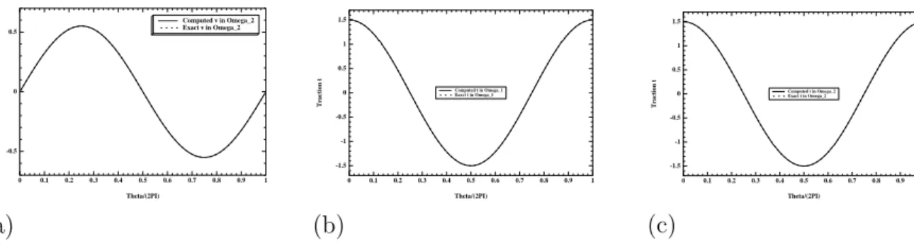
Theta/(2PI) v on Gamma_2 -1 -0.9 -0.8 -0.7 -0.6 -0.5 -0.4 -0.3 -0.2 -0.1 0 -0.3 -0.2 -0.1 0 0.1 0.2 0.3 Exact solution
Solution for theta=1 Solution for optimal Solution for dynamical 1 Solution for dynamical 2
(a) Theta/(2PI) t on Gamma_2 -1 -0.9 -0.8 -0.7 -0.6 -0.5 -0.4 -0.3 -0.2 -0.1 0 -1 0 1 -0.5 0.5 Exact solution Solution for theta=1 Solution for optimal Solution for dynamical 1 Solution for dynamical 2
(b) Theta/(2PI) s on Gamma_2 -1 -0.9 -0.8 -0.7 -0.6 -0.5 -0.4 -0.3 -0.2 -0.1 0 -1 0 1 -0.5 0.5 Exact solution Solution for theta=1 Solution for optimal Solution for dynamical 1 Solution for dynamical 2
(c)
Fig. 2.6 – Numerical and exact solutions for displacement v (a) and tractions t (b), s (c) for
N = 320 Theta/(2PI) u on Gamma_1 0 0.1 0.2 0.3 0.4 0.5 0.6 0.7 0.8 0.9 1 0 -0.5 0.5 p=1 p=2 Exact (a) Theta/(2PI) v on Gamma_1 0 0.1 0.2 0.3 0.4 0.5 0.6 0.7 0.8 0.9 1 0 -0.5 0.5 p=1 p=2 Exact (b) Theta/(2PI) u on Gamma_2 -1 -0.9 -0.8 -0.7 -0.6 -0.5 -0.4 -0.3 -0.2 -0.1 0 -0.3 -0.2 -0.1 0 0.1 0.2 0.3 Exact solution No-perturbation p=1 p=2 (c)
Fig. 2.7 – Perturbed displacements u (a), v (b) data on Γ1 and the corresponding numerical displacement u (c) results with N = 320
Noisy on the displacements data
We examine the algorithm stability when u and v data are noisy. The noisy data on displacements are presented in Fig. 2.7 (a), (b) and the corresponding numerical solutions are shown in Fig. 2.7 (c) and Fig. 2.8 (a).
Theta/(2PI) t on Gamma_2 -1 -0.9 -0.8 -0.7 -0.6 -0.5 -0.4 -0.3 -0.2 -0.1 0 -1 0 1 -0.5 0.5 Exact solution No-perturbation p=1 p=2 (a) Theta/(2PI) t on Gamma_1 0 0.1 0.2 0.3 0.4 0.5 0.6 0.7 0.8 0.9 1 -2 -1 0 1 2 p=1 p=2 Exact (b) Theta/(2PI) s on Gamma_1 0 0.1 0.2 0.3 0.4 0.5 0.6 0.7 0.8 0.9 1 -2 -1 0 1 2 p=1 p=2 Exact (c)
Fig. 2.8 – Numerical traction t (a) results with perturbed displacements data with N = 320 and perturbed tractions t (b), s (c) data on Γ1.
Tab. 2.2 – CPU time for different solvers (first iteration) for dynamical 1 N LU BI-CGSTAB CGNE CGNR CGR CGS 80 0.0579 0.0619(83) 0.0709(99) 0.0689(92) 0.1549(93) 0.0699(97) 160 0.4479 0.2899(75) 0.3239(101) 0.3239(94) 0.6499(77) 0.3549(98) 320 13.953 4.4043(83) 13.510(432) 7.7138(243) 13.053(89) 5.0732(93) 640 122.28 21.042(85) 85.438(611) 32.835(227) 50.697(78) 23.798(97) 1280 907.99 84.896(90) 1054.1(1964) 388.05(719) 221.24(85) 88.798(94)
Noisy on the tractions data
We examine the algorithm stability when t and s data are noisy. The noisy data on tractions are presented in Fig. 2.8 (b), (c) and the corresponding numerical solutions are shown in Fig. 2.9. Theta/(2PI) u on Gamma_2 -1 -0.9 -0.8 -0.7 -0.6 -0.5 -0.4 -0.3 -0.2 -0.1 0 -0.3 -0.2 -0.1 0 0.1 0.2 0.3 Exact solution No_perturbation p=1 p=2 Theta/(2PI) t on Gamma_2 -1 -0.9 -0.8 -0.7 -0.6 -0.5 -0.4 -0.3 -0.2 -0.1 0 -1 0 1 -0.5 0.5 Exact solution No_perturbation p=1 p=2
Fig. 2.9 – Numerical displacement u (left) traction t (right) results obtained for perturbed tractions data and N = 320.
For p ≥ 3, the numerical results obtained with perturbed data coincide with the numerical results obtained with no perturbed data. Therefore this case is not presented here.
It can be seen that as p increases, the numerical solution better approximates the exact solution, whilst remaining stable. For p = 1, the obtained results are to be considered more than reasonable, keeping in mind that the problem (2.5), (2.6) and (2.8), is an ill-posed problem with a very oscillatory data.
Comparison of LU decomposition and linear iterative solvers
To compare the efficiency for different iterative solvers, five computational meshes are used to generate five systems of 160, 320, 640, 1280, 2560 linear equations.
The iterative solvers BI-CGSTAB, CGNE, CGNR, CGR and CGS, are considered. Table 2-3 summarizes the results obtained for these solvers. The times shown are the average time in CPU times. The average number of iterative solver iterations is given in brackets. We used α = 10−07 as convergence tolerance in (2.31).
Tab. 2.3 – CPU time for different solvers (first iteration) for dynamical 2 N LU BI-CGSTAB CGNE CGNR CGR CGS 80 0.06 0.12(99 ;177) 0.15(98 ;163) 0.12(91 ;108) 0.28(89 ;84) 0.11(90 ;96) 160 0.47 0.61(79 ;237) 1.10(93 ;330) 0.66(93 ;146) 1.33(76 ;80) 0.64(86 ;106) 320 14.0 7.13(72 ;83) 19.1(305 ;297) 10.7(115 ;230) 18.2(72 ;58) 7.66(81 ;71) 640 122 29.2(68 ;55) 149(440 ;636) 50.4(88 ;267) 84.3(69 ;58) 36.5(77 ;75) 1280 913 129(69 ;87) 1117(718 ;1362) 448(120 ;712) 321(69 ;58) 137(73 ;61)
All the Krylov methods worked well, some, BI-CGSTAB and CGS, performed very well, yielding the solution in a small number of iterations. CGNE and CGNR revealed some difficulty in achieving a good convergence. The results show that BI-CGSTAB and CGS are more efficient than LU decomposition procedure, but BI-CGSTAB is by far the fast solver. The normalizing technique corresponding to the CGNE method is penalized due to the worsening of the condition number of their matrix relative to the condition number of the matrix of the original linear system.
2.2
A domain decomposition method for boundary
element approximations of the elasticity
equa-tions
2.2.1
Introduction
Domain decomposition ideas have been applied to a wide variety of problems. We could not hope to include all these techniques in this work. For an extensive survey of recent advances, we refer to the proceedings of the annual domain decomposition meetings see. http ://www.ddm.org. Domain decomposition algorithms is divided into two classes, those that use overlapping domains, which refer to as Schwarz methods, and those that use non-overlapping domains, which we refer to as substructuring.
Any domain decomposition method is based on the assumption that the given compu-tational domain Ω is decomposed into subdomains Ωi, i = 1, . . . , M, which may or may
not overlap. Next, the original problem can be reformulated upon each subdomain Ωi,
yielding a family of subproblems of reduced size that are coupled one to another through the values of the unknowns solution at subdomain interfaces. Fruitful references can be found in [37, 40].
A numerical study of elasticity equations by domain decomposition method combined with finite element method was treated in [9, 14, 23]. A symmetric boundary element analysis with domain decomposition is studied in [13, 36]. This combination was also used for biharmonic equation in two overlapping disks [2].
We have chosen to associate the Dirichlet-Neumann and Schwarz methods with the direct boundary element method. Indeed, it only requires the discretization of the boun-daries of the subdomains. This technique of coupling reduces the number of unknowns and the time of computing. It has been used successfully for semiconductors simulation [33].
We consider a linear elasticity material which occupies an open bounded domain Ω ⊂ R2, and assume that Ω is bounded by Γ = ∂Ω. We also assume that the boundary consists of two parts Γ = Γ1∪ Γ2 where Γ1 and Γ2 are not empty and Γ1∩ Γ2 = ∅ where Ω is not
necessarily circular or rectangular.
Let V = (u, v) the displacement vector and S = (t, s) the traction vector governed by the following linear elasticity problem
G∆u + G 1 − 2ν µ ∂2u ∂x2 + ∂2v ∂x∂y ¶ = 0 in Ω, G∆v + G 1 − 2ν µ ∂2u ∂x∂y + ∂2v ∂y2 ¶ = 0 in Ω u = ˜u, v = ˜v on Γ1 t = ˜t, s = ˜s on Γ2 (2.39)
are the prescribed quantities.
2.2.2
Domain decomposition techniques
In order to use domain decomposition to linear elasticity, we describe, in this section, Dirichlet-Neumann and Schwarz methods.
Dirichlet-Neumann substructuring method
We decompose Ω into two non-overlapping subdomains Ω1 and Ω2 such that
Ω = Ω1 ∪ Ω2, and denote by Γ12 = ∂Ω1 ∩ ∂Ω2 the common interface between Ω1
and Ω2. We can write this method as follows.
– Step 1. Specify an initial Λ0 = (λ0, β0) on interface Γ
12 and k = 0.
– Step 2. Solve the mixed well-posed direct problem G∆uk 1+ G 1 − 2ν µ ∂2uk 1 ∂x2 + ∂2vk 1 ∂x∂y ¶ = 0 in Ω1, G∆vk 1 + G 1 − 2ν µ ∂2uk 1 ∂x∂y + ∂2vk 1 ∂y2 ¶ = 0 in Ω1 uk 1 = ˜u, vk1 = ˜v on Γ1∩ ∂Ω1, tk1 = ˜t, sk1 = ˜s on Γ2∩ ∂Ω1, uk 1 = λk, v1k= βk on Γ12 (2.40)
to determine the traction Sk
1 = (tk1, sk1) on the interface Γ12.
– Step 3. Solve the mixed well-posed direct problem G∆uk 2+ G 1 − 2ν µ ∂2uk 2 ∂x2 + ∂2vk 2 ∂x∂y ¶ = 0 in Ω2, G∆vk 2 + G 1 − 2ν µ ∂2uk 2 ∂x∂y + ∂2vk 2 ∂y2 ¶ = 0 in Ω2 uk 2 = ˜u, vk2 = ˜v on Γ1∩ ∂Ω2, tk2 = ˜t, sk2 = ˜s on Γ2∩ ∂Ω2, tk 2 = −tk1, sk2 = −sk1 on Γ12 (2.41)
to determine the displacement Vk
2 = (uk2, v2k) on the interface Γ12.
– Step 4. Update Λk+1 = (λk+1, βk+1) on the interface Γ
12 by λk+1 = θuk
2 + (1 − θ)λk on Γ12, βk+1 = θv2k+ (1 − θ)βk on Γ12 (2.42)
– Step 5. Repeat step 2 from k ≥ 0 until a prescribed stopping criterion is satisfied. where θ is positive parameter. This algorithm establish the solution of elasticity equations of Problem 2.39 in Ω as a limit of sequence (uk
1, v1k, uk2, vk2).
For this algorithm the following stopping criterion is used max¡kλk+1− λkk
L2(Γ12), kβk+1− βkkL2(Γ12)
¢
< T ol, (2.43) where T ol is a prescribed tolerance.