Evaluation of a start-up through the signaling theory : Tesla case study

(1)

1

HEC Paris

Master II Grande Ecole - Finance

Evaluation of a start-up through the signaling theory:

Tesla case study

Professor: Patrick Legland

Student: Alessandro Frau S39624

(2)

2

Graphs:

Graph 1: key aspects for an investment decision………7

Graph 2: investment decision process………7

Graph 3: lognormal distribution………26

Graph 4: Tesla and S&P500 share price evolution………..………28

Graph 5: impact of new information on Tesla share price………..31

Graph 6: Mr Musk incremental borrowings (in red) by time period……….………44

Graph 7: regression line between number of employees and Tesla’s stock price………..49

Graph 8: Tesla stock price vs number of shares owned by insiders………..50

Graph 9: Tesla stock price vs number of shares owned by Tesla management………..50

Graph 10: Tesla stock price vs number of shares owned by institutional investors that have a seat on the board………..51

(5)

5

Tables:

Table 1: key issues in multiples approach...21

Table 2: VC method...22

Table 3: start-up target returns………...23

Table 4: actual return by segment of companies………...23

Table 5: Damodaran’s results………...30

Table 6: profit and loss statement………...33

Table 7: economic balance sheet………...34

Table 8: days of working capital………...35

Table 9: cash flow statement………...36

Table 10: theoretical impact of warrant ratchets on shareholding structure...38

Table 11: Tesla equity financing rounds pre-IPO………...39

Table 12: subscription of convertible notes by major shareholders………...40

Table 13: IPO proceeds………...41

Table 14: convertible bonds features………...42

Table 15: Mr Musk investment in Tesla………...43

Table 16: Tesla’s investors prior IPO………...47

Table 17: Tesla alliances………...48

Table 18: expected stock price by the market from convertible bonds………...53

Table 19: Tesla analysis of unlevered beta and cost of equity………...54

Table20: Tesla frequency of returns over S&P500 returns from IPO to third follow-on…...55

(6)

6

Abstract

Fundamental analysis does not explain all of the value of start-ups or young companies. This analysis proposes to utilize selected signals to have a more accurate and complete view of the value of start-ups and young companies. Tesla is used as an example of this.

The research is divided in two parts: (i) a review of the literature body and key methods concerning company valuations, both fundamental and signal-based, and (ii) a case study to apply the signals theory to Tesla.

In the first part, a review of the signals theory is complemented by an analysis of the valuation techniques used to value a company.

In the second part, a fundamental valuation of Tesla done by Damodaran is used as a starting point to demonstrate that some signals were to be taken into account to fully understand Tesla’s stock price since fundamental analysis alone justified only a portion of the company’s value.

(7)

7

Theory

1. Useful signals

In evaluating a start-up company standard valuation techniques only explain part of the company’s value. For this reason, I find it appropriate to add a new perspective to the valuation analysis: the signals a company and its stakeholders give to the market may be a good leading indicator of future company performance and, hence, stock prices.

Interpreting the signals and account for them in a valuation model appears a difficult exercise and probably not so “scientific” compared to a DCF, a trade multiple analysis or a transaction multiple analysis. Nevertheless, some signals like the equity investment of an entrepreneur, the number of employees or the investment in the company by officers are strong indicators and ought to be taken into account to have a full view of a company’s valuation.

For this thesis I interviewed Mr Boris Golden of Partech Ventures, a venture capitalist fund (‘VC’), and found his point of view about seed investments and financing extremely interesting. When Partech invests in early-stage companies a significant part of the due diligence is based on signals given by the entrepreneurs rather than on results which are not yet achieved. The investment decision process is based on both rational elements, a sort of check list for some specific requirements, and subjective assessments or intuitions based on signals and market knowledge. In particular, Graph 1 shows three important aspects which are taken into account in Partech’s investment decision: people, disruptive approach (product, business model) and market. Graph 2 shows a simplification of the investment decision process.

(8)

8

Both graphs are a rationalization of a much more complex process. However, they help understand at what level the signals are identified (Graph 1) and when they are used ( Graph 2). Signals can then be divided in soft signals, more linked to intuition and experience, and factual signals, more linked to the interpretation of facts. Many soft signals are linked to the management team: credibility, reputation, critic management (open vs defensive), investment in the project (time, money...). On the other side, factual signals are likely to be found in the product and the market: maturity of the idea related to the market, readiness of the market to accept it, market insights on the product quality, other VCs willingness to invest. Both soft and factual signals are then processed in a rational way to express the reasons that bring to the willingness to invest, or not, in a project.

In general, signals can be a strong tool to evaluate or give an insight on the future valuation of a start-up or a company with a short track record. In fact, if the definition of a start-start-up is that of a company with negative results, negative cash flows and a binary business that either works or fails, using classic valuation techniques such as multiples and DCF is most of times impossible because:

- There are no positive results to compare with the industry - Risk and the cost of capital are difficult to estimate - Growth is hard to measure in the long term

- The probability of success of the business is unclear at this early stage.

Clearly, the drawback of a valuation through signals is that most signals are qualitative and as such cannot be utilised quantitatively in deriving a clear-cut hard value of a business. Still, they are strong leading indicators of future company performance, as demonstrated by the following review of some of the most significant theories about early stages signal valuations.

A. Leland and Pyle theory on informational asymmetries, financial structure and financial intermediation (1977)

This work demonstrates that in equilibrium the entrepreneur's equity position in his project is related to the value of his project.

(9)

9

The work is based on the assumption of Akerlof (1970) and Spence (1973) that an equilibrium between supply and demand cannot be found if the information is asymmetric. In fact, as Akerlof demonstrates, while sellers know the quality of their cars, buyers cannot distinguish among them. Therefore, the market value will reflect the average car quality. The price for a good car will then be too low and the price for a bad car too high. Owners of good cars will not be willing to sell their cars at a discount and only bad cars will be sold. Following this negative spiral, the market value will continue to decrease because the average expected value of cars will continue to decrease.

The same concept is applicable to entrepreneurial projects: without a signal, only bad projects will be financed.

To avoid incurring in the negative spiral, and for good projects to be financed, an information transfer must occur. The work demonstrates how entrepreneurs can send signals to the market about the project quality. One such action is the willingness of the founder (or any person with inside information) to invest in the project. In particular, a firm’s value increases with the share of the firm held by the entrepreneur.

This finding is in contrast with Modigliani and Miller (1958) where the value of a firm is independent from its financial structure.

The entrepreneur will try to maximise his wealth based on (i) the financial structure of the firm, (ii) his equity in the firm, (iii) his holding of a market portfolio and (iv) risk free assets. The maximisation problem must satisfy the entrepreneur’s budget constraints. It is demonstrated that in equilibrium the entrepreneur's equity position in his project is related to the value of his project. In fact, if the implied value of the firm were higher than its actual value, external investors would receive less than the return expected for this type of project. On the other hand, if the implied value of the firm were lower, the opposite would be true.

Two theorems are then demonstrated:

- “THEOREM I. The equilibrium valuation function µ(α) is strictly increasing with α over the relevant domain, if and only if the entrepreneur's demand for equity in his project is normal”, where µ(α) is the firm’s value related to the entrepreneur’s share in the firm α

(10)

10

- “THEOREM II. In equilibrium with signalling by α, entrepreneurs with normal demands will make larger investments in their own projects than would be the case if they could costlessly communicate their true mean”.

So a high shareholding stake held by the entrepreneur is interpreted as a signal of a good project with α as a signal. At the same time, a welfare loss arises because if the markets were totally efficient, there would be no need for any signal – which has a cost, as in the case of the entrepreneurs investing in their projects - to be communicated to the market for a proper appreciation of the true value of the firm.

To conclude, Leland’s and Pyle’s works demonstrate rationally that the entrepreneur’s share in the firm is a strong signal for the project value. In the context of evaluating a start-up or a company with little track record, this theory appears very useful for external investors in selecting projects. The fact that the entrepreneur believes in his own project and is aligned with external investors by risking a significant part of his wealth has to be interpreted as a strong signal about the project’s quality.

B. Signalling through inter-organizational relationships (Reuer, Tong and Wu, 2012)

This work demonstrates how a firm’s inter-organizational relationships (e.g. associations with prominent investment banks, venture capitalists and alliance partners) can send a signal about its value to the market. In particular, it analyzes the impact of these relations on the premium paid by acquirers on firms that had been listed in the last five years prior to the acquisitions.

Firms going through an IPO, like start-ups, have short track records and are subject to information asymmetries during the valuation process. Therefore, they will be subject to discounts, unless signals about their quality can be sent to the market.

According to this work, (e.g., Stuart et al., 1999; Hallen, 2008; Hsu, 2006) such signals as partnering with a leading investment bank for the underwriting, being backed by prominent venture capitalists or having strategic alliances all result in strong signals that have long-term effects on the value of start-ups:

(11)

11

- Partnering with a leading investment bank: there is a mutual benefit for a good firm to be sponsored by a leading bank and for a leading bank to sponsor a good firm. High quality firms should be willing to pay more for the services of reputable banks to use the bank’s reputation to lower the discount investors will pay. On the other hand, since banks repeat their offer to different clients, reputation is key and any opportunistic behaviour can affect future business. As a consequence, the most prominent banks will try to protect their reputation by minimizing the risk of sponsoring a bad company. This two-sided relationship is costly to replicate and therefore it increases the signalling value

- Being backed by a prominent venture capitalist: many firms are sponsored by a bank, but only few partner with a VC. The rationale for being backed by a VC can be similar to the one for partnering with a leading bank. However, having the support of a VC is an even stronger signal sent to the market in the sense that VCs have longer term views of a firm. VCs act in the middle between the firm and the market, because VCs are very selective and only chose the projects with the higher chances of success. VCs do not only put their reputation at stake, as banks do, but also money. So they track their investments, they bring their expertise to grow the companies and take a long term view. As for banks, associations with prominent VCs are costly to replicate, because private companies will need to accept a lower valuation when deciding to use a prominent VC’s reputation (Hsu, 2004), and high-quality projects are more likely to be able to bear such a cost

- Having strategic alliances: alliance partners will have an operational view that neither banks nor VCs have about a firm’s technologies and resources. As being associated with a leading bank or a prominent VC, having strategic alliances gives the firm the opportunity to use the partner’s reputation to convey a signal to the market about the true value of the project. The work tests the hypothesis that the acquisition premium is: (i) positively related to the reputation of the investment bank used for the IPO; (ii) is greater for targets backed by prominent VCs; and (iii) is positively related to the number of alliances the company has formed with prominent partners. The results are noteworthy because they confirm that these signals are significant to explain higher premia:

(12)

12

- Acquisition targets that were sponsored by banks with an above the median reputation during their IPO achieved an average premium of 51%, compared with an average of 43%, and a significance of p-value = 0.10 and t = 1.89

- Acquisition targets backed by prominent VCs achieved an average premium of 53%, compared with an average of 42%, with a significance of p-value = 0.01 and t = 2.64

- Acquisition targets that developed strategic alliances in the last five years achieved an average premium of 56%, compared with an average of 40%, with a significance of p-value = 0.001 and t = 3.63.

In conclusion, partnering with a leading bank, prominent VCs and strategic allies gives a strong signal to the market about a firm’s quality. This research is particularly important in the context of a start-up that, like IPO companies, has a short track record. Banks, VCs and allies will be willing to offer their reputation to firms with a short track record only if their perceived gains are higher than their risks: these partnerships are clearly a strong signal to the market.

C. Headcount growth as a signal for changes in valuation (Davila, Foster and Gupta, 2002)

This work tries to understand the relationship between growth in the number of employees and VC funding. In particular, one of the findings is that headcount impacts the valuation of the equity and that the growth in headcount is positively and significantly correlated to the growth in equity value. Headcount growth can be a signal about the quality of a firm because (i) it is a cost that only good firms are willing and able to bare and (ii) it shows increasing commitment in the project. Considered as a signal, headcount growth can be viewed as a real time measure of the firm. In fact, the research finds that the coefficient for growth in the number of employees is positive and significant at a 3.5% level suggesting a positive relationship between changes in equity value and changes in the number of employees.

(13)

13

In conclusion, it is interesting to note how the growth in headcount can be a significant signal about the quality of a start-up and on its equity value. Furthermore, headcount is easy to measure and gives an internal perspective about the quality of a firm.

D. Deducting information from insiders’ trades (Jeng, Metrick, and Zeckhause, 2003; Nejat Seyhun, 2000; Nejat Seyhun, 1986; Finnerty 1976; Lin and Howe 1990; Zaman 1988)

Many papers tried to answer two key questions regarding insiders’ trade analysis: the first is whether insiders earn abnormal returns and the second is whether outside investors can mimic insiders’ strategies to earn abnormal returns.

The findings of Jeng, Metrick, and Zeckhause (2003) are extremely important to understand the signals that insiders send to the market. In their work, two distinctive six-months portfolios were built, a purchase and a sale one, to track their performance against the market. Three methods are used to compare the results, the CAPM, the four factors model and characteristic-selectivity method. All three methods find that significant abnormal returns are earned by the purchase portfolio: this evidence suggests that insiders have a good feeling about the near-term development of their firm. On the other hand, none of the methods finds significant abnormal returns for the sale portfolio. The findings about the purchase portfolio work against the strong form of market efficiency and also show that the insiders’ position within the firm as well as the size of the firm have no impact on abnormal returns.

On the other hand, the insiders’ sale portfolio does not earn significant abnormal results. In fact, the insiders transactions might be motivated by other reasons than returns, like diversification purposes, rebalancing objectives or liquidity needs, that do not bring any relevant information.

Finnerty (1976) shows how insiders time the market using private information. According to this research, there is a relationship between insiders’ trades and future financial and accounting information. In particular, it is shown how insiders are long on small, high earnings and high dividends firms and short on large, low earnings and low dividends firms.

(14)

14

Lin and Howe (1990) confirm the previous studies and add that insiders are able to time the market so that insiders’ transactions have a significant predictive content.

These studies on insiders’ trading are extremely interesting because they confirm statistically that insiders’ trades bring information about future results and that insiders can earn abnormal profits. Now, concerning the second question, whether outsiders can earn abnormal results by following insiders’ strategies, Lin and Howe (1990), Rozeff and Zaman (1988) and Seyhun (1986), demonstrate that outsiders are not able to gain from insiders’ informative trades. In fact, actively trading on the information provided by insiders’ is subject to trading costs that completely offsets the abnormal returns otherwise gained.

The results are interesting because, even if actively mimicking insiders’ strategies does not bring any abnormal return, it is demonstrated that insiders’ positions are informative about future performance and, hence, company values.

2. Fundamental analysis

Fundamental analysis - like DCF and multiple approaches - are typically the starting point when evaluating a company. They are supposed to be scientific because they force the analyst to understand the firm by building a sound model that forecasts a firm’s future performance and they benchmark a firm to the market for a consistent approach.

However, they have many limitations for companies that: - Have negative results and operating margins - An unpredictable cost of capital

- An unpredictable growth.

All these elements are typical of a start-up or a young company with little track record and little visibility about its future returns. To arrive at a solid valuation of a start-up is normally quite difficult for three main reasons: (i) past accounting data are unavailable and not significant for fast growing

(15)

15

companies, (ii) projections are mostly subjective, and (iii) valuations are done occasionally at each round of financing.

Therefore, even if fundamental analysis has many benefits, they are best applied to mature companies with a reliable visibility about their future performance. Follows a brief overview of the main fundamental techniques with their pros and cons.

A. DCF

The model

As Damodaran says, “Every asset that has an intrinsic value that reflects its cash flow potential and its risk”.

The idea is that every asset class can be valued based on two factors: (i) future cash flows and (ii) the cost of capital that reflects the risk of the project, as follows:

Therefore, the value of any project is the sum of its future cash flow discounted by the cost of capital. The asset quality depends on different variables that may influence cash flows like:

- The size - The time - The duration - The risk.

The starting point of a DCF is a company’s business plan. A top down approach is often used to estimate available cash flows and projections are done over a time horizon to estimate future cash

(16)

16

flows based on assumptions on sales growth, margins, CAPEX investments and working capital requirements. Usually hypotheses are made to estimate the aggregates over a 10-year horizon and a terminal value is then calculated to account all the future cash flows from year 10 onward. This model has the advantage in that it forces the analysts to understand the business to make assumptions about the future, but it is obviously better suited for mature companies with relatively stable and predictable cash flows.

Two main methods are used to estimate the terminal value: (i) the growing perpetuity formula

where r is the discount rate and g the growth rate, usually set as the GDP growth rate, and

(ii) the multiples approach where current multiples are applied to the projected aggregates of Sales, EBITDA or EBIT.

All the cash flows available to repay debt holders and equity holders are discounted by the weighted average cost of capital (WACC), which is a weighted average of the cost of the equity and the debt, as follows:

- Ke is the cost of equity or required return demanded by shareholders to invest in a firm

- Kd is the cost of the debt of a firm, net of taxes, also to account for the tax shield coming from

an increase in debt

- t is the marginal tax rate of the firm

- E is the market value of a company’s equity - V is the market value of a company’s debt.

The Ke is a measure of the riskiness of an asset. The higher the risk, the higher the required rate the

investor will ask to invest in a project. There are different ways to estimate the cost of capital, however the most broadly used is the capital asset pricing model (CAPM) developed by Sharpe (1964) and Lintner (1965) based on the work of Markowitz on diversification and portfolio theory.

The model says that the cost of equity is equal to a risk-free asset plus a premium based on the stock risk and the systemic risk, as follows:

(17)

17

where Rf represents the return of risk free assets, Rm the market return and β the systemic risk of a

stock given by where Ri are the returns of an asset and Rm the returns of the market

portfolio.

Once the cash flows and the terminal value are estimated, they are discounted by the WACC to obtain the enterprise value (EV), or the intrinsic value available to debt holders first and shareholders thereafter. To obtain the equity value, or the value available to shareholders, net debt is subtracted from the EV, as follows:

Pros

The real benefit of a DCF is that it gives a rational framework to analyze a company. According to Damodaran every asset class can be valued with a DCF because of the possibility to estimate future results.

Another benefit of the model is that it makes the analyst focus about the many drivers of a company that may have been otherwise overlooked. Estimating the future sales growth, the margins, the investments and the working capital required to run a business helps having a clear view about a company.

Moreover, the model is one of the most scientific ways to look at a company and give a good approximation of the true firm value when its cash flows are easily foreseeable, typically in mature firms or project finance companies.

(18)

18

Cons

On the other hand, the DCF is also subject to many flaws that are amplified for start-ups.

The first problem is about the credibility of the business plan. The entire model is based on the business plan, so having differences with the reality can have a strong impact on the final valuation. In general, business plans tend to be overoptimistic about the future, thus overvaluing a company. For start-ups the problem could even be that a business plan is impossible to build, given that future performance is impossible to forecast. This problem is particularly true for start-ups or young companies that operate in sectors with no competitors, where the company itself is creating the demand. In fact, if it is difficult to know what will be the demand for a product or a service, it could be impossible to feed the DCF model with the data required.

The second problem is the weight of the terminal value over the overall value. The problem of the terminal value is that it is placed far in time, usually 10 years from the first cash flow, so it is particularly uncertain. If most of the valuation comes from the terminal value, most of the valuation will be subject to an acute realization risk. This risk is lower for predictable cash flows, typically initial cash flows. This problem is exacerbated for start-ups, where the terminal value may exceed 100% of the total valuation. In fact, a start-up or a young company typically has an initial period with negative cash flows that become positive only later on.

The third problem of the DCF is the discount factor. The discount factor is the single variable that has the highest impact on the total valuation: a small change in the discount factor can have a huge impact on the final value. This problem becomes even more significant for a start-up or a young company. In particular, two reasons make the discount factor difficult to assess for a start-up: (i) it is extremely hard to evaluate the risk of a company that is creating its market or that it does not have any peers to compare with, and (ii) the discount factor tends to change over the years, usually decreasing over time, because the venture risk decreases given a longer track record and a higher visibility over future results.

(19)

19

The fourth problem relies on the capacity of an asset to generate cash flows. The DCF method evaluates the cash flows generated by existing assets andby future assets as well as the increased efficiency of existing assets. The problem is that no one knows for sure: (i) the level of future investments and (ii) the future improvements of existing assets. This problem is even more amplified for start-ups or young companies, where present assets are extremely low, thus most of value comes from “growth assets” or future assets.

Extension of the DCF model to start-ups by Damodaran

Damodaran in his article “Valuing Young Growth Companies”, gives a six-step model to evaluate fundamentally a young company, trying to apply it to LinkedIn in occasion of its IPO in 2011.

The six steps are as follows:

- Estimate revenues by calculating the size of the market and what share the company will gain - Estimate the margins. Damodaran suggests to set a target margin and estimate how difficult it

will be to reach that target over time

- Assess the required reinvestment to sustain growth as needed

- Estimate the cost of equity and capital over time. Damodaran takes sector averages to calculate betas, cost of debt and debt-to-equity ratios focusing on the riskiest and the smallest companies for the initial phase and on more mature companies for later phases

- Estimate the expected value and adjust for the risk of failure. The start-up growth period should end at a certain point to reach a growth level more in line with a mature business. Also some other aspects should be taken into consideration in assessing whether a firm may survive: (i) its flexibility in raising funding, (ii) its dependence on some few key employees, and (iii) market conditions

(20)

20

Applying this modified version of the DCF to LinkedIn’s IPO, Damodaran tried to obtain a fundamental value for a young company with very little track record. However, his resulting final valuation of $23.27 per share is far away from the opening price of $43 and its continued growth.

In conclusion, even this new DCF model for young companies is not in a position to value start-ups: therefore, either the market is remote from fundamentals or fundamental methods have some limits in explaining start-ups’ or young companies’ intrinsic value.

B. Multiples approach

The model

There are two categories of multiples: (i) trade multiples or multiples of comparable listed companies, and (ii) past transaction multiples. Each category is divided in: (i) indirect multiples that calculate first the enterprise value (EV) and then the equity value by subtracting the net debt from the EV, or (ii)

direct multiples that calculate directly the equity value of a company.

An average or a mean of comparable multiples is usually used and multiplied by the company’s aggregate figures (e.g. Sales, EBITDA, EBIT, Net Income) to obtain the enterprise value in the case of indirect multiple or the equity value in the case of a direct multiple. Whenever possible, a number of multiples is used to build a valuation range.

The limitations

Using the multiples method can be extremely easy and logical since it is quite rational that the value of a firm falls within a range given by comparable firms or transactions in the market. However, using the multiples approach can be misleading. The underlying assumption of using comparable multiples

(21)

21

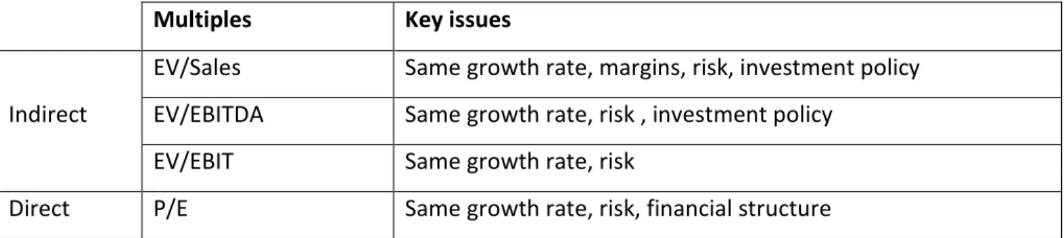
is that aggregates such as EBITDA, EBIT or Earning are positive. Table 1 tries to give an overview of the most common issues:

Multiples Key issues

Indirect

EV/Sales Same growth rate, margins, risk, investment policy

EV/EBITDA Same growth rate, risk , investment policy

EV/EBIT Same growth rate, risk

Direct P/E Same growth rate, risk, financial structure

Table 1: key issues in multiples approach

Common to all multiples are the growth rate and the company’s risk. To be comparable two firms need to have the same expected growth. In fact, from the company’s sales depend the cash flows, earnings and dividends, all key aspects in establishing the intrinsic quality of a company. The same is true in evaluating risk. It does not make sense to compare companies with different risk profiles based on quality and quantity of earnings.

The growth rate and the risk are important factors that potentially limit the use of multiples. In fact, it can be very difficult to find comparables with the same growth profile, at the same development maturity and subject to the same external and internal risks. However, even though these two limits can have a strong impact on the valuation of a company, sometimes comparables are still used to have a broad view of values.

Another factor that must be taken into account when using multiples is the investment policy: investments affect present and future cash flows, but also the profitability of a company.

Another factor, that strongly limits the use of the P/E ratio, is the financial structure. By using the ratio of a comparable company, it is assumed that the two companies share the same financial structure. If this is not the case, this ratio can be extremely misleading. For example, applying a P/E ratio of 15 to the earnings of a company that has net cash of 100 invested at 4% after tax, would be the same as valuing the capital employed at 15 times EBIT after tax and at 15 times the financial income after tax (or 15x4%x100 = 60). This means that the cash worth 100 will be undervalued by 40 (100-60).

(22)

22

3. Venture capitalist (VC) method

The VC method has the benefit of being easy and fast to implement giving a view on what VCs expect from a start-up.

Two complementary approaches are proposed: (i) the first being more to discriminate among possible investments and (ii) the second being more schematic.

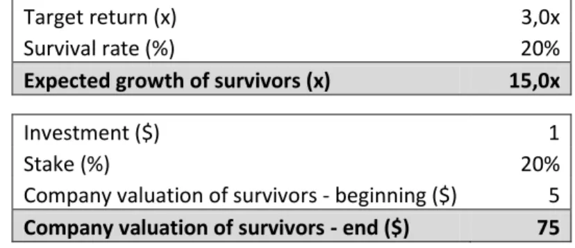
For the first method, the VC sets a target return for its portfolio of investments (usually 2x to 3x cash-on-cash over five years). Given the target return and an expected survival rate of the portfolio’s companies, the VC knows the expected growth of the companies it has to invest in, as follows:

For example, if a VC’s target return is 3x and the survival rate is 20%, the VC has to invest in companies with an expected growth of 15x. Therefore, it can also assume the revenues expected by the portfolio companies. Assuming that one unit of enterprise value equals one unit of sales and that the VC acquires 20% of the target companies, the sales the VC expects from its portfolio companies are given by the following formula:

Therefore, assuming an investment of $1, the VC expects to invest in companies that have target sales of $75.

The logical steps are summarized by Table 2.

Target return (x) 3,0x

Survival rate (%) 20%

Expected growth of survivors (x) 15,0x

Investment ($) 1

Stake (%) 20%

Company valuation of survivors - beginning ($) 5

Company valuation of survivors - end ($) 75

(23)

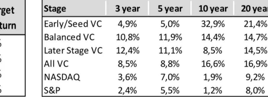
23 Stage of development Typical target rates of return Start up 50-70% First stage 40-60% Second stage 35-50% Bridge / IPO 25-35%

Stage 3 year 5 year 10 year 20 year

Early/Seed VC 4,9% 5,0% 32,9% 21,4% Balanced VC 10,8% 11,9% 14,4% 14,7% Later Stage VC 12,4% 11,1% 8,5% 14,5% All VC 8,5% 8,8% 16,6% 16,9% NASDAQ 3,6% 7,0% 1,9% 9,2% S&P 2,4% 5,5% 1,2% 8,0%

The second more schematic approach is a four-step process proposed by Damodaran: - Estimate expected earnings for the near future, normally two to five years

- Obtain the value of the company at the end of the forecast period. Multiples of comparable listed companies or of transactions of companies operating in a similar business are used to arrive at the company’s value

- Discount the value of the company at the end of the forecast period. As shown by Damodaran (Tables 3 and 4), the discount rates are much higher than the actual returns of VCs. The gap is explained by the failure risk that is factored in the discount rates, as follows:

Source: The dark side of valuation, Damadoran (2009)

- Calculate the share of the firm the VC is entitled to based on its contribution, with the post money valuation = pre money + new capital, as follows:

Unfortunately, also the VC method has several flows. Damodaran in particular finds that four problems may arise:

- The method encourages “game playing” or bargaining on the value of the firm. The method is not based on a real analysis of the company, but more on the target revenues or project earnings proposed by the founders and the VCs to respectively bring up or down the value of

(24)

24

the firm. Consequently, the firm’s value becomes the bargaining base between the founders and the VCs

- The method has the benefit of being easy and quick to use, however the comparable multiples method does not consider the future cash flows, whereas the multiple of the firm at the end of the period will be a function of the cash flow generation ability

- The assessment of the discount rate has two main problems. The first is that there is a discrepancy in using a cost of equity when discounting an enterprise value derived from a multiple of sales: the cost of capital should be used instead. The second is that factoring in the probability that the firm will not survive implies that the rate will not change over time

- In adding the new capital to the pre-money valuation to calculate the share of the VC in the firm, it is assumed that the money raised stays within the firm to fund future investments. If part of the new money is used to buy out existing shareholders, the money that goes out of the firm should not be added to the pre-money valuation.

4. Real option valuation

The real option valuation technique sees the value of a firm as a call option held by shareholders, as if the shareholders at a certain time had the possibility either to buy the residual value of their company after having paid all liabilities or leave the company. This valuation technique looks particularly suited for start-ups because, as Kotova (2014) says, it is appropriate for projects that:

- Have a high level of uncertainty

- Have flexible decision making processes

- Have financial results mostly dependent on intangible assets that have yet to prove their ability to generate results.

The valuation is based on the following Black-Scholes (1973) model:

(25)

25

where:

- Ve is the equity value of a company

- S is the enterprise value calculated as the present value of future cash flows

- K is the option exercise price or the value of investments required for the project’s implementation

- r is the risk-free rate

- is the time to maturity

-  is the volatility

- N is the cumulative distribution function of a normal centred variable and where: - -

As Kotova (2014) points out: “the price of the option is higher when the present value of expected cash flows grows, the cost of project implementation is lower, there is more time before the expiry of the option [and the project is subject to a] greater risk”.

The biggest challenge of using the real option model relies in the difficulty of finding reliable data to

calculate 

Some argue that there could be two major concerns in using the Black-Scholes model to value privately held companies and in particular start-ups:

- There should be a non-tradability discount on the option

- There is a an understatement of the volatility when using lognormal returns. However, none of these concerns has a real impact on the model.

For the first, it is argued there should be no discount applied to the option because the non-tradability discount should already be incorporated in the asset.

(26)

26

For the second, as explained by Metrick and Yasuda (2010) in ‘Venture Capital and the Finance of Innovation’, “the objection here is usually caused by confusion about the difference between normal distributions (which look like a bell curve when drawn in periodic returns) and lognormal distributions (which look like a bell curve if drawn in log returns, but look like Graph 3 if drawn in periodic returns)”.

Graph 3: lognormal distribution

(27)

27

Case study: Tesla

In this section, a case study is developed to gauge the implications of the signal theory on the valuation of Tesla, a young listed company that still has negative cash flows, negative results and its business model is based on the disruptive idea to sell only electric cars.

As discussed with Mr Boris Golden of Partech Ventures, companies at a very early stage are extremely hard to valuate because entrepreneurs are selling a very unproven project to VCs with very limited track records and results. VCs are able to estimate what percentage of a start-up it is reasonable to acquire thanks to a due diligence process that, among others, takes into consideration the soft and factual signals previously discussed such as the pressure that comes from other investors. At more advanced maturity stages, companies start to have a track record, the chance to fail diminishes and more scientific approaches can be used.

The starting point of this analysis will be the conclusions reached by Damodaran on his fundamental valuation of Tesla which comes far short of Tesla’s market value. The signal theory will then be used to try to explain the gap between Damodaran’s valuation and the stock market valuation.

1. Adding to Damodaran fundamental analysis

In his paper (2014) “Tesla: Anatomy of a Run-up Value Creation or Investor Sentiment?” Damodaran demonstrates how Tesla is fundamentally overvalued after the sevenfold stock increase from March 2013 to February 2014, as shown in Graph 4.

Damodaran argues that Tesla “operates in an industry automotive manufacturing, and a potential industry, battery construction, that are mature and are populated by established competitors” so a DCF anchored on established fundamentals should be appropriate.

(28)

28

Damodaran’s conclusion is that Tesla’s stock price, according to his fundamental analysis, is overvalued by approximately 150% and that the market value and the rational value can diverge for prolonged periods of time.

Graph 4: Tesla and S&P500 share price evolution

Source: Bloomberg

Damodaran, based on DeLong, Shleifer, Summers and Waldman (1990), concludes that Tesla’s share price is based on investors sentiment that is defined “as a belief about future cash flows and investment risks that is not justified by the facts at hand”.

According to the paper, there are five reasons supporting the soundness of a fundamental analysis on Tesla:

- Tesla is part of a mature industry where the long term growth rate corresponds to the GDP growth rate. So there should not the problem of making assumptions over the long term growth of the company

- The mature state of the industry makes it easy to find comparables and a comparable analysis is useful to have a sense of a company valuation

- The technology is known and innovations are incremental. Therefore, there is not the problem of having much of the value coming from a disruptive technology

22/03/2013 26/02/2014 0 50 100 150 200 250 300 29/06/2010 29/12/2010 29/06/2011 29/12/2011 29/06/2012 29/12/2012 29/06/2013 29/12/2013 29/06/2014 29/12/2014

Tesla Share Price S&P Price (rebased)

+752%

+92% +591%

+19%

(29)

29

- The stable nature of the industry should not make the expected return, thus the discount rate, changing rapidly

- The stock increase happens over one year, therefore it cannot be related to the market learning previously undisclosed information.

The analysis is made in three steps: (i) a DCF valuation, (ii) an analysis of the new information and (iii) an analysis of the impact of noise trading on Tesla’s stock price.

While the results provided by Damodaran to demonstrate that Tesla’s stock is fundamentally overpriced seem conclusive, these result will be the starting point of this case study to show how some signals must be considered to have a full picture of the stock price increase.

A. DCF valuation

The model used is the one presented earlier adjusted to value young companies.

- Forecasting the revenue growth rate. This estimate is driven by the market average and the intrinsic quality of the company. The model estimates an annual growth rate over 10 years of 70%, making Tesla at the end of year 10 a major player in the automotive industry

- Forecasting operating margins. Tesla’s operating margins were very negative till the introduction of Model S. With Model S a turnaround of the company happened, but margins were still negative. The valuation model expects Tesla will be able to reach Porsche’s profitability, one of highest in the market, of 12.5%

- Estimating the investment required to achieve the growth rate and operating margins. The ratio taken into account is sales/capital and till the last quarter of 2013 it has been lower than one, even if it has been increasing. This means that the company was not able to convert its investments in sales. From the first quarter 2014 the valuation model considers the industry average

(30)

30

- Estimating the cost of capital adjusted for the chance of failure. The model is optimistic about the probability of failure, set at zero, and estimates that the cost of capital will be decreasing converging to the market average of 8%

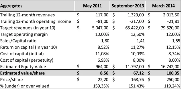
As Table 5 shows, Damodaran’s valuation results as of September 2013 and March 2014 arrive at much lower fundamental values for Tesla than the market does.

Table 3: Damodaran’s results

Source: Tesla: Anatomy of a Run-Up, Cornell and Damodaran (2014)

B. Impact of new information

Damodaran then tries to explain rationally the sevenfold increase by an event analysis. Graph 5 summarizes the major events identified.

Aggregates May 2011 September 2013 March 2014

Trailing 12-month revenues $ 117,00 $ 1.329,00 $ 2.013,50 Trailing 12-month operating income $ -81,00 $ -217,00 $ -21,81 Target revenues (in year 10) $ 5.047,00 $ 65.422,00 $ 79.520,00

Target operating margin 10,00% 12,50% 12,00%

Sales/Capital ratio 1,80 1,41 1,55

Return on capital (in year 10) 8,52% 11,27% 12,15%

Cost of capital (initial) 11,08% 10,03% 8,74%

Cost of capital (perpetuity) 6,93% 8,00% 8,00%

Estimated Equity Value $ 964,00 $ 11.797,00 $ 16.742,00

Estimated value/share $ 8,56 $ 67,12 $ 100,35

Price/share $ 22,20 $ 168,76 $ 250,00

(31)

31 Graph 5: impact of new information on Tesla share price

Sources: Bloomberg and Cornell and Damodaran (2014)

To start, the event analysis concentrates on earnings surprise and the stock price reaction. Three quarters bring positive news and one negative results. According to the paper, earning surprise explains 24% of residual returns (Tesla returns minus S&P500 returns).

The second step was to study other news that could fundamentally explain the price run-up. It is demonstrated how little real information came to the market that could explain such a price increase. The news are separated in two groups, one associated with positive and the other with negative residuals. Of the positive, 16 are not related to earnings announcements. Of those, only three contain fundamental information: two about anticipated higher sales and one about the planned introduction of a mass market car in 2015. Three others are related to positive analyst reports, however they do not contain any new fundamental information and the others are meaningless information where most of the times the information has been the increase in stock price itself. On the negative side, seven residuals were not related to earnings. Of those, four were not related to meaningful information, two related to fires involving Model S and one related to a negative broker’s report. In conclusion, according to the paper, the event analysis fails to explain fundamentally the increase in stock price. 0 50 100 150 200 250 300 22/03/2013 22/05/2013 22/07/2013 22/09/2013 22/11/2013 22/01/2014

Tesla Share Price

21 Positives 8 Negatives +13.9%: MS Report +8.4%: Positive results +5.4%: Q4 results +15.7%: Higher deliveries +5.6%: Mass market car announced +16.5%: MS top pick -10.2%: Investigation on reporting rules -7.5%: Third fire -14.5%: Q3 results +8.0%: Agreement with Panansonic -6.2%: First fire +6.2%: Safest car tested in US +14.3%: Q2 results +10.3%: CNN article -14.3%: GS bearish report +9.1%: Jefferies doubles target price to $130 -6.9%: Forbes bearish article +13.6%: Bloomberg article +6.3%: Repaym ent of DOE loan +8.7%: Follow-on +14.4%: CNN article +10.6%: FT article +24.4%: Q1 results -6.7%: CNN article +9.1%: Change in guarantee +7.3%: Service program an.cmt +5.3%: CNN article -7.3%: leasing program +15.9%: First profit Quarter results Corporate news $

(32)

32

C. Impact of noise trading

Damodaran’s paper concludes the analysis trying to assess the impact of noise traders on the stock price increase with the use of two measures: (i) the percentage ownership of institutional investors and (ii) the ratio of shares sold short to the shares outstanding.

For the first measure, it is shown how the institutional ownership peaks at 87% just as the run-up begins and steadily declines to approximately 65% at the end of the run-up. This finding supports the noise trading theory for which “smart” institutional investors liquidate their positions when the stock price is far from its fundamental value. However, also Damodaran says that “the evidence is far from overwhelming”; in fact, at the end of the run-up institutional investors still account for more than two third of Tesla shareholdings.

For the second measure, it is shown how short positions plummeted at the beginning of the run-up and increased again when the stock price passed the $150 mark. The first drop in short positions, according to the paper, is in line with the noise trading theory for which short sellers acknowledge the increased volatility of the stock when the run-up begins, thus they “are unwilling to keep their short position in the face of higher perceived volatility”. However, when the stock price passed $150, short sellers again started to short the stock. According to theory this is rational if short sellers perceive that the fundamental value is lower than the stock price. In fact, the higher perceived risk would be offset by an increased expected return.

Only part of the increase in stock price could be explained by noise traders, in fact institutional shareholders were net sellers and short positions rose. However, how Damodaran says, “the magnitude of these offsetting effects was too weak to blunt the sevenfold increase in the price”. Damodaran concludes by saying that “investor sentiment must at least be part of the story” and that “at some point, as the information about the cash flow generating characteristics of the business become clearer, price and value should start to converge”, i.e. markets are crazy and I will be right in the long run!

(33)

33

2. Financial analysis

Before entering into details of how signals should be used to have a complete vision about Tesla’s value, Tables 6, 7, 8 and 9 summarise Tesla’s figures.

Table 4: profit and loss statement

Sources: Tesla annual reports

Profit and loss statement

As of 31/12 in % of sales 2010A 2011A 2012A 2013A 2014A

Sales 100% 100% 100% 100% 100% Cost of sales 74% 70% 93% 77% 72% Gross margin 26% 30% 7% 23% 28% R&D 80% 102% 66% 12% 15% SG&A 72% 51% 36% 14% 19% EBITDA (117%) (115%) (88%) 3% 4% D&A 9% 8% 7% 6% 9% EBIT (126%) (123%) (95%) (3%) (6%) Financial income (1%) 0% 0% (2%) (3%)

Other income (expense) (6%) (1%) (0%) 1% 0%

Pre-tax income (132%) (124%) (96%) (4%) (9%)

Corporate income tax 0% 0% 0% 0% 0%

Net income (group's share) (132%) (125%) (96%) (4%) (9%)

Profit and loss statement

As of 31/12 in '000 2010A 2011A 2012A 2013A 2014A

Sales 116.744 204.242 413.256 2.013.496 3.198.356 Cost of sales 86.013 142.647 383.189 1.557.234 2.316.685 Gross margin 30.731 61.595 30.067 456.262 881.671 R&D 92.996 208.981 273.978 231.976 464.700 SG&A 84.573 104.102 150.372 285.569 603.660 EBITDA (136.215) (234.569) (365.458) 53.943 114.976 D&A 10.623 16.919 28.825 115.226 301.665 EBIT (146.838) (251.488) (394.283) (61.283) (186.689) Financial income (734) 212 34 (32.745) (99.760)

Other income (expense) (6.583) (2.646) (1.828) 22.602 1.813

Pre-tax income (154.155) (253.922) (396.077) (71.426) (284.636)

Corporate income tax 173 489 136 2.588 9.404

(34)

34

Table 6 shows the profit and loss aggregates. It is interesting to note that the company has always had negative results, but 2013 represents a turning point with the positive impact of the introduction of Model S. Sales skyrocketed by about 5x and EBITDA started to be positive. Also, net income increased dramatically in 2013: if before 2013 1$ in sales produced a loss of approximately 1$, after 2013 1$ in sales produced no more than 0.1$ of losses.

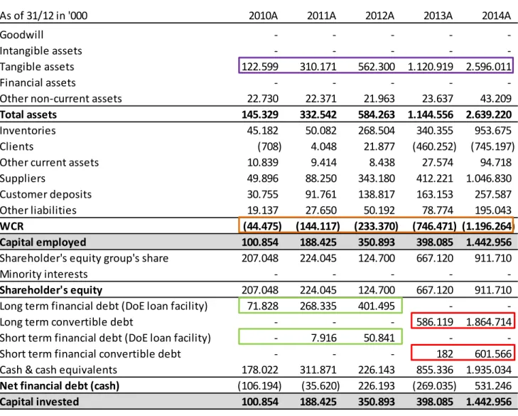
Table 5: economic balance sheet

Economic balance sheet

As of 31/12 in '000 2010A 2011A 2012A 2013A 2014A

Goodwill - - - -

-Intangible assets - - - -

-Tangible assets 122.599 310.171 562.300 1.120.919 2.596.011

Financial assets - - - -

-Other non-current assets 22.730 22.371 21.963 23.637 43.209

Total assets 145.329 332.542 584.263 1.144.556 2.639.220

Inventories 45.182 50.082 268.504 340.355 953.675

Clients (708) 4.048 21.877 (460.252) (745.197)

Other current assets 10.839 9.414 8.438 27.574 94.718

Suppliers 49.896 88.250 343.180 412.221 1.046.830

Customer deposits 30.755 91.761 138.817 163.153 257.587

Other liabilities 19.137 27.650 50.192 78.774 195.043

WCR (44.475) (144.117) (233.370) (746.471) (1.196.264)

Capital employed 100.854 188.425 350.893 398.085 1.442.956

Shareholder's equity group's share 207.048 224.045 124.700 667.120 911.710

Minority interests - - - -

-Shareholder's equity 207.048 224.045 124.700 667.120 911.710

Long term financial debt (DoE loan facility) 71.828 268.335 401.495 -

-Long term convertible debt - - - 586.119 1.864.714

Short term financial debt (DoE loan facility) - 7.916 50.841 -

-Short term financial convertible debt - - - 182 601.566

Cash & cash equivalents 178.022 311.871 226.143 855.336 1.935.034

Net financial debt (cash) (106.194) (35.620) 226.193 (269.035) 531.246

(35)

35 Table 6: days of working capital

Tables 7 and 8 give an overview of Tesla’s balance sheet. Three factors are interesting to consider: - The dramatic increase in tangible assets (doubling every year). This increase comes from the

capital expenses that are higher than depreciation and is normal for a young company trying to build the required capacity

- The fact that the number of working capital days is constantly negative. This is in part due to customer deposits and to the management of suppliers. As shown in Table 8, days of receivables are particularly low, while days in payables are almost constantly over 100 days - The change in financing strategy: until 2013, the company relied on a loan facility by the

Department of Energy. The line was fully drawn in August 2012, but the company decided to repay it completely in May 2013. As a consequence, the company started financing itself with convertible bonds in 2013 and 2014.

Days of working capital

As of 31/12 in '000 2010A 2011A 2012A 2013A 2014A

Days of WCR (139) (258) (206) (135) (137)

Days of inventories 141 90 237 62 109

Days of receivables 21 17 24 9 26

(36)

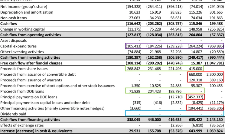
36 Table 7: cash flow statement

Table 9 shows Tesla’s cash flow statements. The company heavily relies on share issues and on the issuance of convertible debt starting in 2013 to finance its growth. In particular, it is interesting to note:

- The high capital expenses, typical of a young company ramping up its production capacity - The change in the financing structure: before 2013 it was totally financed by new equity issues

and by a subsidized debt facility by the Department of Energy; after 2013 it was financed by equity and convertible debt as well as warrants and convertible note hedges. As 2014 Tesla annual report says, “taken together, the purchase of the convertible note hedges and the sale of warrants are intended to offset any actual dilution from the conversion of the 2019 and 2021 Notes”

- Dividends are nil: since it is still a young company that needs to finance its growth, it is natural that Tesla does not pay any dividend and it is not expected to do so.

Cash flow statement

As of 31/12 in '000 2010A 2011A 2012A 2013A 2014A

Net income (group's share) (154.328) (254.411) (396.213) (74.014) (294.040)

Depreciation and amortization 10.623 16.919 28.825 115.226 301.665

Non cash items 27.063 34.230 58.631 74.634 191.863

Cash flow (116.642) (203.262) (308.757) 115.846 199.488

Change in working capital (11.175) 75.228 44.942 148.958 (256.825)

Cash flow from operating activities (127.817) (128.034) (263.815) 264.804 (57.337)

Asset disposals - - - -

-Capital expenditures (105.413) (184.226) (239.228) (264.224) (969.885)

Other investing activities (74.884) 21.968 32.298 14.807 (20.559)

Cash flow from investing activities (180.297) (162.258) (206.930) (249.417) (990.444) Free cash flow after fiancial charges (308.114) (290.292) (470.745) 15.387 (1.047.781)

Proceeds from share issues 268.842 231.468 221.496 415.000

-Proceeds from issuance of convertible debt - - - 660.000 2.300.000

Proceeds from issuance of warrants - - - 120.318 389.160

Proceeds from exercise of stock options and other stock issuances 1.350 10.525 24.885 95.307 100.455

Proceeds from DOE loans 71.828 204.423 188.796 -

-Principal payments on DOE loans - - (12.710) (452.337)

-Principal payments on capital leases and other debt (315) (416) (2.832) (8.425) (11.179) Other financing activities (mainly convertible notes hedges) (3.660) - - (194.441) (635.306)

Dividends paid - - - -

-Cash flow from financing activities 338.045 446.000 419.635 635.422 2.143.130

Effects of exchange rates - - (2.266) (6.810) (35.525)

(37)

37

In conclusion, Tesla looks like a young company that needs important sources of financing to build its manufacturing capacity and to grow. It looks like 2013 has been a turning point for Tesla. The introduction of Model S by mid 2012 made EBITDA turn positive for the first time in 2013 and profitability increased dramatically. This growth has been financed by equity, a loan facility coming from the Department of Energy and from 2013 by convertible bonds. Those types of financings are in line with the risky profile of this growing company.

3. Financings

In this section an analysis of Tesla’s financing is done to understand how the company found the resources it needed to grow. It is interesting to see how Tesla used a diverse range of equity related financing solutions. To better understand the warrant, that has been used widely during many financing phases, an example of warrant ratchet is provided before entering into the details of Tesla’s financing.

A. Theoretical review of a Warrant ratchet

The warrant ratchet is an instrument used to limit the dilution of actual investors at the next financing round. It is a mechanism used in early stages, generally by pre-public companies, in response to a subsequent round of financing that involves issuing shares at a lower price than first-stage investors. Warrants can be either (i) full ratchet or (ii) weighted average ratchet.

Quoting Investopedia (i) a full warrant ratchet is “an anti-dilution provision that, for any shares of common stock sold by a company after the issuing of an option (or convertible security), applies the lowest sale price as being the adjusted option price or conversion ratio for existing shareholders”, whereas (ii) a weighted average ratchet applies to the weighted average share price as the adjusted option price or conversion ratio for existing shareholders.

(38)

38

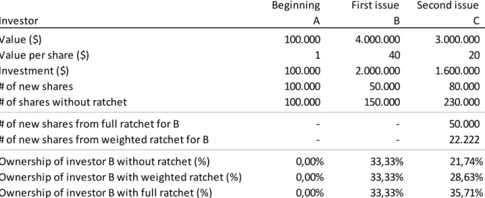
Table 10 shows an example of how a warrant ratchet can impact the final ownership of a first round investor owning a warrant.

Table 8: theoretical impact of warrant ratchets on shareholding structure

In the example it is assumed that there are three phases with three different investors entering the company’s share capital. Investor A is the founder, Investor B an early stage VC and Investor C a growth VC. It is assumed that the value of the company increases from the beginning to the first issue, but decreases from the second to the third issue resulting in a lower value per share than the first issue.

If Investor B had no warrants, it would be diluted from 33,33% to 21,74%. With a full ratchet, on the other hand, Investor B’s shareholding would increase from 33,33% to 35,71%. In fact, with a full ratchet, the minimum value per share between the first issue and the second is taken into account; since the value per share halves from the first to the second issue, the Investor B’s number of shares doubles thanks to the full ratchet. With a weighted average warrant ratchet Investor B is diluted, but by a much lower amount than without having a warrant. In fact, the number of shares Investor B is to receive are calculated using the weighted average price per share and not the minimum price, as follows:

Beginning- First issue- Second issue

-Investor A- B- C

-Value ($) 100.000 4.000.000 3.000.000

Value per share ($) 1 40 20

Investment ($) 100.000 2.000.000 1.600.000

# of new shares 100.000 50.000 80.000

# of shares without ratchet 100.000 150.000 230.000

# of new shares from full ratchet for B - - 50.000

# of new shares from weighted ratchet for B - - 22.222

Ownership of investor B without ratchet (%) 0,00% 33,33% 21,74%

Ownership of investor B with weighted ratchet (%) 0,00% 33,33% 28,63% Ownership of investor B with full ratchet (%) 0,00% 33,33% 35,71%

(39)

39

As shown by the example, it is understandable why early investors are keen to ask for some kind of protection against possible future dilutions and why warrants are so widely used in the financing phases of start-ups.

B. Tesla Equity Series A, B, C, D, E, F

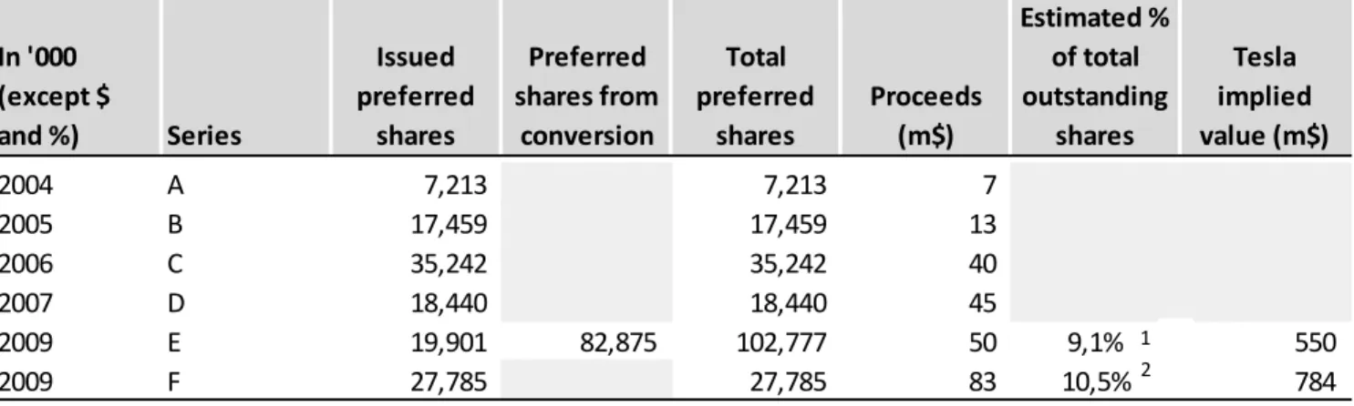
Table 9: Tesla equity financing rounds pre-IPO

Sources: Tesla annual reports and Techrunch.com Notes:

1 from Techcrunch.com 19/05/2009 2 from Techcrunch.com 15/09/2009

As it appears from Table 11, Tesla started to finance itself through convertible preferred stocks that is senior to common shares and which carries an option to convert into a fixed number of common shares, anytime after a predetermined date.

Throughout the years the company was needing an increasing amount of cash to develop its activities and raised approximately $235m of convertible preferred stock. In fact, it is common for a start-up to raise convertible preferred stock instead of common stock because it is less risky: (i) it is senior to common stock and (ii) it gives the possibility to participate in the equity potential upside by converting the preferred stock into common stock.

Very interesting are the implied valuations of the last two rounds of financings through convertible preferred stocks: in a matter of months, Tesla’s value appreciated by more than 40%.

In '000 (except $ and %) Series Issued preferred shares Preferred shares from conversion Total preferred shares Proceeds (m$) Estimated % of total outstanding shares Tesla implied value (m$) 2004 A 7,213 7,213 7 2005 B 17,459 17,459 13 2006 C 35,242 35,242 40 2007 D 18,440 18,440 45 2009 E 19,901 82,875 102,777 50 9,1% 550 2009 F 27,785 27,785 83 10,5% 784 1 2

(40)

40

C. Bridge convertible notes (converted in Series E)

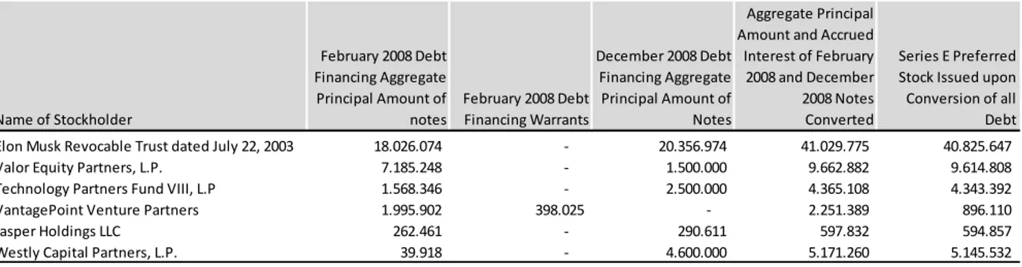
The year 2008 has been the only year during the first round of financing without a capital increase through convertible preferred stock. However, the company was needing financing, so it decided to issue senior secured convertible promissory notes in February and December 2008 for a total amount of approximately $80m in anticipation of the Series E convertible preferred stocks. Both notes had accrued interest of 10% per year.

It is interesting to note how fast Tesla converted those promissory notes in the Series E convertible preferred shares, showing (i) the need of financing by Tesla and (ii) the flexibility a start-up has in finding new streams of financings. In fact, the convertible notes had to close the financing needs gap and were all converted in convertible preferred stocks at the issuance of the Series E convertible preferred stocks at a discount of 60% to the price paid by the other investors.

Table 12 summarizes the investment in the original note by Tesla’s officers, directors and principal stockholders.

Table 10: subscription of convertible notes by major shareholders

Sources: Tesla IPO prospectus

D. Tesla’s IPO in 2010

In 2010 Tesla decided to go public to fund its growth plans. In its prospectus, Tesla states that it will use the IPO proceedings for “making aggregate capital expenditures of between $100 million and

Name of Stockholder February 2008 Debt Financing Aggregate Principal Amount of notes February 2008 Debt Financing Warrants December 2008 Debt Financing Aggregate Principal Amount of Notes Aggregate Principal Amount and Accrued Interest of February 2008 and December 2008 Notes Converted

Series E Preferred Stock Issued upon Conversion of all Debt Elon Musk Revocable Trust dated July 22, 2003 18.026.074 - 20.356.974 41.029.775 40.825.647 Valor Equity Partners, L.P. 7.185.248 - 1.500.000 9.662.882 9.614.808 Technology Partners Fund VIII, L.P 1.568.346 - 2.500.000 4.365.108 4.343.392 VantagePoint Venture Partners 1.995.902 398.025 - 2.251.389 896.110 Jasper Holdings LLC 262.461 - 290.611 597.832 594.857 Westly Capital Partners, L.P. 39.918 - 4.600.000 5.171.260 5.145.532