To cite this document:
Gouache, Thibault and Morlier, Joseph and Michon,
Guilhem and Coulange, Baptiste Operational modal analysis with non stationnary
inputs. (2013) In: IOMAC 2013, 13-15 may 2013, Guimaraes, Portugal.
O
pen
A
rchive
T
oulouse
A
rchive
O
uverte (
OATAO
)
OATAO is an open access repository that collects the work of Toulouse researchers and makes it freely available over the web where possible.
This is an author-deposited version published in: http://oatao.univ-toulouse.fr/
Eprints ID: 8631
Any correspondence concerning this service should be sent to the repository administrator: [email protected]
OPERATIONAL MODAL ANALYSIS WITH NON
STATIONNARY INPUTS
Thibault Gouache1, Joseph Morlier2, Guilhem Michon3, Baptiste Coulange4
ABSTRACT
Operational modal analysis (OMA) techniques enable the use of in-situ and uncontrolled vibrations to be used to lead modal analysis of structures. In reality operational vibrations are a combination of numerous excitations sources that are much more complex than a random white noise or a harmonic. Numerous OMA techniques exist like SSI, NExT, FDD and BSS. All these methods are based on the fundamental hypothesis that the input or force applied to the structure to be analyzed is a stationary white noise. For some applications this hypothesis is reasonable. However in numerous situations, the analyzed structure is subject to harmonic and transient forces. Numerous methods and research has enabled to develop methods that are robust to such harmonic contributions. To enable OMA during pressure oscillations in solid rocket boosters, the authors propose to consider transient and harmonic inputs no longer as parasites but as the main force applied to the structure that must be analyzed. This is the case during pressure oscillations in rocket boosters. We propose the use of phase analysis adapted to a transient context to conduct operational modal analysis under a harmonic transient input. This time-based novel OMA method will be exposed. The theoretical developments and algorithmic implementations are exposed. First tests have been conducted on laboratory single degree of freedom setup to validate this new OMA technique and are reported here.
Keywords: , Operational, Modal, Analysis, Transient, Phase, Pressure Oscillations, Solid rocket motors
1. INTRODUCTION
1.1. Classical operational modal analysis
Most Operational Modal Analysis (OMA) techniques are based on a fundamental hypothesis: the unknown and unmeasured input of the studied system or structure is stationary white Gaussian noise.
1 Dr, Cornis SAS, [email protected]
2 Dr, Université de Toulouse/ICA/ISAE, [email protected] 3 Dr, Université de Toulouse/ICA/ISAE, [email protected] 4 Dr, Cornis SAS, [email protected]
2
The Natural Excitation Techniques method, which uses auto and cross correlation is based on this hypothesis [1]. The Frequency Domain Decomposition method, based on singular value decomposition is also built on the hypothesis of spatially and harmonically white input [2]. Stochastic subspace identification methods (using covariance or subspace technique) [3] are another example of such techniques. These techniques have been applied to a various number of structures: bridges [4], aircrafts in flight [5], ship structures [6], wind turbines [7], commercial satellites and many other structures [8].
But, in addition to white noise, the input can contain some dominant frequency components (due to a running engine for example) [3]. The input of the system can also evolve in time and induce transient effects [5]. To take into account the limit imposed to OMA techniques by the fundamental stationary white noise input assumption, two general approaches are used. The first one consists in developing methods that are robust and insensible to the violations of this hypothesis. In [9], B Cauberghe et al. studied the robustness of their frequency-domain OMA technique against transient effects. The second approach used is to enrich or to relax the fundamental hypothesis of white noise. The OMA methods based on the cesptrum domain relax the classical OMA hypothesis: they only suppose that input is cepstrum short [10]. It is also possible to suppose that the structure input is a superposition of Gaussian white noise and a harmonic excitation. In [11], R. Pintelon et al. proposed three methods to suppress unknown harmonic time varying pulsations. Generally, enriching the fundamental hypothesis of OMA gives birth to new OMA techniques like those proposed by P. Mohanty and D.J. Rixen [12-15].
1.2. Transient vibrations (solid rocket motors and many other cases)
A large number of transient phenomenon exist and this should be taken into account in OMA techniques [5; 11]. Transient pressure oscillations are often observed in Solid Rocket Motors (SRM) [16]. Everyday structures are also subject to transient inputs: plane fluttering [17], wind gusts on bridges, waves on dams and, earthquakes on buildings are some examples. Instead of developing robust OMA algorithms against transient effects like in [9], it is proposed here to take into account the presence of transient harmonic excitations in a structure's input to develop a new OMA technique based on transient inputs.
1.3. Paper layout
After describing the properties of resonance, the first section of this paper proposes the novel definition of "Transient Phase" (TP). To better understand the new notion of transient phase, a Single Degree Of Freedom (SDOF) transient oscillator model is introduced. The second section is dedicated to the study of transient phase in the SDOF case: a mathematical parametric reduction proves that transient phase only depends on the ratios of four characteristic time quantities and some typical transient phase profiles are exposed. This allows the authors to propose a SDOF OMA technique based on the existence of transient regimes. Section three presents the SDOF experimental setup, the experimental validation of mathematical parametric reduction and the validation of the proposed SDOF OMA technique. Finally, to accommodate this new SDOF OMA technique to multiple degree of freedom structures, an algorithm is proposed based on mixed time-frequency decomposition. This algorithm and the notion of transient phase are then tested on Solid Rocket Motor (SRM) firing tests.
2. RESONANCE AND PHASE IN A TRANSIENT CONTEXTE
2.1. Definition of transient phase
Resonance is identified thanks to the maximum dynamic amplification or thanks to a phase difference between input and output equal to Π/2. In the case of SRM pressure oscillations, it is very difficult to measure the forces applied to the SRM's structure. It is thus impossible to measure phase difference or dynamic amplification between output and input. With SRM pressure oscillations, a second difficulty is the non-stationary nature of the forces applied to the SRM's structure. However the transient nature of the input can be used to detect resonance. Indeed, before a system is subject to resonance it will
vibrate at a given phase. But as the forced harmonic regime is progressively imposed to the mechanical system and has the established regime is progressively reached, the phase of the system will change. Though no absolute value of phase (compared to the input phase) can be defined without access to the input, a measure of the evolution of the phase output can be observed. The evolution of output phase will be directly linked to the mechanical properties of the system and its input.
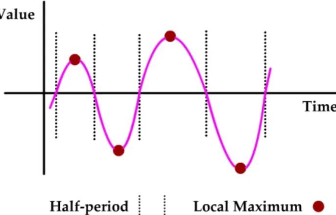
The transient response of a single degree of freedom system will have a variable amplitude. To adapt the notion of phase it is necessary to take this amplitude variation into account. The local phase of the system will thus be defined based on the local amplitude of the response. This is illustrated in Figure1.
Figure 1 Illustration of local maximum definition with variable amplitude response of mechanical system.
The transient phase phase, is thus defined by the equation here under where s(t) is the value of the response and local_max is the local maximum of the half-period as illustrated in Figure 1.
!ℎ!"#(!) = asin !(!)
!"#$!_!"# (!) (1)
Finally, since phase is always defined based on a reference, and that the input is not accessible it is necessary to define a reference. In this paper, the reference will be a pure harmonic signal whose frequency is equal to the frequency that maximizes s(t) Fourier transform.
2.2. Single degree of freedom transient model
To illustrate and test the notion of transient phase, the following transient single degree of freedom model is adopted (presented in Equation 2). x is the position; the dot is the time derivative; t is time; m,
c and k are respectively system mass, damping and stiffness; F is the harmonic amplitude; ω is the
harmonic input's frequency (in rad/s) and α(t) is a function that enables input amplitude variation.
!! + !! + !" = ! • !(!) • cos !" (2)
In this paper the function α(t) is defined by Equation 3, where α is a coefficient enabling amplitude variation speed modulation. If α is close to 0, amplitude build up is very slow, and if α is very high amplitude build up is very fast.
! ! = 0 ! ≤ 01 − !!!" ! > 0 (3) By dividing Equation 2 by m and by using linear variable changes on t and x, it is possible to show that Equation 2 depends only on the following three parameters shown in Equation 4.
! !!! ! ! ! ! !! (4)
4
Since phase is defined only by amplitude ratios, it is unchanged by linear variable changes on x and since phase is defined based on a reference it is also unchanged by linear variable changes on t. The transient phase profiles will be function only of the three parameters described in Equation 4.
2.3. Transient phase profiles
To validate the conclusions of previous section, numerical simulations of a transient single degree of freedom oscillator were conducted and the transient phase profiles were calculated based on the output of these simulations. the simulations were conducted thanks to SCILAB freeware developed by INRIA. These simulations confirmed the fact that transient phase depends only of three variables described in Equation 4.
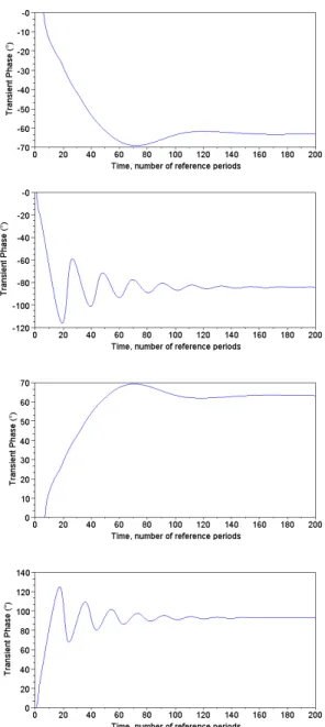
Figure 2 present examples of transient phase profiles obtained through numerical simulations. The transient phase resemble free responses. When the ratio ω/ω0 is above one the transient phase tends to decrease, when it is smaller than one the transient phase decreases. The number of oscillation depends on this ratio and the damping. Here the same damping was used for all 4 simulations. Had a smaller damping been simulated, more oscillations would have been observed.
Figure 2 Examples of transient phase profiles obtained thanks to the numerical simulations of a single degree of
freedom oscillator. The ratio ω/ω0 for each simulation is equal to 1.01, 1.05, 0.99, 0.95. For these figures
2.4. Transient phase operational modal analysis
Based on the observations in sections here above, the authors developed an Operational Modal Analysis technique based on transient phase profiles. Indeed, to identify the parameters of Equation 2 and 3, it is possible to extract from operational data the transient phase of the transient response. By using curve fit algorithms it is then possible to identify the three parameters of Equation 4 directly on the transient phase profile of the systems response. Then by using the reference frequency and the real amplitude of the response it is possible to identify ω and F/m.
The limitation of such a modal identification technique is that a correct parametric model of the input must be used. Indeed to identify the three parameters on the transient phase profile, transient profiles are simulated and feed into a curve fit algorithm to find the best fit to the experimental transient phase. However the model does not need to be highly precise. Indeed one can substitute the amplitude function α(t) defined in Equation 3 by a linear ramp or by other monotonous, continuous increasing functions without modifying significantly the transient phase profiles. The strength of this approach is very generic and that any model can be used to simulate the behavior of the system. If a mechanical system that must be identified is subject to specific inputs (time varying frequency) or has specific properties (non-linearity) it is possible to take these into account in the model.
3. EXPERIMENTAL VALIDATION
3.1. Experimental Setup
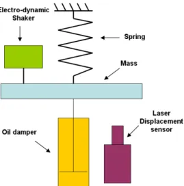
To validate the theoretical developments in sections here above and to test the single degree of freedom transient phase operational modal analysis technique proposed, a simple damped-mass-spring experimental setup was used. The experimental setup is composed of a spring attached to a mass and is described in Figure 3. The mass is guided in translation. Four different springs and three masses are used. The mass is connected to a viscous damper. The viscous damper is made of two parallel plates that bath in a cylinder full of oil.
Figure 3 Schematic of experimental setup. A spring-mass-oil damper system is activated by an electro-dynamic
shaker. Acceleration and displacement are measured.
3.2. Experimental transient phase profiles dependency on three parameters
First experiments were conducted to verify that experimental transient phase profiles are function exclusively of the three parameters in Equation 4. Figure 4 presents two transient phase profiles (one in red the other in blue), that were obtained experimentally. They were obtained with different masses, spring constants, damping, input frequency, amplitude and transient amplitude variation speed. However the six parameters were chosen in order for the ratios in Equation 4 to be all equal. The
6
experimental transient phase profiles are very close to each other (correlation of 0.98). Numerous other tests were conducted and gave similar results. This confirmed experimentally the dependency of transient phase profiles exclusively on the three parameters present in Equation 4.
Figure 4 Transient phase profiles (one in red and one in blue) versus time of two different experiments done
with m, c, k and input parameters all different but the three ratios of Equation 4 all equal.
3.3. Correlation between experimental and simulated transient phase profiles
The experimental transient phase profiles were then compared to the numerical simulated ones. A genetic curve fit algorithm was used to find the best fitting simulated phase profile. The algorithm maximizes correlation between the experimental and simulated transient phase profile. Figure 5 shows an example of an experimental transient phase profile and the best simulated fit. The agreement between numerical and experimental transient profile is very good (correlation of 0.91).
Figure 5 Transient phase profiles (experimental one in red and simulated one in blue) versus time. Correlation
between experimental and numerical transient phase is equal to 0.91.
3.4. Operational modal analysis identification results
Numerous identifications were conducted on the experimental transient data. Table 1 presents the maximum error on identification. The identification of the input and modal frequency are very precise and present highly satisfactory results. The identification of the damping can present significant errors but when compared t typical errors of other operational modal analysis methods, they are reasonable. Errors on α are much more important than errors on the other parameters. However this value is generally not identified in other operational modal analysis algorithms.
These first results are encouraging. It is possible to increase the quality of these results by proposing more efficient curve fit algorithms. These results were generated by a genetic algorithm that maximizes the correlation between the experimental transient phase and the simulated one. It is
possible to optimize other measures between the two transient phases or to implement other optimization algorithms.
Table 1 Maximum error on identification
Value Mean dispersion
ω 0.5 %
ω0 1.2 %
damping 75 %
α 180 %
4. CONCLUSIONS
Some structures like solid rocket motors used on rockets to launch satellites are subject to violent transient regimes characterized by harmonic inputs with rapidly varying amplitudes. In order to better understand these phenomenon and to better identify the modal properties of these structures, it is necessary to develop operational modal analysis techniques that can cope with transient inputs. This paper has introduced the basic building blocks and experimental and numerical explorations conducted to develop such a technique.
The notion of transient phase was introduced. Using a single degree of freedom model with a transient input, it was shown that transient phase depends only on three parameters rather than six (as does the full time response of such a system). This enables authors to propose an operational modal technique enabling the identification of a structures properties during transient inputs. The first step is the identification on the experimental transient phase of three basic parameters that define the transient phase. The other parameters are then identified by using the original time response of the system. This technique requires modeling the system's input. However the model does not need to be too precise. Experiments were conducted on mass-spring-damper setup to confirm the theoretical developments and to test the identification method. These experiments confirmed the dependency of transient phase on only three parameters. The experimental transient phase showed close agreement to the simulated ones. despite a very crude curve fit algorithm, the first modal identifications conducted with this novel method showed promising performances.
Based on this first building blocks, the modal identification of data coming from solid rocket boosters has started. The multi-degree of freedom system (that a rocket booster is) is considered as multiple independent single degree of freedom systems. Thus by filtering in the frequency domain, it is possible to use the single degree of freedom model proposed here. First results are promising and will be presented in future publications.
ACKNOWLEDGEMENTS
The authors would like to thank Prof Yves Gourniat from ISAE for allowing us to explore transient harmonic inputs. We would also like to thank Elsa Piollet and Claire Mauris-Demourioux for their help doing the experiments and their useful feed-back and ideas. finally we would like to thank Benoit Geffroy from the European Space Agency and Luc Gonidou from Centre National d'Etudes Spatiales (French space agency) for their helpful ideas and knowledge of pressure oscillations in solid motor rocket boosters.
REFERENCES
[1] G.H. James, T.G. Carne, and J.P. Lauffer (1995) The Natural Excitation Technique (NExT) for Modal Parameter Extraction from Operating Structures. Modal Analysis : The International
8
[2] R. Brincker, L. Zhang, and P. Andersen (2000) Modal Identification from Ambient Responses using Frequency Domain Decomposition. In: Proc. 18th Int. Modal Analysis Conf., San Antonio, Texas, USA.
[3] B. Peeters and G. De Roeck (2001) Stochastic Identification for Operational Modal Analysis : A Review. Journal of Dynamic Systems, Measurement, and Control, ASME, 123, pp 659-667. [4] D.J. Luscher, J. M. W. Brownjohn, H. Sohn and C. R. Farrar (2001) Modal Parameter Extraction
of Z24 Bridge Data. In: Proc. 19th Int. Modal Analysis Conf., Orlando, Florida, USA.
[5] L. Hermans and H. Van der Auwer (1999) Modal Testing and Analysis of Structures Under Operational Conditions : Industrial Applications, Mechanical Systems and signal Processing 13, 2, pp 193-216.
[6] S.-E. Rosenow, K.-D. Meinke and G. Schlottman (2005) Investigation of the Dynamic Behaviour of Ship Structures Using Classical and Operational Modal Testing. In : Proc. 1st Int. Operational
Modal Analysis Conf., Copenhagen, Denmark.
[7] N. Moller, S. Gade and H. Herlufsen (2005) Stochastic Subspace Identification Technique in Operational Modal Analysis. In : Proc. 1st Int. Operational Modal Analysis Conf., Copenhagen, Denmark.
[8] B. Peeters (2005) Industrial Relevance of Operational Modal Analysis - Civil Aerospace and Automotive Case Histories. In : Proc. 1st Int. Operational Modal Analysis Conf., Copenhagen, Denmark.
[9] B. Cauberghe, P. Guillaume, P. Verboven and E. Parloo (2003) Identification of modal parameters including unmeasured forces and transient effects. Journal of Sound and Vibration 265, pp 609-625
[10] R.B. Randall and Y. Gao (1994) Extraction Of Modal Parameters From The Response Power Cepstrum. Journal of Sound and Vibration, 176, pp 179-193.
[11] R. Pintelon, B. Peeters and P. Guillaume (2008) Continuous-time operational modal analysis in the presence of harmonic disturbances. Mechanical Systems and Signal Processing, 22, pp 1017-1035.
[12] P. Mohanty and D.J. Rixen (2004). Operational modal analysis in the presence of harmonic excitation. Journal of Sound and Vibration 270, pp 93-109.
[13] P. Mohanty and D.J. Rixen (2004) Modified SSTD method to account for harmonic excitations during operational modal analysis. Mechanism and Machine Theory 39, pp 1247-1255.
[14] P. Mohanty and D.J. Rixen (2004) A modified Ibrahim time domain algorithm for operational modal analysis including harmonic excitation. Journal of Sound and Vibration 275, pp 375-390. [15] P. Mohanty and D.J. Rixen (2006) Modified ERA method for operational modal analysis in the
presence of harmonic excitation. Mechanical Systems and Signal Processing 20, pp 114-130. [16] F. Chedevergne and G. Casalis (2006) Detailed Analysis of the Thrust Oscillations in Reduced
Scale Solid Rocket Motors. In : Proc. 42nd AIAA/ASME/SAE/ASEE Joint Propulsion Conference
and Exhibit ,AIAA, Sacremento, USA.
[17] R. Zouari. (2008) Détection Précoce de l'Instabilitée Aéroélastique des Structures Aéronautiques. PhD Thesis, Université de Rennes 1.