STATISTICAL METHODS FOR ANALYSIS AND CORRECTION OF HIGH-THROUGHPUT SCREENING DA TA
DISSERTATION PRESENTED
ASAPART~LREQUIREMENT
OF THE DOCTORA TE IN COMPUTER SCIENCE
BY
PLAMEN DRAGIEV
UNIVERSITÉ DU QUÉBEC À MONTRÉAL Service des bibliothèques
Avertissement
La diffusion de cette thèse se fait dans le rèspect des droits de son auteur, qui a signé le formulaire Autorisation de reproduire et de diffuser un travail de recherche de cycles supérieurs (SDU-522 - Rév.01-2006). Cette autorisation stipule que «conformément à l'article 11 du Règlement no 8 des études de cycles supérieurs, [l'auteur] concède
à
l'Université du Québecà
Montréal une licence non exclusive d'utilisation et de publication de la totalité ou d'une partie importante de [son] travail de recherche pour des fins pédagogiques et non commerciales. Plus précisément, [l'auteur] autorise l'Université du Québec à Montréal à reproduire, diffuser, prêter, distribuer ou vendre des copies de [son] travail de rechercheà
des fins non commerciales sur quelque support que ce soit, y compris l'lnternE;lt. Cette licence et cette autorisation n'entraînent pas une renonciation de [la] part [de l'auteur]à
[ses] droits moraux nià
[ses] droits de propriété intellectuelle. Sauf entente contraire, [l'auteur] conserve la liberté de diffuser et de commercialiser ou non ce travail dont [il] possède un exemplaire.»MÉTHODES STATISTIQUES POUR L'ANALYSE ET LA CORRECTION DES
DONNÉES DE CRIBLAGE À HAUT DÉBIT
THÈSE
PRÉSENTÉE
COMME EXIGENCE PARTIELLE
DU DOCTORAT EN INFORMA TIQUE
PAR
PLAMEN DRAGIEV
This thesis would not have been possible without the help and the support of many people. Above ali, I am heartily thankful to my two supervisors, Professor Vladimir Makarenkov from Université du Québec à Montréal and Professor Robert Nadon from McGill University for their guidance, encouragement and invaluable assistance throughout my studies that enabled me to develop understanding of the subject, to advance in and complete my research work. Special thanks, also, to my colieagues and friends at UQAM and Genome Quebec, who gave me their moral support, shared literature and assisted me with research materials. I would Iike to express my gratitude to ali professors and administrative staff at UQAM who in one way or another helped me to conclude my studies. 1 am also grateful to Fonds Québécois de la Recherche sur la Nature et les Technologies (FQRNT) for the financial support.
On a persona! leve!, 1 owe thanks to my wife, my two daughters and my parents for their love, understanding and most of ali for their patience during this multi-year adventure.
TABLE OF CONTENTS
LIST OF FIGURES ... V LIST OF TABLES ... XI LIST OF ABBREVIA TI ONS AND ACRONYMS ... XIV RÉSUMÉ ... XV ABSTRACT ... XVII CHAPTERI INTRODUCTION ... 1 1.1 High-Throughput Screening ... 1 1.2 HTS experimental errors ... 5 1.3 Hit selection ... 6
1.4 False positive and false negative hits ... 8
1.5 Sensitivity and specificity of a statistical mode! ... 8
1.6 Types of experimental error ... 9
1. 7 Within-plate HTS controls ... 10
1.8 Systematic error correction and data normalization ... 11
1.8.1 Percent of control ... 11
1.8.2 Norrna1ized percent inhibition ... 11
1.8.3 Z-score ... 12
1.8.4 Assay quality and validation ... 12
1.8.5 8-score ... 15
1.8.6 Weil correction ... 16
1.8. 7 Other HTS-related research ... 17
1. 9 Machine leaming algorithms in HTS ... 21
1.10 Decision trees ... 23
CHAPTERII
SYSTEMA TIC ERR OR DETECTION IN EXPERIMENTAL HIGH-THROUGHPUT
SCREENING ... 27 2.1 Abstract ... 29 2.1.1 Background ... 29 2 .1.2 Results ... 29 2 .1.3 Conclusions ... 29 2.2 Background ... 30
2.3 Materials And Methods ... 35
2.3.1 Data description ... 35
2.3 .2 Generating systematic error ... 36
2.3.3 Systematic error detection tests ... 38
2.4 Results And Discussion ... 42
2.4.1 Simulation 1: Detecting systematic error in individual plates ... 42
2.4.2 Simulation 2: Detecting systematic error on hit distribution surfaces ... .4 7 2.4.3 Application to the McMaster data ... 50
2.5 Conclusions ... 54
2.6 Supplementary Figures ... 57
CHAPTERIII IWO EFFECTIVE METHODS FOR CORRECTING EXPERIMENTAL HIGH-THROUGHPUT SCREENING DATA ... 76
3.1 Abstract ... 78
3.2 Introduction ... 78
3 .3 Methods ... 81
3.3.1 Data preprocessing in HIS ... 81
3.3 .2 Iwo new data correction methods ... 83
3.4 Results And Discussion ... 89
3.4.1 Simulation study ... 89
3.4.2 Analysis of the McMaster Test assay ... 98
3.5 Conclusion ... 1 08 3.6 Supplementary Materials ... 110
3.6.1 t-test applied in the HIS context ... 110
3.6.2 x2 goodness-of-fit test applied in the HIS context.. ... 111
Ill
CHAPTERIV
ST A TISTICAL METHODS FOR THE ANAL YSIS OF EXPERIMENTAL
HIGH-THROUGHPUT SCREENING DATA OOOOOOOOOOOOOOOOOOOOOOOOOOOOOOOOOOOOOOOOOOOOOOOOOOOOOOOOOOOOOOooooooOooooooooooo112 401 Abstract ooooooooooooooooooooooooooooooooooooooooooooooooooooooooooooooooooooooooooooooooooooooooooooooooooooooooooooooooooooooooooo 114 402 Introduction OOOOOOOOOOOOOOOOOOOOOOOooOOOOOOOOO OOOOOOOOOOOOOOOOOOOOOOOOOOOOOOOOOOOOOOOOOOOOOOOOOOOOOOOOOOOOOOOOOOoOOOOOOOOOOOoOooO 114 4.3 Analysis of the hit and no hit data in the Mc Mas ter Test datas et OOOOOOOOOOOOOOOOOOooOoOOOOoOoOooOoo 115 4.4 Polynomial RDA to establish relationships between hit/no hit outcomes and values of
chemical descriptors 0 00 00 0 00 0 0000 000 0 0 0 0 0000 000 000 000 0 0 000 000 000 00 00 0 00 00 0 000 0 000 0 000 0 000 000 0 Oo Ooo 0000 Ooo 0 0 0 00 0 00 0 00 0 00 0 00 0 118 405 Prediction of experimental HTS results using decision trees and neural networksooooooooo 120 406 Probability-based hit selection method oooooooooooooooOOooooooooooooooOOoooooooooooooooooooooooooooooooooooooooooo 122 40 7 New measures for assay quality estimation depending on the number of replicates 000000 131 408 Discussion and future developmentsoooooooooooooooooooooooooooooooooooooooooooooooooooooooooooooooooooooooooooooool40 CONCLUSION 0000000000000000000000000000000000 ooooooooooooooooooooooooooooooooooooooooooooooooooooooooooooooooooooooooooooooooooo 142 APPENDIXA
HTS HELPER SOFTWAREooooooooooooooooooooooooooooooooooooooooooooooooooooooooooooooooooo ... oooooooooooooooooooooooo148 Ao1 HTS Helper Utility ... o ... 148 A.2 Using HTS Helper Utility ... 0 ... 150 A.3 HTS Helper Command Line Interface ... 0 152 Syntax ... o .... ooo ... o ... o .... o .. ooooooooooooooooooo ... ooooooooooooooooooooooooooooooooooooooooooooooooooooooo .... o .. 152 Parameters ... o 0 .. 0 .. 0 0 0 .... 0 .. 0 0 .. o 0 .... o 0 000 ... o 0 0 .. o 0 0 0 0 0 0 0 0 0 0 00 0 .. 00 0 00 0. ooo 0 0 .. 0 000 0 0 0 0 00 00 0 .. 0 0 00 0 0 0 .. o .. 0 .. o 00 0 0 0 0 0 152 APPENDIXB
SOURCE CODE OF THE HTS HELPER UTILITY (VER 1.0) ooooooooooooooooooooooooooooooooooooooooo 154 ProgramoCSo .. ooooooooooooooooooo ... ooooooooooooO OOOOooOOoooooooooooooooooooooooooooooooooooooooooooooooooooooooooooooooooooooo .... 154 UserlnterfaceocS .. ooooooooooooo ... o ... o .. ooooooooooOOooOOOooOooOooooooooOooooooooooooooooooooooooo ... oooooooooOooOooOooOoo0154 CommandLineocs OooOOooooOooOOOooooOOooOOooooOOO OOOOooOooOOOooOOOOOoooooOooOoooooooooooooooooooooooooooooooooooooooooooooooooooooo 155 HTSDataocs .. 0 .. o 0 0 .. oo .... o .. o ... o ... o 0 ... o 0 ... 0 .... o 0 0 0 .. o .. 0 .... 00 0 .... 0 .. 0 0 .. 0 .. 0 000 0 .... 000 0 000 0 00 00 0 .. 0 00 0 00 0 .. 0 161 Plateocs 000000000000000000000000000000000000000000000000 0000000000000000000000000000000000000000000000000000000000000000000000000000000000 164 Dataset.cs .... 00 .. 00 00 0 0 00 .. 0 .. 0 00 00 0 .... 0 00 00 0 .. 0 0 00 0 0 .. 0 .. 0 0 ... 0 0 0 0 .. 0 0 0 0 0 ... 0 .... 0 .. 0 .. 0 0 0 0 0 ... 0 0 .. 0 0 .... 0 .. 0 .. 0 .. 0 .. 0 l 73 WellDataocs .. o .. o .... oo .... o .. oooooooo ... oooo .... o .... o ... o ... o ... o .... oo ... ooooooooooooooooooooooooo 177 GoCSoooooooooooooooooooooooooooooooooooooooooooooooooooooooooooooooooooooooooooooooooooooooooooooooooooooooooooooooooooooooooooooooooooooooo 178 HTSFileReaderocs ooooooooooooooooooooooooooooooooooooooooooooooooooooooooooooooooooooooooooooooooooooooooooooooooooooooooooooooooo 182 HTSFileWriterocs oooooooooooooooooooooooooooooooooooooooooooooooooooooooooooooooooooooooooooooooooooooooooooooooooooooooooooooooooo 193 HTSHelperocs 00000000 000000000000 .... o .. oo 0000000000000 0 00 0000 0 .... 0 .. 00 .. 000 .. 0 ... 0 ... o ... 0 0 .. o 0 .. o .. o 0 .. oo 0 .. 0 .. 0 .. o .... 198
LIST OF FIGURES
Figure Page
1.1 Drug development process (source: Malo et al. 2006) ... 2 1.2 Size of corporate screening collections over time. This figure shows that the
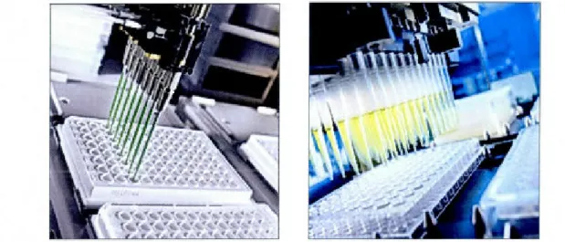
screening collections of four pharmaceutical companies from 2001 differ dramatically from those from 2009. Data taken from GlaxoSmithKline, Novartis, Sanofi-Aventis and Wyeth (now part of Pfizer) companies (source: Macarron et al. 2011) ... 3 1.3 High-throughput screening equipment (source: http://www.ingenesys.co.kr) ... 4 1.4 HTS plates with: 96 wells (8 rows x 12 columns), 384 wells (16 rows x 24 columns)
and 1536 wells (32 rows x 48 columns), (source: Mayrand Fuerst 2008) ... 5 1.5 A typical HTS plate layout (source: Malo et al. 2006) for a 96-well plate ... 10 1.6 An examp1e of a decision tree where c1 and c2 are constants such that c1>c2 .•••.•••.•••..••. 24 1.7 An example of a multilayer feed-forward network ... 25 2.1 Systematic error in experimental HTS data. Hit distribution surfaces for the
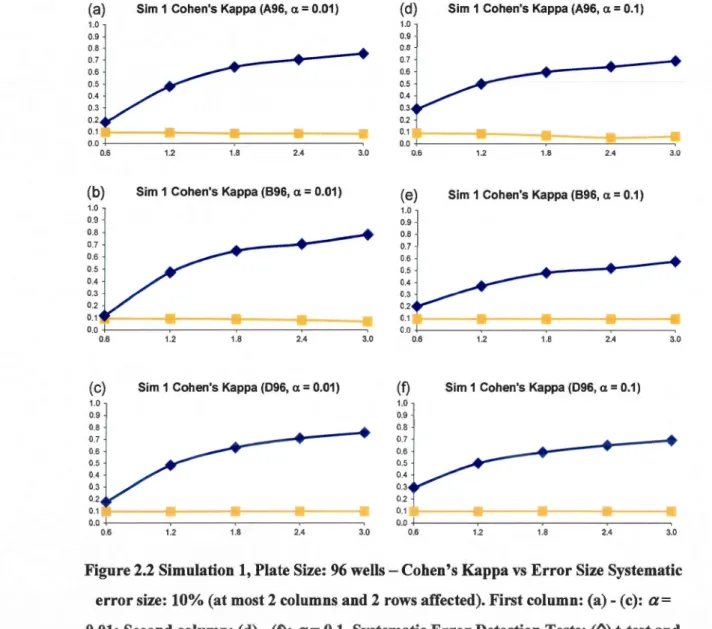
McMaster (cases (a) and (b)- 1250 plates- Elowe et al. 2005) and Princeton (cases (c) and (d) - 164 plates- (Helm et al. 2003) Universities experimental HTS assays. Values deviating from the plate means for more than 2 standard deviations - cases (a) and (c), and for more than 3 standard deviations- cases (b) and (d) were selected as hits. The weil, row and column positional effects are shown (the wells containing controls are not presented) ... 34 2.2 Simulation 1, Plate Size: 96 wells- Cohen's Kappa vs Error Size Systematic error
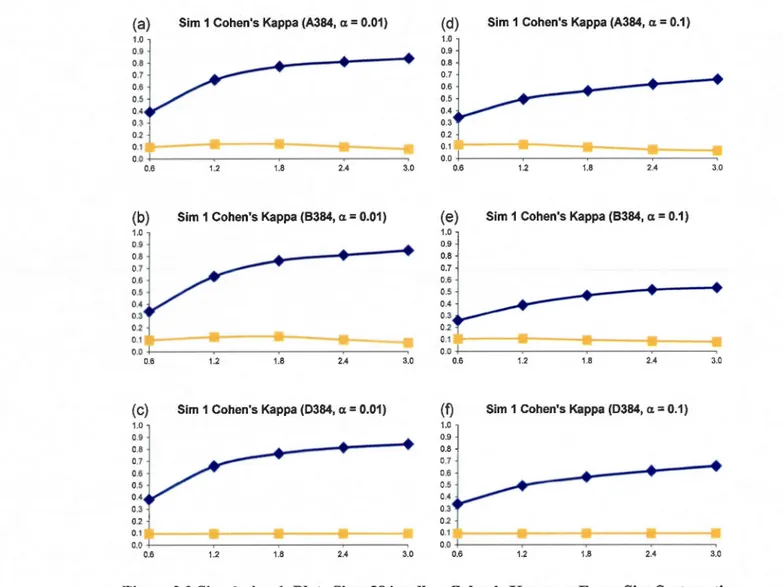
size: 10% (at most 2 columns and 2 rows affected). First column: (a)- (c): a= 0.01; Second column: (d) - (f): a= 0.1. Systematic Error Detection Tests: (0) t-test and (0) K-S test. ... 44 2.3 Simulation 1, Plate Size: 384 wells- Cohen's Kappa vs Error Size Systematic error
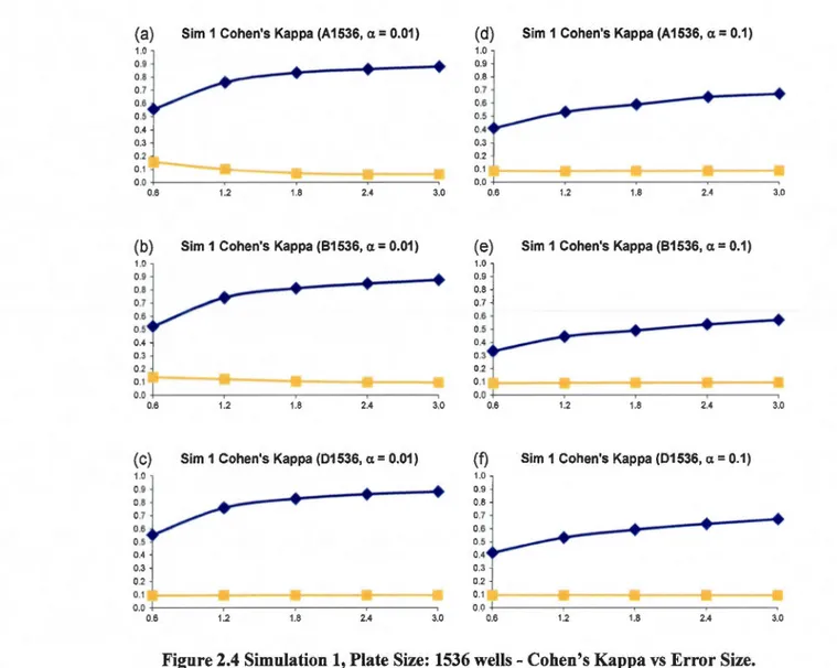
size: 10% (at most 4 columns and 4 rows affected). First column: (a)-(c): a= 0.01; Second column: (d)- (f): a= 0.1. Systematic Error Detection Tests: (0) t-test and (0) K-S test. ... 45 2.4 Simulation 1, Plate Size: 1536 wells- Cohen's Kappa vs Error Size. Systematic error
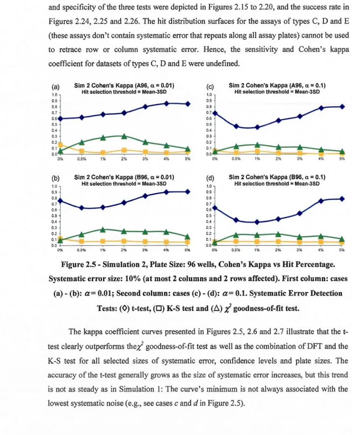
size: 10% (at most 8 columns and 8 rows affected). First column: (a)- (c): a= 0.01; Second column: (d)- (f): a= 0.1. Systematic Error Detection Tests: (0) t-test and (0) K-S test. ... 46 2.5 Simulation 2, Plate Size: 96 wells, Cohen's Kappa vs Hit Percentage. Systematic
-(b): a= 0.01; Second column: cases (c)- (d): a= 0.1. Systematic Error Detection Tests: (0) t-test, (0) K-S test and (ii);( goodness-of-fit test... ... 48 2.6 Simulation 2, Plate Size: 384 wells, Cohen's Kappa vs Hit Percentage. Systematic
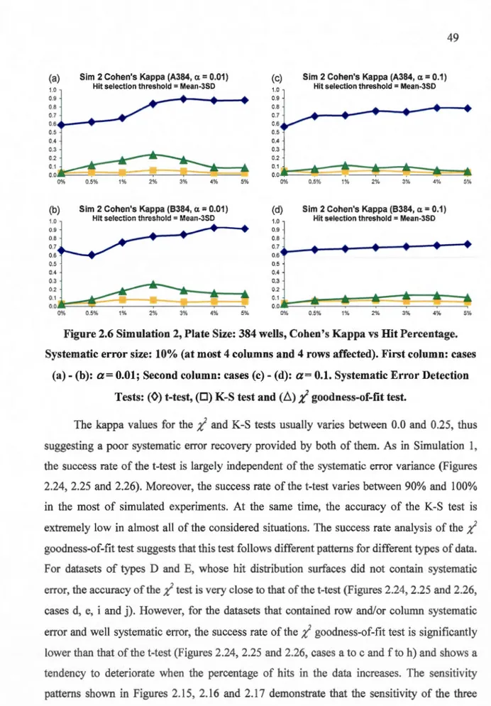
error size: 10% (at most 4 columns and 4 rows affected). First column: cases (a) -(b): a= 0.01; Second column: cases (c)- (d): a= 0.1. Systematic Error Detection Tests: (0) t-test, (0) K-S test and (ii);( goodness-of-fit test... ... 49 2.7 Simulation 2, Plate Size: 1536 wells, Cohen's Kappa vs Hit Percentage. Systematic
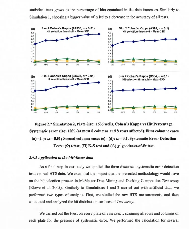
error size: 10% (at most 8 columns and 8 rows affected). First column: cases (a)-(b ): a= 0.01; Second column: cases ( c) - ( d): a= 0.1. Systematic Error Detection Tests: (0) t-test, (0) K-S test and (ii);( goodness-of-fit test... ... 50 2.8 Intersections between the original set of hits (96 hits in total) and the sets of hits
obtained after the application of the B-score ( 411 hits in total; the method was carried out only on the plates where systematic error was detected) and Weil correction methods (1 02 hits in total) computed for McMaster Test assay. The JL-2.29SD hit selection threshold was used to select hits ... 54 2.9 Simulation 1, Plate Size: 96 wells - Sensitivity (True Positive Rate). Systematic
error size: 10% (at most 2 columns and 2 rows affected). First column: cases (a)-( c ): a= 0.01; Second column: cases ( d) -(f): a= 0.1. Systematic Error Detection Tests: (0) t-test and (0) K-S test. ... 57 2.10 Simulation 1, Plate Size: 384 wells- Sensitivity (True Positive Rate). Systematic
error size: 10% (at most 4 columns and 4 rows affected). First column: cases (a)-(c): a= 0.01; Second column: cases (d)- (f): a= 0.1. Systematic Error Detection Tests: (0) t-test and (0) K-S test. ... 58 2.11 Simulation 1, Plate Size: 1536 wells - Sensitivity (True Positive Rate). Systematic
error size: 10% (at most 8 columns and 8 rows affected). First column: cases (a) -(c): a= 0.01; Second column: cases (d)- (f): a= 0.1. Systematic Error Detection Tests: (0) t-test and (0) K-S test. ... 59 2.12 Simulation 1, Plate Size: 96 wells - Specificity (True Negative Rate). Systematic
error size: 10% (at most 2 columns and 2 rows affected). First column: cases (a)-(e): a= 0.01; Second column: cases (f)- U): a= 0.1. Systematic Error Detection Tests: (0) t-test and (0) K-S test. ... 60 2.13 Simulation 1, Plate Size: 384 wells- Specificity (True Negative Rate). Systematic
error size: 10% (at most 4 colurnns and 4 rows affected). First column: cases (a)-(e): a= 0.01; Second column: cases (f)- U): a= 0.1. Systematic Error Detection Tests: (0) t-test and (0) K-S test. ... 61 2.14 Simulation 1, Plate Size: 1536 wells- Specificity (True Negative Rate). Systematic
error size: 10% (at most 8 columns and 8 rows affected). First column: cases (a)-(e): a= 0.01; Second column: cases (f)- U): a= 0.1. Systematic Error Detection Tests: (0) t-test and (0) K-S test.. ... 62
VIl
2.15 Simulation 2, Plate Size: 96 wells -Sensitivity (True Positive Rate). Systematic error size: 10% (at most 2 columns and 2 rows affected). First column: cases (a)- (b): a= 0.01; Second column: cases (c)- (d): a= 0.1. Systematic Error Detection Tests: (0) t-test, (0) K-S test and (6)
i
goodness-of-fit test. ... 63 2.16 Simulation 2, Plate Size: 384 wells - Sensitivity (True Positive Rate). Systematicerror size: 10% (at most 4 columns and 4 rows affected). First column: cases (a) -(b): a= 0.01; Second column: cases (c) - (d): a= 0.1. Systematic Error Detection Tests: (0) t-test, (0) K-S test and (6) ;(- goodness-of-fit test... ... 64 2.17 Simulation 2, Plate Size: 1536 wells - Sensitivity (True Positive Rate). Systematic
error size: 10% (at most 8 columns and 8 rows affected). First column: cases (a) -(b): a= 0.01; Second column: cases (c)- (d): a= 0.1. Systematic Error Detection Tests: (0) t-test, (0) K-S test and (6)
i
goodness-of-fit test... ... 65 2.18 Simulation 2, Plate Size: 96 wells - Specificity (True Negative Rate). Systematicerror size: 10% (at most 2 columns and 2 rows affected). First column: cases (a) -(e): a= 0.01; Second column: cases (f)- U): a= 0.1. Systematic Error Detection Tests: (0) t-test, (0) K-S test and (6)
i
goodness-of-fit test... ... 66 2.19 Simulation 2, Plate Size: 384 wells - Specificity (True Negative Rate). Systematicerror size: 10% (at most 4 columns and 4 rows affected). First column: cases (a)-(e): a= 0.01; Second column: cases (f)- U): a= 0.1. Systematic Error Detection Tests: (0) t-test, (0) K-S test and (6)
i
goodness-of-fit test... ... 67 2.20 Simulation 2, Plate Size: 1536 wells- Specificity (True Negative Rate). Systematicerror size: 10% (at most 8 columns and 8 rows affected). First column: cases (a) -(e):
a
0= 0.01; Second column: cases (f)-U):a
0= 0.1. Systematic Error Detection Tests: (0) t-test, (0) K-S test and (6)i
goodness-of-fit test... ... 68 2.21 Simulation 1, Plate Size: 96 wells - Success Rate. Systematic error size: 10% (atmost 2 columns and 2 rows affected). First column: cases (a)- (e): a= 0.01; Second column: cases (f) -U): a= 0.1. Systematic Error Detection Tests: (0) t-test and (0) K-S test. ... 69 2.22 Simulation 1, Plate Size: 384 wells- Success Rate. Systematic error size: 10% (at
most 4 columns and 4 rows affected). First column: cases (a)- (e): a= 0.01; Second column: cases (f) -U): a= 0.1. Systematic Error Detection Tests: (0) t-test and (0) K-S test. ... 70 2.23 Simulation 1, Plate Size: 1536 wells- Success Rate. Systematic error size: 10% (at
most 8 columns and 8 rows affected). First column: cases (a)- (e): a= 0.01; Second column: cases (f)- U): a= 0.1. Systematic Error Detection Tests: (0) t-test and (0) K-S test. ... 71 2.24 Simulation 2, Plate Size: 96 wells - Success Rate. Systematic error size: 10% (at
most 2 columns and 2 rows affected). First column: cases (a)- (e): a= 0.01; Second column: cases (f)-U): a= 0.1. Systematic Error Detection Tests: (0) t-test, (0) K-S test and ( 6)
i
goodness-of-fit test... ... 722.25 Simulation 2, Plate Size: 384 wells - Success Rate. Systematic error size: 10% (at most 4 columns and 4 rows affected). First column: cases (a)-(e): a= 0.01; Second column: cases (f)-U): a= 0.1. Systematic Error Detection Tests: (0) t-test, (D) K-S test and (L.)
i
goodness-of-fit test... ... 73 2.26 Simulation 2, Plate Size: 1536 wells - Success Rate. Systematic error size: 10% (atmost 8 columns and 8 rows affected). First column: cases (a)- (e): a= 0.01; Second column: cases (f)-U): a= 0.1. Systematic Error Detection Tests: (0) t-test, (D) K-S test and (L.)
i
goodness-of-fit test.. ... 74 2.27 Data distribution before and after the application of the Discrete Fourier Transform(DFT) method. Data from one of the simulated 96-well plates before and after the application of Discrete Fourier Transform. The raw data followed a normal
distribution and contained random error on/y (i.e., systematic error was not added). The raw data show agreement with the normal distribution, both graphically (case a) and by the Kolmogorov-Smirnov test (KS = 0.03, p = 0.5). However, after the application of Discrete Fourier Transform, the data deviate from normality as shown in the graph (case b) and by the Kolmogorov-Smirnov test (KS = 0.06, p = 0.0018) ... 75 3.1 Hit maps showing the presence of positional effects in the McMaster 1250-plate
assay (Elowe et al. 2005) - (a) who le assay background surface, (b) plate 1036 measurements; and in the Princeton 164-plate assay (Helm et al. 2003) - (c) whole assay background surface, ( d) plate 144 measurements. Col or intensity is proportional to the compounds' signal levels (higher signais - potential target inhibitors, are shown in red) ... 80 3.2 True positive rate and total number offalse positive and false negative hits (i.e., total
number of false conclusions) perassay for 96-well plate assays estimated under the condition that at most two columns and two rows of each plate were affected by systematic error. Panels (a) and (b) present the results obtained for datasets with the fixed systematic error standard deviation of 1.2SD. Panels (c) and (d) present the results for datasets with the fixed hit percentage rate of 1%. Methods legend: No Correction (o), B-score (~), MEA (D), t-test and MEA (0), SMP (+), t-test, and SMP (x) ... 92 3.3 True positive rate and total number of false positive and false negative hits (i.e., total
number of false conclusions) per assay for 3 84-well plate assays estimated un der the condition that at most four columns and four rows of each plate were affected by systematic error. Panels (a) and (b) present the results obtained for datasets with the fixed systematic error standard deviation of 1.2SD. Panels (c) and (d) present the results for datasets with the fixed hit percentage rate of 1%. Methods legend: No Correction (o), B-score (~), MEA (D), t-test and MEA (0), SMP (+), t-test, and SMP (x) ... 93 3.4 True positive rate and total number of false positive and false negative hits (i.e., total
number of false conclusions) perassay for 1536-well plate assays estimated under the condition that at most eight columns and two eight of each plate were affected by systematic error. Panels (a) and (b) present the results obtained for datasets with the fixed systematic error standard deviation of 1.2SD. Panels ( c) and ( d) present the
IX
results for datasets with the fixed hit percentage rate of 1%. Methods legend: No Correction (o), B-score (~), MEA (D), t-test and MEA (0), SMP (+), t-test, and SMP (x) ... 94 3.5 True positive rate and total number of false positive and false negative hits (i.e., total
number of false conclusions) perassay for 96-well plate assays estimated under the condition that systematic error affects up to 50% of rows and columns of each plate (the exact number of affected rows and columns on each plate was determinate randomly according to the uniform distribution). Panels (a) and (b) present the results obtained for datasets with the fixed systematic error standard deviation of 1.2SD. Panels ( c) and ( d) present the results for datasets with the fixed hit percentage rate of 1%. Methods legend: No Correction ( o ), B-score (~), MEA (o), t-test and MEA (0), PMP (+), t-test, and PMP (x) ... 95 3.6 True positive rate and total number of false positive and false negative hits (i.e., total
number of false conclusions) per assay for 3 84-well plate assays estimated un der the condition that systematic error affects up to 50% of rows and columns of each plate (the exact number of affected rows and columns on each plate was determinate randomly according to the uniform distribution). Panels (a) and (b) present the results obtained for datasets with the fixed systematic error standard deviation of 1.2SD. Panels ( c) and ( d) present the results for datasets with the fixed h it percentage rate of 1%. Methods legend: No Correction ( o ), B-score (~), MEA (D), t-test and MEA (0), PMP (+), t-test, and PMP (x) ... 96
3. 7 True positive rate and total number of fa! se positive and fa! se negative hits (i.e., total number of false conclusions) per assay for 1536-well plate assays estimated under the condition that systematic error affects up to 50% of rows and columns of each plate (the exact number of affected rows and columns on each plate was determinate
randomly according to the uniform distribution). Panels (a) and (b) present the results obtained for datasets with the fixed systematic error standard deviation of 1.2SD. Panels ( c) and ( d) present the results for datasets with the fixed hit percentage rate of 1%. Methods legend: No Correction ( o ), B-score
(M,
MEA (o), t-test andMEA (0), PMP (+), t-test, and PMP (x) ... 97 3.8 Hit distribution surfaces of the McMaster Test dataset for the hit selection thresholds
J-L-SD (cases a, c, e, g, i and k) and J-L-2.29SD (cases b, d, f, h, j and l) obtained for: the raw (i.e., uncorrected) data (a, b), and the data corrected by B-score (c, d), MEA (e, f), SMP (g, h), Weil Correction+ MEA (i,j), and Weil Correction+ SMP (k, 1) ... 107 4.1 The relationship between the HTS measurement values (varying from 0 to 200) and
the molecular weight (varying from 200 to 600) depicted at 6 different levels of the
ClogP descriptor. There is virtually no difference in the six presented patterns. That suggests that ClogP does not have any influence over the way molecular weight is related to the HTS measurements ... 117 4.2 Polynomial RDA correlation biplot for the McMaster Test dataset. Triangles
represent the three types of samples (D-R Hits - the consensus hits showing good
dose-response behavior; No D-R Hils- the consensus hits not showing good dose-response behavior; No-Hits- samples that are not hits). Dashed arrows represent two
binary response variables Hit/No-Hit and D-R. Solid arrows represent the chemical descriptors (10 descriptors from Table 4.1 plus 2 extra descriptors Hdon2 and Hdon x Hacc that show the biggest correlations with Hit/No-Hit and D-R variables, respectively). The lengths of the chemical descriptor arrows were multiplied by 1 0;
this does not change the interpretation ofthe diagram ... 119 4.3 ROC curves for four different group sizes used for training and test: 48 hits
+
100(case a), 500 (case b ), 1000 (case c) and 2000 (case d) no hits. The abscissa axis
represents (1-Speci.ficity), and the ordinate axis represents Sensitivity. The results of
the decision tree method are depicted by squares and those of the neural network method by triangles ... 121 A.1 HTS Helper, Windows Forms executable (version 1.0, March 22nd, 2012) ... 148
LIST OF TABLES
Table Page
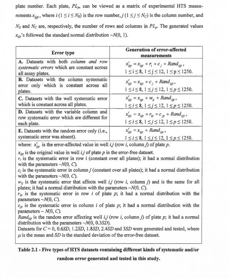
1.1 Categorization of an HTS assay quality depending on the value of Zjactor ....... 13 2.1 Pive types of HTS datasets containing different kinds of systematic and/or random
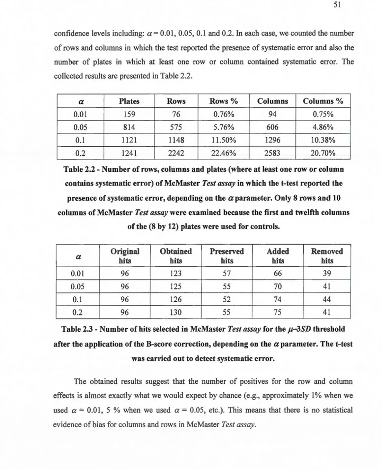
error generated and tested in this study ... 37 2.2 Number of rows, columns and plates (where at !east one row or column contains
systematic error) of McMaster Test assay in which the t-test reported the presence of
systematic error, depending on the a parameter. Only 8 rows and 10 columns of
McMaster Test assay were examined because the ftrst and twelfth columns of the (8
by 12) plates were used for control s ... 51 2.3 Number of hits selected in McMaster Test assay for the j.1-3SD threshold after the
application of the B-score correction, depending on the
a
parameter. The t-test was carried out to detect systematic err or. ... 51 2.4 Number of hits selected in McMaster Test assay for the f.1-2.29SD threshold (i.e.,threshold used by the McMaster competition organizers to select the 96 original
average hits) after the application of the B-score correction, depending on the a
parameter. The t-test was carried out to detect systematic error. ... 52
2.5 Number of hits selected in McMaster Test assay for the f.1-3SD and f.1-2.29SD thresholds after the application of the Weil Correction method ... 53
3.1 Number of hits selected by the six data correction methods for the McMaster Test dataset. The hit selection threshold of f.1-2.29SD was used ... 99 3.2 Hit distribution of the raw McMaster dataset computed for the jl-SD threshold
(mean value of hits per weil is 37.69 and standard deviation is 24.27). The ;(
goodness-of-ftt test provided the following results (;(value= 1234.23, critical value
111.14 for a= 0.01; H0 is rejected and data correction is recommended) ... 100 3.3 Hit distribution of the raw McMaster dataset computed for the j.i-2.29SD threshold
(mean value of hits per weil is 1.20 and standard deviation is 1.19). The;( goodness
-of-ftt test provided the following results (;( value = 94.0, critical value 111.14 for a = 0.01; Ho is not rejected and data correction is optional) ... 100
3.4 Hit distribution of the McMaster datas et after applying B-score normalization and
computed for the jl-SD threshold (mean value of hits per weil is 39.48 and standard
deviation is 14.67). The;( goodness-of-ftt test provided the following results (;(
value= 430.96, critical value 111.14 for a= 0.01; H0 is rejected and data correction
is recommended) ... 101
3.5 Hit distribution of the McMaster dataset after applying B-score normalization and
standard deviation is 1.89). The;( goodness-of-fit test provided the following results
(;( value= 121.10, critical value 111.14 for a= 0.01; Ho is rejected and data correction is recommended) ... 10 1 3.6 Hit distribution of the McMaster dataset after applying Matrix Error Amendment
(MEA) method and computed for the
;r-SD threshold
(mean value of hits per weil is38.48 and standard deviation is 23.96). The ;( goodness-of-fit test provided the following results (;(value= 1178.53, critical value 111.14 for a= 0.01; Ho is rejected and data correction is recommended) ... 1 02 3. 7 Hit distribution of the McMaster dataset after applying Matrix Error Amendment
(MEA) method and computed for the ;..r2.29SD threshold (mean value of hits per weil is 1.25 and standard deviation is 1.24). The;( goodness-of-fit test provided the following results (;( value = 96.80, critical value 111.14 for a = 0.01; Ho is not rejected and data correction is optional) ... 102
3.8 Hit distribution of the McMaster dataset after applying Partial Mean Polish (PMP) method and computed for the
;r-SD
threshold (mean value of hits per weil is 39.90 and standard deviation is 22.41). The;( goodness-of-fit test provided the following results (;( value = 994.27, critical value 111.14 for a= 0.01; Ho is rejected and data correction is recommended) ... 1 03 3.9 Hit distribution of the McMaster dataset after applying Partial Mean Polish (PMP)method and computed for the ;..r2.29SD threshold (mean value of hits per weil is
1.44 and standard deviation is 1.32). The ;( goodness-of-fit test provided the foilowing results (;( value = 95.78, critical value 111.14 for a= 0.01; Ho is not rejected and data correction is optional) ... 1 03 3.10 Hit distribution of the McMaster dataset after applying Weil Correction followed by
Matrix Error Amendment (MEA) method and computed for the
;r-SD
threshold (mean value of hits per weil is 35.48 and standard deviation is 9.55). The ;(goodness-of-fit test provided the following results (;( value = 203.18, critical value 111.14 for a= 0.01; Ho is rejected and data correction is recommended) ... 104 3.11 Hit distribution of the McMaster dataset after applying Weil Correction followed by
Matrix Error Amendment (MEA) method and computed for the ;..r2.29SD threshold (mean value of hits per weil is 1.36 and standard deviation is 1.37). The;( goodness-of-fit test provided the following results (;( value = 108.98, critical value 111.14 for
a= 0.01; Ho is not rejected and data correction is optional) ... 104 3.12 Hit distribution of the McMaster dataset after applying Weil Correction followed by
Partial Mean Polish (PMP) method and computed for the
;r-SD
threshold (meanvalue ofhits per weil is 35.64 and standard deviation is 9.47). The;( goodness-of-fit
test provided the foilowing results
(j
value = 198.68, critical value 111.14 for a=0.01; Ho is rejected and data correction is recommended) ... 105 3.13 Hit distribution of the McMaster dataset after applying Weil Correction followed by
Partial Mean Polish (PMP) method and computed for the ;..r2.29SD threshold (mean
XIII
test provided the following results
(j
value = 108.98, critical value 111.14 for a=0.01; Ho is not rejected and data correction is optional) ... 105
4.1 Average values of the measurements and 10 chemical descriptors for four types of
samples (consensus hits- 42 samples, average bits- 96 samples, hits having
well-behaved dose-response curves- 26 samples and the whole dataset- 50,000 samples)
from the McMaster University Test dataset. In bold, the values of chemical
descriptors showing important variation ... 116 4.2 Results obtained after applying the new probability-based hit selection method on
the raw McMaster Test dataset. Results are shown for different values of the
probability-based hit selection thresholds, Phil• varying from 0.05 to 0.95. For each
thresho1d value, the list of selected hits was compared to the official McMaster
average hit list. ... 126 4.3 Results obtained after applying the new probability-based hit selection method on
the McMaster Test dataset corrected by the Matrix Error Amendment method.
Results are shown for different values of the probability-based hit selection
thresholds, Phil, varying from 0.05 to 0.95. For each threshold value, the list of
selected hits was compared to the official McMaster average hit list. ... 127 4.4 Results obtained after applying the new probability-based hit selection method on
the McMaster Test dataset corrected by the Partial Mean Polish method. Results are
shown for different values of the probability-based hit selection thresholds, Phu,
varying from 0.05 to 0.95. For each threshold value, the list of selected hits was
compared to the official McMaster average hit list. ... 128
4.5 Results obtained after applying the new probability-based hit selection method on
the McMaster Test dataset corrected by the Well Correction followed by Matrix
Error Amendment methods. Results are shawn for different values of the
probability-based hit selection thresholds, Phil, varying from 0.05 to 0.95. For each
threshold value, the list of selected hits was compared to the official McMaster
average hit list. ... 129
4.6 Results obtained after applying the new probability-based hit selection method on
the McMaster Test dataset corrected by the Weil Correction and Partial Mean Polish
methods. Results are shown for different values of the probability-based hit selection
thresholds, Phil, varying from 0.05 to 0.95. For each threshold value, the list of
selected hits was compared to the official McMaster average hit list. ... 130
4.7 The 96 average hits from the McMaster Test assay with their MAC IDs, the first
(Ml) and the second (M2) measurement values, hit probability computed from
theoretical distribution, and false positive (FPch) and false negative (FNcr) change
rates also computed from theoretical distributions. The consensus hit are italicized .... 139
ANN Artificial neural networks DFT Discrete Fourier Transforrn FN False negative
FP False positive
HTS High-throughput screening kNN k-nearest neighbors MAD Median absolute deviation MEA Matrix Error Arnendment
PMP
Partial Mean Polish RDA Redundancy AnalysisSAR Structure-activity relationship Se Sensitivity
Sp Specificity
SVM Support vector machines TN True negative
xv
RÉSUMÉ
Durant le criblage à haut débit (High-throughput screening, HTS), la première étape dans la découverte de médicaments, le niveau d'activité de milliers de composés chimiques est mesuré afin d'identifier parmi eux les candidats potentiels pour devenir futurs médicaments (i.e., hits). Un grand nombre de facteurs environnementaux et procéduraux peut affecter négativement le processus de criblage en introduisant des erreurs systématiques dans les mesures obtenues. Les erreurs systématiques ont le potentiel de modifier de manière significative les résultats de la sélection des hits, produisant ainsi un grand nombre de faux positifs et de faux négatifs. Des méthodes de correction des données HTS ont été développées afin de modifier les données reçues du criblage et compenser pour l'effet négatifs que les erreurs systématiques ont sur ces données (Heyse 2002, Brideau et al. 2003, Heuer et al. 2005, Kevorkov and Makarenkov 2005, Makarenkov et al. 2006, Malo et al. 2006, Makarenkov et al. 2007).
Dans cette thèse, nous évaluons d'abord l'applicabilité de plusieurs méthodes statistiques servant à détecter la présence d'erreurs systématiques dans les données HTS expérimentales, incluant lei goodness-of-fit test, le t-test et le test de Kolmogorov-Smirnov précédé par la méthode de Transformation de Fourier. Nous montrons premièrement que la détection d'erreurs systématiques dans les données HTS brutes est réalisable, de même qu'il est également possible de déterminer l'emplacement exact (lignes, colonnes et plateau) des erreurs systématiques de l'essai. Nous recommandons d'utiliser une version spécialisée dut-test pour détecter l'erreur systématique avant la sélection de hits afin de déterminer si une correction d'erreur est nécessaire ou non.
Typiquement, les erreurs systématiques affectent seulement quelques lignes ou colonnes, sur certains, mais pas sur tous les plateaux de l'essai. Toutes les méthodes de correction d'erreur existantes ont été conçues pour modifier toutes les données du plateau sur lequel elles sont appliquées et, dans certains cas, même toutes les données de l'essai. Ainsi, lorsqu'elles sont appliquées, les méthodes existantes modifient non seulement les mesures expérimentales biaisées par l'erreur systématique, mais aussi de nombreuses données correctes. Dans ce contexte, nous proposons deux nouvelles méthodes de correction d'erreur systématique performantes qui sont conçues pour modifier seulement des lignes et des colonnes sélectionnées d'un plateau donné, i.e., celles où la présence d'une erreur systématique a été confirmée. Après la correction, les mesures corrigées restent comparables avec les valeurs non modifiées du plateau donné et celles de tout l'essai. Les deux nouvelles méthodes s'appuient sur les résultats d'un test de détection d'erreur pour déterminer quelles lignes et colonnes de chaque plateau de l'essai doivent être corrigées. Une procédure générale pour la correction des données de criblage à haut débit a aussi été suggérée.
Les méthodes actuelles de sélection des hits en criblage à haut débit ne permettent généralement pas d'évaluer la fiabilité des résultats obtenus. Dans cette thèse, nous décrivons une méthodologie permettant d'estimer la probabilité de chaque composé chimique d'être un
hit dans le cas où l'essai contient plus qu'un seul réplicat. En utilisant la nouvelle
méthodologie, nous définissons une nouvelle procédure de sélection de hits basée sur la probabilité qui permet d'estimer un niveau de confiance caractérisant chaque hit. En plus, de
nouvelles mesures servant à estimer des taux de changement de faux positifs et de faux négatifs, en fonction du nombre de réplications de l'essai, ont été proposées.
En outre, nous étudions la possibilité de définir des modèles statistiques précis pour la prédiction informatique des mesures HTS. Remarquons que le processus de criblage expérimental est très coûteux. Un criblage virtuel, in silico, pourrait mener à une baisse importante de coûts. Nous nous sommes concentrés sur la recherche de relations entre les mesures HTS expérimentales et un groupe de descripteurs chimiques caractérisant les composés chimiques considérés. Nous avons effectué l'analyse de redondance polynomiale (Polynomial Redundancy Analysis) pour prouver l'existence de ces relations. En même temps, nous avons appliqué deux méthodes d'apprentissage machine, réseaux de neurones et arbres de décision, pour tester leur capacité de prédiction des résultats de criblage expérimentaux.
Mots-clés : criblage à haut débit (HTS), modélisation statistique, modélisation predictive, erreur systématique, méthodes de correction d'erreur, méthodes d'apprentissage automatique
ABSTRACT
During the high-throughput screening (HTS), an early step in the drug discovery process, the activity levels of thousands of chemical compounds are measured in order to identify the potential drug candidates, called hits. A number of environmental and procedural
factors can affect negatively the HTS process, introducing systematic error in the obtained experimental measurements. Systematic error has the potential to alter significantly the outcome of the hit selection procedure, thus generating eventual false positives and false negatives. A number of systematic error correction methods have been developed for compensating for the effect of this error in experimental HTS (Heyse 2002, Brideau et al. 2003, Kevorkov and Makarenkov 2005, Heuer et al. 2005, Makarenkov et al. 2006, Malo et al. 2006, Makarenkov et al. 2007).
In this thesis, we first evaluate the applicability of severa! statistical procedures for assessing the presence of systematic error in experimental HTS data, including the ;( goodness-of-fit test, Student's t-test and Kolmogorov-Smirnov test preceded by the Discrete Fourier Transform method. We show that the detection of systematic error in raw HTS datais achievable, and that it is also possible to determine the most probable assay locations (rows,
columns and plates) affected by systematic error. We conclude that the t-test should be preferably used prior to the hit selection in order to determine whether an error correction is required or not.
Typically, systematic error affects only a few rows and/or columns of the given plate (Brideau et al. 2003, Makarenkov et al. 2007). Ali the existing error correction methods have been designed to modify ali the data on the plate on which they are applied, and in sorne cases, even ail the data in the assay. Thus the existing methods modify not only the error-biased measurements, but also the error-free measurements. We propose two new error correction methods that are designed to modify (i.e., correct) only the measurements of the selected rows and columns where the presence of systematic error has been confirmed. After the correction, the modified measurements remain comparable with the unmodified ones within the given plate and across the entire assay. The two new methods rely on the results from an error detection test to determine which plates, rows and columns should be corrected.
Our simulations showed that the two proposed methods generally outperform the popular B-score procedure (Brideau et al. 2003). We also describe a general correction procedure allowing one to correct both plate-specifie and screen-specific systematic error.
The hit selection methods used in the modem HTS do not allow for assessing the reliability of the selected hits. In this thesis, we describe a methodology for estimating the probability of each compound to be a hit when the assay contains more than one replicate.
Using the new methodology, we defme a new probability-based hit selection procedure that allows one to estimate the probability of each considered compound to be a hit based on the
available replicate measurements. Furthermore, new measures for computing the false positive and false negative change rates depending on the number of experimental assay
replicates (i.e., how these two rates would change if an additional screen replicate will be
performed), are introduced.
Further, we investigate the possibility of developing accurate statistical models for computer prediction of HTS measurements. Note that the experimental HTS process is very
expensive. The use of virtual, in silico, HTS instead of experimental HTS could lead to an important cost decline. We first focus on finding relationships between experimental HTS measurements and a group of descriptors characterizing the given chemical compounds. We carried out Polynomial Redundancy Analysis (Polynomial RDA) to prove the existence of such relationships. Second, we evaluate the applicability of two machine learning methods, neural networks and decision trees, for predicting the hit/non-hit outcomes for selected compounds, based on the values oftheir chemical descriptors.
Keywords: high-throughput screening (HTS), statistical modeling, predictive modeling, systematic error, error correction methods, machine learning methods
CHAPTERI
INTRODUCTION
1.1 High-Throughput Screening
High-throughput screening (HTS) is a large-scale highly automated process used widely within the pharmaceutical industry (Broach and Thomer 1996, Carnero 2006, Malo et al. 2006, Janzen and Bernasconi 2009). lt is employed in the early stages of the drug discovery process during which a huge number of chemical compounds are screened and the compounds activity against a specifie target measured. The goal of HTS is to identify among ali tested compounds those showing promising "drug-like" properties. As specified in Sirois et al. (2005) and Malo et al. (2006), the drug discovery could be described as a multi-step process (Figure 1.1 ):
1. Hit identification: target selection (i.e., researchers typically focus on enzymes or proteins that are essential to the survival of an infectious agent), assay preparation, primary screening;
2. Hit verification: re-testing, secondary screening and dose response curve generation;
3. Lead identification: structure-activity relationships (SAR) analysis,
establishing and confmning the mechanism of action;
4. Clinical studies: drug effectiveness evaluation, drug-to-drug interactions, safety assessment studies;
2
High-throughput screening is the backbone of the first step of the drug discovery process. At that stage, thousands of chemical compounds are tested in an initial primary screen. The identified compounds are marked for follow-up in the second step of the process when HTS is employed again for performing secondary screens of a group of pre-selected (i.e., hit) compounds (e.g., 1% of the most active compounds from the primary screen, Nelson and Yingling 2004). Typically, at !east duplicate compound measurements are recommended (Malo et al. 2006).
A biological assay
(specifie target
& reagents)
'Hils'
Secondary screen & oounter screen
'Contirmed llits~
Structure-ac!ivity relationsllip (SAR)
& medicinal chemistry
'Leads'
'Drug'
A large
libraf)'of
cllemfcal oompounds.
3
HTS is a relatively new technology that continues to advance at fast pace. The recent progress in computer technologies and robotic automation reduced significantly the cost of operating high-throughput screening facility and made the technology feasible for many small and moderate-sized organizations. The priee of experimental screening per unit also
dropped significantly bringing a considerable increase in the number of tested compounds.
Figure 1.2 (Macarron et al. 2011) shows that the use of HTS in the four selected
pharmaceutical companies more th en doubled for three of them and increased by 10 times for the fourth company during the period from 2001 to 2009.
2,0
00
,
00
0
2001
rJ) '"02005
c
~1,500,000
002
0
09
o.
E
0 u1,0
0
0,0
0
0
-
0 1.... Q) _oE
~5
0
0,
00
0
z
E
F
G
H
Company
Figure 1.2 Size of corporate screening collections over time. This figure shows that the
screening collections of four pharmaceutical companies in 2001 differ dramatically from those in 2009. Data taken from GlaxoSmithKline [E], Novartis [F], Sanofi-Aventis
[G] and Wyeth [H] (now part ofPfizer) companies (source: Macarron et al. 2011)
The steadily decreasing priees, as weil as a number of govemmental programs and initiatives (Austin 2008) allowed HTS to penetrate rapidly into the academie settings (Stein 2003, Verkman 2004, Kaiser 2008, Silber 2010). In May 2012, the website of the US Society for Laboratory Automation and Screening listed 93 academie institutions that have
established HTS facilities (SLAS 2012), while the Molecular Libraries Initiative has generated a collection of more than 360,000 compounds in a screening library for academie investigators (MLP 2012).
The modem drug discovery is no more exclusively based on chemistry. lt is a product of interdisciplinary cooperation of engineers, chemists, biologists and statisticians. Massive libraries of millions of compounds have been created using combinatorial chemical synthesis and are used as a drug-candidate base. The contemporary HTS technology is an almost fully automated process. Robots are used in ali steps of the process. They retrieve compounds from the libraries, combine them with the selected biological target, convey the compound solutions through the HTS readers and record the measured activity levels. The recent dramatic improvements in miniaturization, low-volume liquid-handling and multimodal readers increased drastically the throughput of the screening process. Figure 1.3 depicts two typical high-throughput screening systems.
Figure 1.3 High-throughput screening equipment (source: http://www.ingenesys.co.kr)
The contemporary HTS systems are capable of screening more than 100,000 compounds per day (Mayr and Fuerst 2008). At the same time, the screening-collection sizes constantly increase and are expected to grow, given the fact that the size of the "drug like" chemical space is estimated to be greater than Ix1030 compounds (Fink and Reymond 2007). High-throughput screening involves many steps, such as target selection and characterization, assay development, reagent preparation and compound screening. Each of those steps adds
5
cost proportional to the number of the compounds in the assay. Thus, despite the technological advances, HTS remains an expensive technology.
High-throughput screening assays are organized as a sequence of plates. HTS plate is a
small container, usually disposable and made of plastic. It includes a grid of small, open
concavities called wells. During the assay preparation, every compound of interest is placed in a separate well. • • • • • • • • • • •••• lt 1 ···.···~
·
···••*••••&
.
...
..
.
..
':::::::::::::
1mt
···~ aaaaaaaaaaaaakK~ •••••••••••••m~~ ···~ ••••••••••••••utlt: ···&~ · •••••••••••••~ee ••••••••••••••m~•••••••••••••••
c
• • • • • • • • • • • • •• 11:111 ···•••~r • • • • • • • • • • • • ••• !1!' ••• • • • • • • • • •• • 111! • •• • • • • • • • • •• • 11111 ···~~:~ ~···~8 1:
:
:
:
::::
::::::lri
;
Figure 1.4 HTS plates with: 96 wells (8 rows x 12 columns), 384 wells (16 rows x 24 columns) and 1536 wells (32 rows x 48 columns), (source: Mayrand Fuerst 2008)
A typical HTS plate consists of 96 wells arranged in 8 rows and 12 columns. Along
with the tendency ofminiaturization in HTS, plates with 384 and 1536 were also created (see
Figure 1.5). The plates with more wells usually have the same dimensions but contain smaller
wells. During the screening process, ali the wells on the plate are examined and the activity
leve) of their content is registered as a single numeric value. Th us, the results of screening one plate can be represented as a matrix of numeric values where the measurements are
arranged in the same layout as the compounds on the plate.
1.2 HTS experimental errors
Since the appearance of the first HTS systems, 15-20 years ago, a lot of efforts have
been made to improve the speed, the capacity and the precision of HTS equipment (Macarron
2006, Pereira and Williams 2007, Houston et al. 2008). The contemporary HTS systems are
differences in the compounds' activity levels. That remarkable sensitivity, otherwise an asset,
makes the HTS process prone to errors. Many environmental factors, including variations in the electricity, temperature, air flow and light intensity, may affect HTS readers (Makarenkov et al. 2007). Equipment malfunctions, such as robotic failures, poor pipette delivery, glass
fogging or needle clogging, may also cause erroneous readings. Assay miniaturization and especially work with very small liquid volumes cao cause fast and significant concentration changes due to reagent evaporation. Therefore, procedural factors such as differences in the time compounds await to be processed create inequalities among the experimental measurements. In the context of HTS, an experimental error (or simply an error) denotes the case when the measurement obtained during the screening does not reflect the real compound activity either because of a failure during the reading procedure or because the conditions at which the activity was measured differed from the planned ones. Systematic error affects the HTS data by either over- or underestimating the measurements of sorne of the compounds. With the appearance of the second generation HTS systems in 2001 (Mayr and Fuerst 2008),
a strong focus was put on the quality of the selected hits, i.e., to ensure lower readout artifacts. HTS laboratories have pioneered and implemented rigorous quality assurance methods (Macarron et al. 2011), such as liquid handler and reader performance monitoring (Taylor et al. 2002), Z trend monitoring (Zhang et al. 1999) and regular usage of pharmacological standards (Coma et al. 2009). Despite the remarkable quality improvements,
the experimental error remains a major hindrance in high-throughput screening, and handling
this error becomes even of a greater importance as our dependence on the technology increases.
1.3 Hit selection
Hit selection is the last step of the high-throughput screening process. At this step, the compounds with the best activity values are selected for further investigation. The
compounds selected in such a way are called hits (Malo et al. 2006). The hit selection is based on comparability of the activity measurements. Depending on the type of the screened assay the researches may be interested either in the compounds showing the highest activation properties (activation assays - the goal here is to activate the given target) or the highest inhibition properties (inhibition assays -the goal here is to inhibit the given target).
7
There exist four different strategies for selecting hits (Malo et al. 2006):
1. Hits are selected as a fixed percentage of ali compounds, those having the highest activity levels (for example: top 1 %). This strategy, and especially the number of selected hits, is dictated by resource availability and other project constraints. This method is not usually recommended because a fixed, in advance, number of compounds does not usually reflects the number of really active compounds in the assay;
2. Hits are identified as compounds whose activity measurements exceed sorne fixed threshold. The hit-cutting threshold can be specified as an absolute value or as a percentage of the maximum possible activity leve!. In arder to achieve quality results using such a threshold, the advanced knowledge about the expected activity levels is required;
3. Simi1ar to the second strategy, hits are selected to exceed a hit-cutting threshold,
but the threshold is calculated to reflect the specifies of the actual data. This threshold is usually expressed in terms of the mean value f.1 (the median can be also used) and the standard deviation CJ of the measurements, with the most widely used threshold of .u--3Œ(inhibition assays) and f..1+3Œ(activation assays). This strategy can be applied globally for the whole assay when the mean and standard deviation are calculated using ali measurements of the assay, or altematively, on the plate-by-plate basis when the mean and the standard deviation are calculated separately for each plate using only the associated plate's
measurements.
4. Statistical testing with replicates was recommended by Malo et al. 2006) for a better hit identification. More specifically, to get around the small sample size problem that is known to produce serious problems with the t-test, Malo et al. 2006) recommended using "shrinkage tests" (see also Allison et al. 2006). They provided a specifie example of one particular shrinkage test - the Random
1.4 False positive and false negative bits
The presence of error in experimental HTS data may affect the accuracy of the hit selection campaign. Working with the measurements that do not correctly represent the real compound activity levels may cause the situation where sorne compounds are mistakenly selected as hits: this situation is known as Type 1 error and the selected compounds are called false positives (FP). It is also possible that sorne active compounds are overlooked, i.e., they have not been selected as hits: this situation is known as Type II error and the affected compounds are called jalse negatives (FN). Ali the active compounds that are correctly identified as hits are defined as true positives (TP) and the correctly identified inactive compounds are defined as true negatives (TN).
1.5 Sensitivity and specificity of a statistical model
With its ability to separate the compounds into two groups, bits and non-hits, the
high-throughput screening process constitutes a binary classifier. Sensitivity (Se) and Specificity (Sp) are two statistical measures used to evaluate the performance of such classifiers. The sensitivity ofthe model can be defined as follows:
TP
Se=-
-TP+FN
In the context of HTS, Sensitivity represents the proportion of the active compounds that were selected as hits. The sensitivity value of 1 (or 100% if expressed as a percentage) indicates that all active compounds were successfully identified as hits, whereas the value of 0 means that ali active compounds were overlooked as false negatives.
The value of Specificity can be calculated using the following formula:
S _ TN
9
In the context of HTS, Specificity represents the proportion of the non-hit compounds that were not selected as hits. Specificity value of 1 (or 100% if expressed as a percentage) indicates that no inactive compounds were incorrectly identified as hits.
1.6 Types of experimental error
Momentary variations in the HTS experimental conditions introduce random errors in the screening data that affect single or limited number of compounds only. Random error unpredictably lowers or raises the values of sorne of the screened measurements. Random errors can affect as weil the hit selection process (Kevorkov and Makarenkov 2005). If a further increase of the HTS precision is required, in regards to random error, then replicated measurements should be used, i.e., multiple instances of the compounds should be screened (Lee et al. 2000, Nadon and Shoemaker 2002). It is also important to note that this type of error is usually very difficult to detect in HTS using standard quality control and performance monitoring techniques.
Another type of error, systematic error, can as weil be present in HTS data. Systematic error biases experimental HTS results by systematically over- or underestimating the compounds true activity levels and affects multiple compounds of the given plate or given assay. Systematic error is usually location dependent (Brideau et al. 2003). lt generates repeatable local artifacts that may affect only a single plate, a group of severa] plates or even ali plates of the assay. Within the plates, the compounds affected by systematic error are usually located in the same row or column, very often at the edges of the given plate -situation known as edge effect (Cheneau et al. 2003, Iredale et al. 2005, Carralot et al. 2012). It is also possible that systematic error affects only the compounds located at the specifie weil locations on ali the plates or majority of plates across the assay (Makarenkov et al. 2007).
Systematic error has the potential to affect significantly the hit selection process, thus resulting in the generation of false positive and false negative hits (Kevorkov and Makarenkov 2005, Makarenkov et al. 2007). Therefore, eliminating or at ]east reducing the impact of systematic error on experimental HTS data was recognized as one of the major goals for achieving reliable, high quality high-throughput screening results (Brideau et al. 2003, Makarenkov et al. 2007). Severa] specialized statistical data correction methods have
been proposed for correcting different types of systematic errors (Brideau et al. 2003, Kevorkov and Makarenkov 2005, Makarenkov et al. 2007, Malo et al. 2010, Carralot et al. 2012).
1.7 Within-plate HTS controls
The controls are substances with stable and well-known activity levels for the specifie assay. They are placed in separate wells within plates and then processed and measured as regular compounds of interest. Controls with different reference activity levels can be used. The most commonly used controls are positive contrais, with the observed high activity effects, and negative contrais, with the observed low activity effects (or no activity at ali). lt is also possible that sorne wells of the plate are left empty and are used as negative controls (Figure 1.5). It is a common practice that the controls are placed in the first and in the last columns on the plates while the regular compounds are located in the inner wells. Figure 1.5 shows a typical 96-well HTS plate layout with 80 compounds and the first and the last
columns occupied by control.
A
B
c
D 8 Rows EF
G H 1 Positive controfs Compound 1 Compound2 12 Corumns Negative con trois Empty wells Compound8011
The within-plate contrais can be used for both quality control and data normalization. They are most commonly used for the measurements normalization needed to account for the plate-to-plate differences throughout the assay. The values of the contrais are often omitted when HTS results are presented. For example, the screening result for the HTS plate on Figure 1.5 are usually reported as for a plate that has wells arranged in 8 rows and 10 columns containing regular compounds only.
1.8 Systematic error correction and data normalization
Normalization of raw HTS data allows one to remove systematic plate-ta-plate variations and makes the results comparable across plates. Here we present the three most
popular normalization methods used in HTS:
1.8.1 Percent of control
Percent of control is a simple normalization procedure that relies on the presence of positive contrais in every plate. It allows for elimination of the plate-ta-plate environmental
differences by aligning the measurements of the positive contrais on the plates. As the method name suggests, the compounds measurements are reported as a percentage of the
, xiJ
control measurements. The normalized measurements are calculated as follows:
x
u
= - -, f.1 pas where xu
is the raw measurement of the compound in weil (i, j) of the plate,xu
is the new normalized value, and f.ipos is the mean of the positive contrais.1.8.2 Normalized percent inhibition
Normalized percent inhibition is another normalization procedure that relies on the
presence ofboth positive and negative contrais in every plate. It allows for elimination of the
plate-to-plate environmental differences by aligning the measurements of both the positive and negative contrais on the plates. The normalized measurements are calculated using the
folJowing formula: Xi)
=
Xi) - f-Lneg , where Xij is the raw measurement of the compound in JL pos - f-Lnegweil (i,j) on the plate, xiJ is the new normalized value, f..Lpos is the mean of positive controls
and f..Lneg is the mean of the negative controls.
1.8.3 Z-score
Z-score is a we11 known statistical normalization procedure that does not require the presence of controls. lt ensures comparability of the measurements on different plates by aligning the mean values of the measurements of the plates and by eliminating the plate-to-plate variations. The normalization is carried out using the following formula: xiJ
=
xiJ - JLŒ
where xu is the raw measurement of the compound in weil (i, j) on the plate, xiJ is the new normalized value, JL is the mean of ali the measurements within the plate, and (J is the standard deviation of ail the measurements within the plate. After the Z-score normalization, the plate's data are zero-centered, i.e., their mean value is 0, and their standard deviation is 1.
1.8.4 Assay quality and validation
A lot of efforts were put for validating and improving quality of experimental
high-throughput screening assays. Zhang et al. (1999) explored the criteria for evaluating the suitability of an HTS assay for hit identification. The latter authors argued that the classical
approach for quality assessment by examining the signal-to-noise (SIN) ratio and
signal-ta-background (S/B) ratio is difficult to apply in the context of experimental HTS. Zhang and colleagues defined a new screening coefficient called Z-factor, which reflects both the assay
signal dynamic range and the data variation. This makes it suitable for comparison and
evaluation of the assays quality, including assay validation. Zhang et al. (1999) defined
Z-factor as follows:
Z=l-3(o-s
-o-J
13
where Ils is the mean value of the screened data, Ile is the mean value of the controls,
os
is the standard deviation of the screened data and G"c is the standard deviation of the controls. Theseauthors stated that in the case of activation assays, positive controls should be used, whereas in the case of inhibition assays, negative controls should be employed. In the same study, Zhang et al. (1999) also defined the Z'-factor coefficient that can be calculated as follows using the control data only:
Z' =
1-
3(a
pos - (J"neg) 111 pos - llneg 1 'where J.lpos is the mean value of the positive controls, J.lneg is the mean value of the negative
controls, G"pos is the standard deviation of the positive controls and G"neg is the standard
deviation of the negative controls. Zhang et al. (1999) stated that Z-factor can be used for evaluating the quality and the performance of any HTS assay, white Z'-factor can be used to assess the quality of the assay design and development process. Zhang and colleagues also provided directions for how Z-factor cao be used to assess the quality of an HTS assay (see Table 1.1).
Z-jactor Screening
1 An ideal assay. Z-factors can never exceed 1. 0.5 ~Z< 1 An excellent assay.
0 <Z< 0.5 A marginal assay. 0 A "yes/no" type assay.
Z<O Screening essentially impossible. There is too much overlap between positive and negative controls for the assay to be useful.
Table 1.1 Categorization of an HTS assay quality depending on the value of Z-factor.
Since its introduction, Z-factor has become the most commonly used criterion for the evaluation and validation ofHTS experiments. The publication of Zhang et al. (1999) is now one of the most cited papers in the field of HTS (Sui and Wu 2007). Most of the large laboratories, including the National Institutes of Health Chemical Genomics Center