Controls of groundwater floodwave propagation in a gravelly floodplain 1 2 3 4 Claude-André Cloutier 5
Département de biologie, chimie et géographie, Centre for Northen Studies (CEN) 6
Université du Québec à Rimouski 7
Rimouski, QC, Canada, G5L 3A1 8 Phone : 418-723-1968 # 1733 9 Claude-andre_Cloutier@uqar.ca 10 11 Thomas Buffin-Bélanger 12
Département de biologie, chimie et géographie, Centre for Northen Studies (CEN) 13
Université du Québec à Rimouski 14
Rimouski, QC, Canada, G5L 3A1 15 Phone : 418-723-1968 # 1577 16 Thomas_Buffin-Belanger@uqar.ca 17 18 Marie Larocque 19
Département des sciences de la Terre et de l’atmosphère 20
Université du Québec à Montréal 21
C.P. 8888 succursale Centre-ville, Montréal, QC, Canada 22
H3C 3P8 23
Phone: 514-987-3000 # 1515 24 larocque.marie@uqam.ca 25 26 27 28 29
Key Points: 30
A groundwater floodwave can propagate through an alluvial aquifer 31
Streamfloods affect groundwater flow orientation 32
Streamfloods leading to groundwater exfiltration 33
34
Index Terms: Groundwater; Floodplain dynamics; Groundwater – surface water 35
interaction; Floods 36
Key words: river–groundwater interactions; flood events; groundwater flooding; 37
groundwater floodwave; flow reversals; floodplain; Matane River (eastern Canada) 38
ABSTRACT 40
Interactions between surface water and groundwater can occur over a wide range of 41
spatial and temporal scales within a high hydraulic conductivity gravelly floodplain. In 42
this research, dynamics of river-groundwater interactions in the floodplain of the Matane 43
River (eastern Canada) are described on a flood event basis. Eleven piezometers 44
equipped with pressure sensors were installed to monitor river stage and groundwater 45
levels at a 15-minutes interval during the summer and fall of 2011. Results suggest that 46
the alluvial aquifer of the Matane Valley is hydraulically connected and primarily 47
controlled by river stage fluctuations, flood duration and magnitude. The largest flood 48
event recorded affected local groundwater flow orientation by generating an inversion of 49
the hydraulic gradient for sixteen hours. Piezometric data show the propagation of a well-50
defined groundwater floodwave for every flood recorded as well as for discharges below 51
bankfull (< 0.5 Qbf). A wave propagated through the entire floodplain (250 m) for each 52
measured flood while its amplitude and velocity were highly dependent on hydroclimatic 53
conditions. The groundwater floodwave, which is interpreted as a dynamic wave, 54
propagated through the floodplain at 2-3 orders of magnitude faster than groundwater 55
flux velocities. It was found that groundwater exfiltration can occur in areas distant from 56
the channel even at stream discharges that are well below bankfull. This study supports 57
the idea that a river flood has a much larger effect in time and space than what is 58
occurring within the channel. 59
60 61
1. INTRODUCTION 62
A gravel-dominated floodplain and its fluvial system are hydrologically connected 63
entities linked by interactions beyond recharge and discharge processes. Woessner (2000) 64
emphasized the need to conceptualize and characterize surface-water–groundwater 65
exchanges both at the channel and at the floodplain scale to fully understand the complex 66
interactions between the two reservoirs. The stream-groundwater mixing zone is referred 67
to as the hyporheic zone. It is generally understood that surface water-groundwater 68
mixing exchanges at channel and floodplain scales are driven by hydrostatic and 69
hydrodynamic processes, the importance of which varies according to channel forms and 70
streambed gradients (Harvey and Bencala, 1993; Stonedahl et al., 2010; Wondzell and 71
Gooseff, 2013). The boundaries of the hyporheic zone can be defined by the proportion 72
of surface water infiltrated within the saturated zone (Triska et al., 1989) or by the 73
residence time of the infiltrated surface water (Cardenas, 2008; Gooseff, 2010). However, 74
pressure exchanges between surface water and groundwater can occur beyond the 75
hyporheic zone, with no flow mixing (Wondzell and Gooseff, 2013). River stage 76
fluctuations can lead to the generation of groundwater flooding via pressure exchanges. 77
Groundwater flooding, i.e., groundwater exfiltration at the land surface, is controlled by 78
several factors in floodplain environments: floodplain morphology, pre-flooding depth of 79
the unsaturated zone, hydraulic properties of floodplain sediments, and degree of 80
connectivity between the stream and its alluvial aquifer (Mardhel et al., 2007). Two 81
scenarios can lead to the rise of groundwater levels resulting in flooding: 1) the complete 82
saturation of subsurface permeable strata due to a prolonged rainfall and 2) groundwater 83
level rises due to river stage fluctuations. Concerning the second scenario, Burt et al. 84
(2002) and Jung et al. (2004) noted that once the River Severn (UK) exceeded the 85
elevation of the floodplain groundwater in summer conditions, the development of a 86
groundwater ridge was responsible for switching off hillslope inputs at stream discharges 87
below bankfull. Mertes (1997) also illustrated that inundation of a dry or saturated 88
floodplain may occur as the river stage rises, even before the channel overtops its banks. 89
In-channel and overbank floods perform geomorphic work that modifies groundwater-90
surface water interactions (Harvey et al., 2012). In contrast, groundwater floodwaves 91
propagation performs no geomorphic work, but nevertheless can influence riparian 92
ecology or flooding of humanbuilt systems on floodplains (Kreibich and Thieken, 2008). 93
94
Field studies at the river-reach scale have been carried out to document the hydrological 95
interactions between river stage and groundwater fluctuations beyond the hyporheic zone 96
in floodplain environments (e.g., Burt et al., 2002; Jung et al., 2004; Lewandowski et al., 97
2009; Vidon, 2012). It has been reported that river stage fluctuations were responsible for 98
delayed water level fluctuations at distances greater than 300 m from the channel (e.g., 99
Verkerdy and Meijerink, 1998; Lewandowski et al., 2009). The process of pressure wave 100
propagation through the floodplains (Sophocleous, 1991; Verkerdy and Meijerink, 1998; 101
Jung et al., 2004; Lewandowski et al., 2009; Vidon, 2012) and the direction of exchanges 102
between groundwater and surface water at the river bed (Barlow and Coupe, 2009) have 103
has also been documented. However, only a few field studies describe the interactions 104
between surface water and groundwater on a flood event basis (e.g., Burt et al., 2002; 105
Jung et al., 2004; Barlow and Coupe, 2009; Vidon, 2012). Moreover, field 106
instrumentation usually covers only a limited portion of the floodplain with transects of 107
piezometers (Burt et al., 2002; Jung et al., 2004; Lewandowski et al., 2009). The lack of 108
empirical data on the propagation of groundwater flooding in two dimensions during 109
several flood events limits our understanding of complex river-groundwater interactions. 110
Using higher spatial and temporal resolutions is necessary to describe how flow 111
orientations within alluvial floodplains are affected by flood events. Furthermore, the 112
processes that generate groundwater exfiltration and the effects of floodplain morphology 113
on river-groundwater interactions in alluvial floodplains need to be better understood to 114
facilitate land use management in floodplains. 115
116
The aim of this paper is to document surface water-groundwater interactions in an 117
alluvial floodplain at high spatial and temporal resolutions at the flood event scale. The 118
study was carried out on the Matane River floodplain (province of Quebec, Canada). The 119
Matane Valley is known to experience floods of different types every few years: 120
overbank flow during snow melt, during rainstorms, or by ice jams. The valley is also 121
known to experience flooding in areas that are distant from the channel when there is no 122
overbank flow. An experimental site was instrumented and water levels were monitored 123
for 174 days in the summer and fall of 2011. Time series analysis was used to interpret 124
results and provide a detailed picture of the interactions between river and groundwater 125
levels. 126
2. MATERIALS AND METHODS 127
2.1 Study site 128
The Matane River flows from the Chic-Choc mountain range to the south shore of the 129
St. Lawrence estuary, draining a 1678 km2 basin (Figure 1). The flow regime of the 130
Matane River is nivo-pluvial, with the highest stream discharges occurring in early May. 131
The mean annual stream discharge is 39 m3s-1 (1929–2009), and the bankfull discharge is 132
estimated at 350 m3s-1. Discharge values are available from the Matane gauging station 133
(CEHQ, 2013; station 021601). The irregular meandering planform flows into a wide 134
semi-alluvial valley cut into recent fluvial deposits (Lebuis, 1973). The entire floodplain 135
of the gravel-bed Matane River is constructed by different types of meander growths that 136
shift over time. The mean channel width and the mean valley with are 55 m and 475 m, 137
respectively. 138
139
The study site, located 28 km upstream from the estuary (48° 40' 5.678" N, 67° 21' 140
12.34" W), is characterized by an elongated depression that corresponds to an abandoned 141
oxbow and a few overflow channels (Figure 1). The site was chosen for its history of 142
flooding at river stages below bankfull. The floodplain is very low, i.e., at bankfull 143
discharge, the deepest parts of the depression are lower than the river water level. During 144
the study period, the mean groundwater level at the study site is 58.8 m above mean sea 145
level, whereas the surface elevation of the floodplain is 60.4 m above sea level, i.e., the 146
unsaturated zone is on average 1.4 m. The sediments overlying the bedrock and forming 147
the alluvial aquifer consist of coarse sands and gravels overtopped by a overbank sand 148
deposit layers of variable thickness from 0.30 m at highest topographic forms to 0.75 m 149
within abandoned channels. The unconfined alluvial aquifer thickness of is 25 m 150
according to a bedrock borehole next to the study site. 151
2.2 Sampling strategy 152
To investigate hydraulic heads in the floodplain, the local groundwater flows, and the 153
stream discharge at which exfiltration occurs, an array of 11 piezometers was installed 154
(Figure 1). Arrays of piezometers have been used with success in previous studies to 155
document the surface water-groundwater interactions (e.g., Haycock and Burt, 1993; Burt 156
et al., 2002; Lewandowski et al., 2009; Vidon, 2012). Piezometers are made from 3.8 cm 157
ID PVC pipes sealed at the base and equipped with a 30 cm screens at the bottom end. At 158
every location, piezometers reached 3 m below the surface so that the bottom end would 159
always be at or below the altitude of the river bed. However, because of the surface 160
microtopography, the piezometers bottom reached various depths within the alluvial 161
aquifer. Piezometer names correspond to the shortest perpendicular distance between the 162
piezometer and the river bank. Slug tests were conducted at each piezometer, and rising-163
head values were interpreted with the Hvorslev method (Hvorslev, 1951). Results from 164
the slug tests at each piezometer indicate that hydraulic conductivities are relatively 165
homogeneous (from 8.48×10⁻⁴ to 2.1×10⁻⁵ m s-1; Table 1) and representative of coarse 166
sand to gravel deposits (Freeze and Cherry, 1979). 167
168
Data were collected from 21 June to 12 December 2011. This period correspond roughly 169
to the end of the long spring flood to the beginning of winter low flow period where flow 170
stage is influenced by the formation of an ice cover. From 21 June to 7 September 2011, 171
eight piezometers were equipped with pressure transducers (Hobo U20-001) for 172
automatic water level measurements at 15 min intervals. Three more pressure transducers 173
were added at piezometers D139, D21, and D196 starting on 7 September. Two river 174
stage gauges were installed on the riverbed, downstream and upstream of the study site 175
(RSGdn and RSGup; Hobo U20-001) to monitor water levels in the Matane River every 176
15 minutes over the complete study period. Piezometer locations were measured using a 177
Magellan ProMark III differential GPS. A LIDAR survey with a 24 cm resolution 178
(3.3 cm accuracy) was used to obtain a high resolution map of topography. Precipitation 179
was measured with a tipping bucket pluviometer located on site (Hobo RG3-M). 180
181
2.3 Data analysis 182
During the data collection period, water levels and river stages were never lower than the 183
piezometer and RSGup data loggers. However, river stages at RSGdn occasionally 184
dropped below the data logger, so time series at this location are discontinuous. The 185
RSGdn time series was only used to analyze the 5–12 September event. 186
187
During flood events, the timing of maximum water level elevation differed between the 188
piezometers and the river gauge. To determine the time lags between time series of river 189
stages and piezometer water levels, cross-correlation analyses were performed. Cross-190
correlation analyses between time series of piezometric levels, river levels, and 191
precipitation were also used to provide information on the strength of the relationships 192
between input and output processes and also on the time lag between the processes. 193
Analyses were performed with the PAST software (Hammer et al., 2001) on the times 194
series from piezometer water levels and from the RSGup for each event. Due to the 195
distance of only 400 m between river gauges, there was no significant lag between 196
RSGup and RSGdn data that would cause lower lag between the surface-groundwater 197
using a rebuilt RSGdn time series from RSGup data. The time lag corresponds to the 198
delay at which the maximum correlation coefficient occurred between two time series. 199
200
3. RESULTS 201
3.1. Cross-correlation analysis of water level fluctuations 202
Time series of water levels and river stages indicate a strong synchronicity of the 203
groundwater and river systems. Figure 2 shows the time series of water levels for all 204
piezometers and for the river stage gauge upstream (RSGup) at a 15 min interval for the 205
period of 21 June to 12 December 2011. During this period, seven floods below bankfull 206
discharge occurred. The largest flood took place from 5–12 September, with a maximum 207
stream discharge of 213 m3 s-1 on September 6 at2:00pm (all times are reported in local 208
time, EDT) (60% of Qbankfull). The six other floods ranged from 29to 72 m3 s-1. The 5–12 209
Septemberflood event induced water level fluctuations of 1.14 and 0.68 m at piezometers 210
D21 and D257, respectively. Figure 2 shows river levels are always higher than hydraulic 211
heads. This is explicated by the river stage gauge that is located 400 m upstream from the 212
study site (RSGup). The highest water levels were usually observed at piezometers 213
distant from the river (D223–D257) and the lowest were close to the river (D21–D25), so 214
the Matane river is generally a gaining stream. 215
216
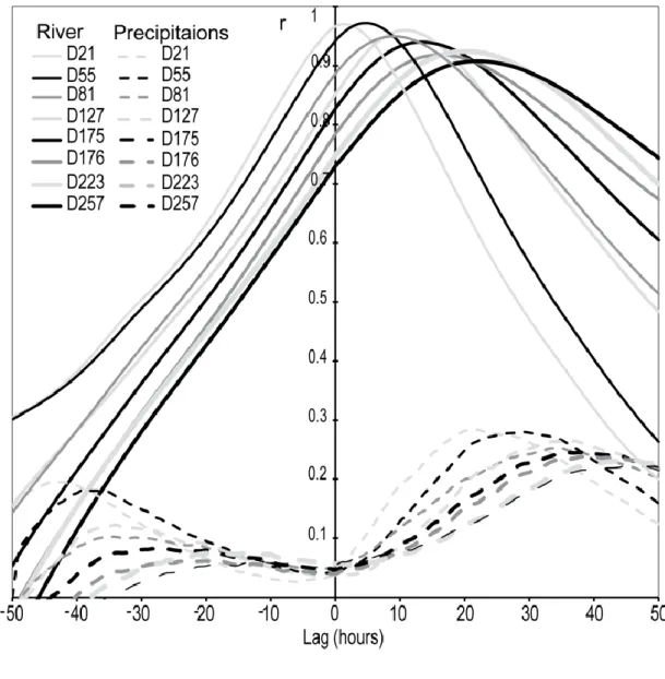
Figure 3 presents cross-correlation functions between river levels as input processes and 217
groundwater levels as output processes as well as cross-correlation functions between 218
precipitation and groundwater levels for the 2–16 July event. The results reflect the 219
strong relationship (r > 0.9 at maximum correlation) between the river stage fluctuations 220
and the groundwater level fluctuations at every piezometer. With values ranging from 221
0.89 to 0.98, and 8 correlations out of 11 being higher than 0.95, the cross-correlation 222
results suggest that groundwater levels are strongly correlated with river stage 223
fluctuations. The precipitation–groundwater level correlations (0.2 - 0.3) are significantly 224
lower than the river–groundwater level correlations. This gives strong evidence that the 225
input signal from precipitation is significantly reduced by the large storage capacity of 226
the unsaturated zone. 227
228
Time lags between inputs and outputs derived from the cross-correlation analysis reveal 229
the spatiotemporal response of the groundwater level to the rising stream discharge or to 230
the precipitation. For the 2–16 July event, time lags between precipitation and 231
groundwater levels (at maximum correlation) varied from 22 to 44 hours while time lags 232
between river stage and groundwater levels varied from 1 to 22 hours. In both cases, the 233
shorter time lags are associated with piezometers located closer to the river. The longer 234
precipitation-groundwater level time lags reveal a significant storage capacity of the 235
unsaturated zone during precipitation, and the shorter river-groundwater level time lags 236
are interpreted as an indication that groundwater fluctuations are associated with river 237
level fluctuations. 238
239
Figure 4 shows the relationship between the time lags from the river level-groundwater 240
level cross-correlation analysis and the piezometer distance from the river for three flood 241
events. A strong linear relationship emerges between the two variables as shown by the 242
strong R2 for the regression model for the three flood events (all R2 values are higher than 243
0.91). The scatter for each event may be due to the fact that the piezometers are not 244
perfectly aligned (see Figure 1c). The figure also shows that at 250 m the highest 245
groundwater level is reached 25 h later than the highest river stage for the September 246
flood event, but 40 h later for the November flood event. This reveals contrasting 247
propagation velocities for the groundwater crest moving throughout the floodplain. An 248
average propagation velocity can be estimated from the slope coefficient of the regression 249
lines. For the selected flood events, the propagation velocities range between 6.7 m h-1 250
and 11.5 m h-1. It can be noted that the two largest floods present a similarly high 251
propagation velocity while the lowest flood is linked with the smallest propagation 252
velocity. 253
254
The relative homogeneity of hydraulic conductivities over the floodplain shows that the 255
spatial distribution of lag values over the study site cannot be caused by floodplain 256
morphology. Comparison of hydraulic conductivity values to the floodplain elevation 257
(Table 1) also shows that spatial distribution of hydraulic conductivities is not explained 258
by the floodplain morphology. Moreover, if direct groundwater recharge or hillslope 259
runoff processes were responsible for groundwater level fluctuations, a large variability 260
of lag values among piezometers would not be obtained for every flood event. Relations 261
between time lags and peak stream discharge values and between time lags and rising 262
limb times were investigated and no significant relationships emerged. 263
The high correlation values, the short positive time lags, and the increasing time lags with 265
distance from the river observed from the cross-correlation analysis all suggest that 266
piezometric levels in the floodplain are controlled by river stage fluctuations. However, 267
this general pattern is variable in time and space. Figure 5 shows that there is a positive 268
correlation between the time lag and the day of the year (DOY) on which the flood event 269
occurred at four locations within the alluvial floodplain. The smallest time lags were 270
recorded for the summer flood events (DOY 188 to 249). For all piezometers, a 50% 271
increase in time lags between DOY 188 (7 July) and 336 (2 December) was observed. 272
Although there is a general tendency to the increase of time lag throughout the summer, 273
there is an opposite trend when several floods follow a period without precipitation event. 274
Two “dry” periods occurred during this study, between DOY 205 and 230, and between 275
DOY 250 and 320. For both periods, the first flood event has a significantly larger time 276
lag and the time lag for each of the following storm events occurring after was relatively 277
smaller. These “dry” periods resulted in a deeper unsaturated zone, which explain the 278
significant increased time lags followed by decreased time lag. 279
The amplitude of groundwater fluctuations decreased with distance from the river 280
(Figure 6). A damping effect can been seen, probably induced by the distance between 281
the piezometer and the channel. All R2 values are higher than 0.92. This amplitude 282
variability is not related to floodplain morphology. Comparing the three flood events 283
revealed that amplitudes conserve similar proportions, e.g., water level amplitudes 284
recorded at 21 m distance were always 60% higher than amplitudes recorded 250 m from 285
the channel, regardless of flood magnitude. In addition, the amplitudes of groundwater 286
fluctuations close to the channel can be higher than the amplitudes of river stage 287
fluctuations. For example, 21 m from the channel, the 0.37 m river level fluctuation 288
recorded during the 26 August–3 September event and the 1.04 m river level fluctuation 289
recorded during the 5–12 September event induced groundwater fluctuations of 0.40 m 290
(108%) and 1.14 m (109%), respectively. Also, comparison of the 26 August – 3 291
September event to 2–16 Julyeventshows that a flood event of a lower magnitude (0.37 292
m) and of a shorter rising limb (32.5 h) induces larger water level fluctuations than a 293
flood event of a higher magnitude (0.42 m) with a longer rising limb (90.8 h). The 294
amplitudes of groundwater fluctuations depend not only on the piezometer-channel 295
distance and on the magnitude of the flood events, but also on the duration of the flood 296
rising limb. 297
298
3.2 Spatial analysis of groundwater level dynamics 299
At the study site, the Matane River is generally a gaining stream, i.e., the hydraulic 300
gradient indicates that flow is towards the river. To investigate if the spatial dynamics of 301
hydraulic gradients is affected during a flood event, hourly groundwater equipotential 302
maps were produced. These maps suggest that hydraulic gradients vary temporally and 303
spatially during flood events and that they may reverse. Figure 7 shows that the water 304
pressure exerted on the channel banks from stream flooding induced hydraulic gradient to 305
change flow orientation during the 5–12 Septemberflood. At 22 m3 s-1 on 5 September at 306
00:00 am (Figure 7a), the Matane River was a gaining stream. The highest water level of 307
59.20 m at piezometer D223 and the lowest water level of 58.37 m at piezometer D21 308
indicate a west-oriented flow related to a hydraulic gradient of 3.31 mm m-1. The 309
hydraulic gradient indicated groundwater flow re-oriented towards the eastern valley 310
walls (Figure 7b) from 6 September 07:00 am (105 m3 s-1) to 11:00 pm (187 m3 s-1), even 311
if the peak stream discharge of 213 m3 s-1 was at 02:00pm. Using hydraulic heads from 312
piezometers D55 and D176, the steepest perpendicular hydraulic gradient obtained is 313
1.9 mm m-1 and been recorded at 3:15 pm on 6 September. The hydraulic gradient 314
returned to its initial orientation, i.e., gaining stream, at approximately 1:00pm on 7 315
September (Figure 7c). At that time, the hydraulic gradient between D223 and D21 was 316
2.81 mm m-1 and it is only on 8 September at 07:45 am that the hydraulic gradient at the 317
field site returned to its pre-storm condition of 3.31 mm m-1. 318
319
Based on the highest saturated soil hydraulic conductivity (8.48×10⁻⁴ m s-1, piezometer 320
D139 (table 1)), with the highest hydraulic gradient of 1.98 mm m-1 (observed at 3:15 pm 321
on 6 September), and a typical value of 0.25 for the effective porosity (Freeze and 322
Cherry, 1979), groundwater flow velocity through the floodplain during the inverted 323
hydraulic gradient was 2.41×10⁻² m h-1. However, cross-correlation analyses for the 5–12 324
September flood event indicate an average propagation velocity of 11.5 m h-1, i.e., two to 325
three orders of magnitude higher than the estimated groundwater velocity. This suggests 326
that hydraulic head fluctuations correspond to the propagation of a groundwater 327
floodwave throughout the floodplain triggered by the river stage fluctuation. The 5–12 328
September 213 m3 s-1 flood event is the only recorded event that induced a change in 329
groundwater flow orientation of the alluvial aquifer during the study period. However, it 330
is expected that larger flood events would induce similar processes. 331
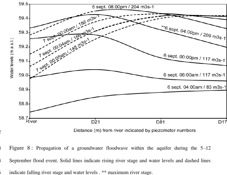
In order to evaluate the floodwave propagation through the Matane river alluvial aquifer, 333
hydraulic heads profiles from the stream through a transect of piezometers (D21, D81, 334
and D176) during the 5-12 September flood were assessed throughout the duration of the 335
flood (Figure 8). River levels used for the profiles come from the river stage gauge 336
downstream (RSGdn) temporal series. Results indicate that as the stage in the river 337
increased, the flow direction in the aquifer reversed. At the start of the flood pulse, 338
Matane river is a gaining stream. At the peak of the flood pulse on 6 September 04:00pm, 339
the groundwater flow orientation was towards the valley wall, indicating that the river 340
water level was higher than that of the alluvial aquifer. As the flood pulse receded, the 341
groundwater flow direction reverted back towards the stream. It should also be noted, that 342
as the river stage started to fall from 6 September 08:00pm to 7 September 04:00am, the 343
underground floodwave was still propagating through the floodplain, hydraulic gradient 344
was still reversed and hydraulic heads kept rising at D81 and D176. This would, first, 345
inform that a floodwave may propagates beyond the study site (> 250 m from the river), 346
but also highlight that the floodplain has stored water almost to the exfiltration of the 347
water table at the floodplain surface at D176 (59.51 m (Table 1)). It is finally on 7 348
September at 08:00 am that both river stage and water levels were falling. 349
350 351
4. DISCUSSION 352
4.1 Groundwater floodwave propagation 353
This study highlights the effects of the Matane River discharge fluctuations on the water 354
level of its alluvial aquifer. Field measurements suggest that a floodwave propagates 355
through the gravelly floodplain over a spatial extent much larger than the hyporheic zone. 356
Results also suggest that the alluvial aquifer of the Matane Valley is hydraulically 357
connected and primarily controlled by river stage fluctuations, even at stream discharges 358
below bankfull. It has been reported that river stage fluctuations in some catchments were 359
the processes primarily responsible for groundwater fluctuations throughout a floodplain 360
(Lewandowski et al., 2009; Vidon, 2012). Another study reports that piezometers distant 361
from the channel reflect hillslope groundwater contributions (Jung et al., 2004). Here, 362
cross-correlation results (Figure 3b) show lower correlations and much longer delays 363
between precipitation and groundwater levels than between river levels and groundwater 364
levels. It is clear that direct precipitation contributes to recharge the unconfined alluvial 365
aquifer. However, this is not the primary process responsible for groundwater increases 366
during the flood events, probably because of the unsaturated storage capacity. 367
Lewandowski et al. (2009) showed that precipitation was responsible for 20% of the 368
groundwater fluctuations in the River Spree floodplain whereas, Vidon (2012) noted also 369
no significant correlation between precipitation and groundwater fluctuations, 370
371
The propagation of the hydraulic head fluctuations through alluvial aquifers during flood 372
events has been discussed by several authors (Sophocleous, 1991; Jung et al., 2004; 373
Lewandowski et al., 2009; Vidon, 2012). Jung et al. (2004) compared their results to a 374
kinematic wave propagation based on flux velocities. This was done on a nearly 375
synchronous response of the groundwater to the river stage during in-bank conditions, 376
and on a wave-like response of the groundwater induced by an increase in river stage. 377
Kinematic wave theory (see Lighthill and Withman, 1955) is based on the law of mass 378
conservation through the continuity equation and a flux-concentration and may be 379
applicable over a wide range of hydrological processes (Singh, 2002). To be considered 380
as kinematic, a wave must be nondispersive and nondiffusive, two conditions that are 381
necessary for the conservation of its length and amplitude over time and throughout 382
space. In contrast, Thual (2008) showed that a dispersive and diffusive wave is 383
considered as a dynamic wave. The amplitude of a dynamic wave will decrease over time 384
and throughout space, but its length will increase. 385
386
In this study, the propagation of an underground floodwave, triggered by the river stage 387
fluctuations for all flood events, is interpreted as a dynamic wave propagating within the 388
alluvial aquifer. This interpretation is based on the non-conservation of hydraulic head 389
fluctuations over time and through space. The groundwater response to the pulse induced 390
by the rising river stage is however delayed and damped through the floodplain, as noted 391
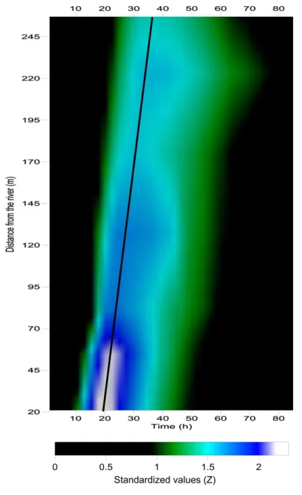
in Vekerdy and Meijjerink (1998) and Lewandowski et al. (2009). Figure 9 is a 392
representation of a dynamic wave propagation through the alluvial aquifer of the Matane 393
floodplain for the 5–12 September flood event. Near the river, hydraulic head amplitudes 394
are high but the duration of high hydraulic heads is short. As a groundwater floodwave 395
propagates distant from the river, friction through the porous medium causes a loss of 396
energy, which induces the damping effect. This damping effect causes water table 397
amplitudes to become smaller, but hydraulic heads to remain high longer, inducing the 398
floodwave crest to migrate (Figure 9). Every flood event, independent of its magnitude, 399
induced dynamic wave propagations, but it is only the September event that caused 400
hydraulic gradient to change flow orientation. 401
402
The groundwater floodwave hypothesis is also supported by the fact that a streamflood 403
event induces water levels to rise instead of creating a lateral groundwater mass 404
displacement through the floodplain. The absence of a significant displacement of river 405
water in the floodplain during a flood event is supported by the propagation velocities of 406
the 5–12 September flood event that are 2-3 orders of magnitude higher (6.00 to 10.93 407
m h-1) than the groundwater velocity (10-2 m h-1) measured at the highest reversed 408
hydraulic gradient of the field site (1.9 mm m-1) on 6 September at3:15 pm. These results 409
support those of Vidon (2012), who reported propagation velocities three orders of 410
magnitude higher than groundwater velocities, which were in the range of 10-4 m h-1. 411
Jung et al. (2004) reported propagation velocities five to six orders higher than flux 412
velocities of 10-4-10-5 m h-1,whereas Lewandowski et al. (2009) noted the propagation of 413
pressure fluctuations approximately 1000 times faster than groundwater flow. Figure 5 414
shows an increase in the time lag throughout the year induced by a long period of 415
groundwater discharging to the river between the 5–12 September and the 10–26 416
November flood events. This increase in the time lag represents not only a reduction of 417
propagation velocities through the year, but also highlights the effects of prior 418
unsaturated zone. Propagation velocities are not correlated with rainfall intensity. If 419
rainfall intensity affected time lags, a large variability of time lags between piezometers 420
would not be observed at each flood event, nor would it be observed for similar rainfall 421
intensities. 422
423
Streamfloods can affect the local groundwater flow directions in the floodplain 424
depending on the flood magnitude. Potentiometric maps (Figure 7) show that the 425
hydraulic gradient within the floodplain reversed at a stream discharge of 95 m3 s-1 during 426
the 5–12 September flood event. Some researchers have reported reversed hydraulic 427
gradients and the development of a groundwater ridge toward valley walls capable of 428
‘swiching off’ hillslope inputs during a streamflood with a stream discharge below 429
bankfull, sometimes for long periods (e.g. Burt et al., 2002; Vidon, 2012). Here, the 5–12 430
September event is the only event that induced a groundwater flow reversal which lasted 431
16 h before returning to pre-storm initial hydraulic gradient three days later. 432
433
4.2 Groundwater flooding 434
The occurrence of groundwater flooding in floodplain environments is controlled by the 435
degree of connectivity between a stream and its alluvial aquifer (Mardhel et al., 2007; 436
Cobby et al., 2009). Figure 8 shows that groundwater levels rise almost synchronously as 437
the river stage rises. But to determine the range of stream discharges at which exfiltration 438
is likely to occur at study site, linear regression analyses for each piezometer were 439
calculated using highest hydraulic heads reached below floodplain surface and the peak 440
flow of recorded flood events (Figure 10a). Strong correlations (R 2> 0.96) exist for all 441
piezometers, taking account the 213 m3 s-1 event or not. For example, the 213 m3 s-1 442
during the 5–12 September event induced the hydraulic head to rise to 9 cm below the 443
surface at D176 and to 15 cm below the surface at D21 and D81. The hydraulic heads 444
rose closest to the floodplain surface at piezometers installed in the oxbow feature. 445
Figure 10b shows the spatial distribution of the predicted stream discharges producing 446
exfiltration at the study site. By extrapolating from the water level depths-flowrates 447
relations, it is possible to estimate that exfiltration would occur at stream discharges 448
ranging between 238 and 492 m3 s-1 depending on the location within the floodplain. 449
Figure 10b shows that the lowest predicted stream discharges would induce flooding at 450
the lowest part of the floodplain (i.e., in the oxbow), and at piezometers D55 and D175 451
only stream discharges higher than bankfull would induce exfiltration of the water table. 452
Estimated bankfull discharge of the Matane River is 350 m3 s-1, so according to the 453
models, exfiltration occurs at stream discharges well below bankfull. The range of stream 454
discharges that took place during the study period were all below the extrapolated 455
exfiltration thresholds supporting the fact that no exfiltration event was observed. 456
Although the exfiltration thresholds would need validation, the data strongly indicate that 457
river stage levels and underground floodwave propagation can contribute to groundwater 458
flooding. Further developments in the estimation of groundwater flooding river flow rates 459
should consider the initial hydraulic heads before stream floods occurred, the spatial 460
connectivity between piezometers by runoff at the floodplain’s surface once exfiltration 461
occurred, or a possible overflow of the Matane River. 462
463
5. CONCLUSION 464
This study shows that water level fluctuations in the Matane alluvial floodplain are 465
primarily governed by river stage fluctuations. The amplitudes of groundwater 466
fluctuations depend on the distance from the channel, on the flood magnitude, and on the 467
rising limb of the flood. The largest flood event recorded during the study period is the 468
only event that influenced local groundwater flow orientation within the alluvial 469
floodplain by generating an inversion of the hydraulic gradient toward the valley walls 470
for sixteen hours. The results also show a damping effect of the groundwater response 471
related to the distance of piezometers from the channel. Every flood event showed a large 472
variability of lag values across the floodplain. The periods of groundwater discharging to 473
the river of july and October 2011 caused time lags to increase for next flood events. 474
Exfiltration of groundwater is predicted for stream discharges that can be well below 475
bankfull. However, these estimations do not take into account the spatial connectivity 476
between piezometers, the initial depth of the groundwater, or a possible overflow of the 477
river. Finally, this study reveals that the pressure exerted on the river bank by a stream 478
flood induces the propagation of a groundwater floodwave, interpreted as a dynamic 479
wave, for all the studied floods. The propagation speed remains relatively constant across 480
the floodplain but depends on the initial conditions within the floodplain. Propagation of 481
groundwater level fluctuations occurs at every event, but only the largest event in this 482
study affected groundwater flow directions. This study supports the idea that a river flood 483
has a much larger effect in time and space than what is occurring within the channel. 484
Further research including groundwater geochemistry would bring insights on energy 485
exchange processes through the river bank and allow to determine whether and to what 486
distance surface water reaches the floodplain below ground the during flood events. 487
488
ACKNOWLEDGEMENTS 489
This research was financially supported by the climate change consortium Ouranos as 490
part of the “Fonds vert” for the implementation of the Quebec Government Action Plan 491
2006-2012 on climate change, by BORÉAS, by the Natural Sciences and Engineering 492
Research Council of Canada (NSERC), by the Centre d’Études Nordiques, and by the 493
Fondation de l’UQAR. We are thankful to several team members of the Laboratoire de 494
recherche en géomorphologie et dynamique fluviale de l’UQAR for field assistance. 495
REFERENCES 497
Barlow, J.R., Coupe, R.H., 2009. Use of heat to estimate streambed fluxes during 498
extreme hydrologic events. Water Resour. Res. 45 (1), 1-10,doi: 566 499
10.1029/2007WR006121. 500
Burt, T.P., Bates, P.D., Stewart, M.D., Claxton, A.J., Anderson, M.G., Price, D.A., 2002. 501
Water table fluctuations within the floodplain of the River Severn, England. J. Hydrol. 502
262 (1–4), 1–20. 503
Cardenas, M.B., 2008. The effect of river bend morphology on flow and timescales of 504
surface water-groundwater exchange across pointbars. J. Hydrol. 362 (1–2), 134–141. 505
Cobby, D., Morris, S., Parkes, A., Robinson, V., 2009. Groundwater flood risk 506
management: advances towards meeting the requirements of the EU floods directive. J. 507
Flood Risk Manag. 2 (2), 111–119. 508
Freeze, R.A., Cherry, J.A., 1979. Groundwater. Prentice Hall, Englewood Cliff. 509
Gillham, R.W., 1984.The capillary fringe and its effect on water-table response. J. 510
Hydrol. 67, 307–324. 511
Gooseff, M.N., 2010. Defining hyporheic zones – Advancing our conceptual and 512
operational definitions of where stream water and groundwater meet. Geo. Compass 4 513
(8), 945–955. 514
Haycock, N.E, Burt, T.P., 1993. Role of floodplain sediments in reducing the nitrate 515
concentration of subsurface run-off : a case study in the Cotswolds, UK. Hydrol. 516
Processes 7, 287-295. 517
Hammer, Ø., Harper, D.A.T., Ryan, P.D., 2001. PAST: Paleontological statistics 518
software package for education and data analysis. Palaeontologia Electronica , 4 (1), 9. 519
Harvey, J.W., Bencala, K.E., 1993. The effect of streambed topography on surface– 520
subsurface water exchange in mountain catchments. Water Resour. Res. 29 (1), 89–98, 521
doi: 10.1029/92WR01960. 522
Harvey, J. W., J. D. Drummond, R. L. Martin, L. E. McPhillips, A. I. Packman, D. J. 523
Jerolmack, S. H. Stonedahl, A. Aubeneau, A. H. Sawyer, L. G. Larsen, and C. Tobias, 524
2012, Hydrogeomorphology of the hyporheic zone: Stream solute and fine particle 525
interactions with a dynamic streambed. J. Geo. Res. - Biogeosciences, Volume 117, 526
G00N11, doi:10.1029/2012JG002043. 527
Hvorslev, M.J., 1951. Time lag and soil permeability in groundwater observation. U.S. 528
Army Corps of Engineers, Waterways Experimental Station, Vicksburg, Miss., Bulletin 529
365. 530
Jung, M.T., Burt, T.P., Bates, P.D., 2004. Toward a conceptual model of floodplain water 531
table response. Water Resour. Res. 40 (12), 1–13. 532
Kreibich, H., Thieken, A., 2008. Assessment of damage caused by high groundwater 533
inundation. Water Resour. Res. 44 (9), W09409, doi:10.1029/2007WR006621. 534
Lebuis, J., 1973. Geologie du Quaternaire de la region de Matane-Amqui- Comtes de 535
Matane et de Matapedia. Rapport DPV-216, Ministere des Richesses naturelles, Direction 536
generale des Mines, Gouvernement du Quebec, Quebec, 18. 537
Lewandowski, J., Lischeid, G., Nützmann, G., 2009. Drivers of water level fluctuation 538
and hydrological exchange between groundwater and surface water at the lowland river 539
Spree (Germany): field study and statistical analyses. Hydrol. Processes 23 (15), 2117– 540
2128. 541
Lighthill M.J., Whitham, G.B., 1955. On kinematic waves: 1. Flood movement in long 542
rivers. Proceedings of the Royal Society London, Series A 229, 281–316. 543
Mardhel, V., Pinault, J.L., Stollsteiner, P., Allier, D., 2007. Etude des risques 544
d’inondation par remontees de nappe sur le bassin de la Maine, Rapport 55562-FR, 545
Bureau de recherches geologiques et minieres, 156. 546
Mertes, L.A., 1997. Documentation and significance of the perirheic zone on inundated 547
floodplains. Water Resour. Res. 33 (7), 1749–1762. 548
Pinault, J.L., Amraoui, N., Golaz, C., 2005. Groundwater-induced flooding in macropore-549
dominated hydrological system in the context of climate changes. Water Resour. Res. 41 550
(5), 1–16. 551
Singh, V.P., 2002. Is hydrology kinematic? Hydrol. Processes, 16 (3), 667–716. 552
Sophocleous, M.A., 1991. Stream-floodwave propagation through the great bend alluvial 553
aquifer, Kansas: Field measurements and numerical simulations. J. Hydrol. 124 (3–4), 554
207–228. 555
Stonedahl, S.H., Harvey, J.W., Wörman, A., Salehin, M., Packman, A.I., 2010. A 556
multiscale model for integrating hyporheic exchange from ripples to meanders. Water 557
Resour. Res. 46, 1–14,doi:10.1029/2009WR008865. 558
Thual, O., 2008. Propagation de l’onde de crue, in Thual, O. (Ed.), Hydrodynamique de 559
l’Environnement. Les Editions de l’Ecole Polytechnique, Toulouse, pp.131-157. 560
Triska, F.J., Kennedy, V.C., Avanzio, R.J., Zellweger, G.W., Bencala, K.E., 1989. 561
Retention and transport of nutrients in a third-order stream in northwestern California: 562
Hyporheic processes. Ecology, 70 (6), 1893–1905. 563
Vekerdy, Z., Meijerink, A.M.J., 1998. Statistical and analytical study of the propagation 564
of flood-induced groundwater rise in an alluvial aquifer. J. Hydrol., 205 (1–2), 112–125. 565
Vidon, P., 2012. Towards a better understanding of riparian zone water table response to 566
precipitation: surface water infiltration, hillslope contribution or pressure wave 567
processes? Hydrol. Processes, 26 (21), 3207–3215. 568
Woessner, W., 2000. Stream and fluvial plain interactions: rescaling hydrogeologic 569
thought. Groundwater, 38 (3), 423–429. 570
Wondzell, S.W., Gooseff, M.M., 2013, Geomorphic controls on hyporheic exchange 571
across scales: watersheds to particles, in Shroder, J. F. (Ed.), Treatis in Geomorphology. 572
Academic Press, San Diego, pp. 203-218. 573
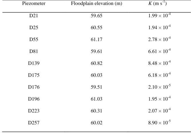
Table 1: Hydraulic conductivity values derived from slug tests. 575
Piezometer Floodplain elevation (m) K (m s-1)
D21 59.65 1.99 × 10⁻⁴ D25 60.55 1.94 × 10⁻⁴ D55 61.17 2.78 × 10⁻⁴ D81 59.61 6.61 × 10⁻⁴ D139 60.82 8.48 × 10⁻⁴ D175 60.03 6.18 × 10⁻⁴ D176 59.51 2.10 × 10⁻⁵ D196 61.03 1.95 × 10⁻⁴ D223 60.31 2.07 × 10⁻⁴ D257 60.02 8.90 × 10⁻⁵ 576 577
578
579
Figure 1 : (A) Location of the the Matane River Basin, Quebec, Canada; (B) Location of 580
the study site within a coarse sand gravelly floodplain constructed by fluvial dynamics; 581
(C) Position of the piezometers within the study site. Piezometers with pressure sensors 582
are indicated. The names of the piezometers reflect the perpendicular distance to the 583
Matane River. 584
586
Figure 2 : Water levels and river stage time series from 21 June to 12 December 2011. 587
589
Figure 3 : Cross-correlation functions using river levels as input and groundwater levels 590
as output (solid lines) and precipitation as input and groundwater levels as output (dashed 591
lines). 592
594
Figure 4 : Time lags of piezometers as a function of distance from the river for three 595
selected flood events. 596
598
Figure 5 : Time lags as a function of day of the year of flood occurrence at four selected 599
positions within the alluvial floodplain. 600
602
603
Figure 6 : Water level fluctuations within the floodplain for three flood events. Values 604
parenthesis indicate duration of flood pulse rising limb and flood even magnitude. 605
607
Figure 7 : Groundwater flow directions suggested from the equipotential lines during 5– 608
12 September event. 609
611
612
Figure 8 : Propagation of a groundwater floodwave within the aquifer during the 5–12 613
September flood event. Solid lines indicate rising river stage and water levels and dashed lines 614
indicate falling river stage and water levels . ** maximum river stage. 615
617
Figure 9 : Floodwave propagation within the floodplain for the 5–12 September 213 m3s-1 618
flood event using the standardized water level from pieozometers D21, D55, D81, D127, 619
D175, D223 and D257. Step time is hourly from 6 September, 00:00 am. The black line 620
represents the groundwater floodwave crest displacement. 621
622
Figure 10 : Predicted stream discharges for exfiltration. (a) Regression model of 623
predicted exfiltration discharge for selected piezometers; (b) spatial distribution of the 624
predicted exfiltration discharges. Regression dashed lines correspond to extrapolation. 625
Vertical dashed line correspond to Matane river bankfull discharge. 626