HAL Id: hal-01852327
https://hal-mines-albi.archives-ouvertes.fr/hal-01852327
Submitted on 1 Aug 2018
HAL is a multi-disciplinary open access
archive for the deposit and dissemination of
sci-entific research documents, whether they are
pub-lished or not. The documents may come from
teaching and research institutions in France or
abroad, or from public or private research centers.
L’archive ouverte pluridisciplinaire HAL, est
destinée au dépôt et à la diffusion de documents
scientifiques de niveau recherche, publiés ou non,
émanant des établissements d’enseignement et de
recherche français ou étrangers, des laboratoires
publics ou privés.
BRDF (Bidirectional Reflectivity Distribution Function)
modelling for accuracy enhanced thermoreflectometry
Benjamin Javaudin, Rémi Gilblas, Thierry Sentenac, Yannick Le Maoult
To cite this version:
Benjamin Javaudin, Rémi Gilblas, Thierry Sentenac, Yannick Le Maoult. BRDF (Bidirectional
Re-flectivity Distribution Function) modelling for accuracy enhanced thermoreflectometry. QIRT 2018
- 14th Quantitative InfraRed Thermography Conference, QIRT, Jun 2018, Berlin, Germany. 9 p.,
�10.21611/qirt.2018.123�. �hal-01852327�
BRDF (Bidirectional Reflectivity Distribution Function) modelling for accuracy
enhanced thermoreflectometry
by B. Javaudin*, R. Gilblas*, T. Sentenac*, Y. Le Maoult*
*Institut Clément Ader (ICA), Université de Toulouse, CNRS, IMT Mines Albi, UPS, INSA, ISAE-SUPAERO, Campus Jarlard, 81013 Albi CT Cedex 09, France, [email protected]
Abstract
In the field of thermography, the main problem of measuring the true temperature is the knowledge of the emissivity. Thermoreflectometry overcomes this problem by including an “in-situ” emissivity determination based on bidirectional reflectivity measurement. However, this method introduces an unknown diffusion function in order to link this measurement to the emissivity. The suggested modelling of this function is based on physical models of Bidirectional Reflectivity Distribution Function (BRDF). The model is then compared with the experimental BRDF of a platinum sample and the diffusion function is studied as a function of the roughness and for two geometrical configurations.
Nomenclature
𝜀𝑥 Directional emissivity Ω𝑥 Solid angle in direction x, [𝑠𝑟]
𝜌𝑥,∩ Directional hemispherical reflectivity 𝐿𝑥 Unit vector in the direction x
𝜌𝑖,𝑟 Bidirectional reflectivity, [𝑠𝑟−1] 𝑁, 𝐻 Unit normal vector global and local
𝜂𝑟,𝑖 Diffusion function, [𝑠𝑟] Indexes and exponents
𝑓𝜆0 Normal specular reflectivity 𝑖, 𝑟, 𝑥 Light source, detector and variable directions
𝑚 Standard deviation of slopes ∩, 𝜆 Hemispherical quantity and spectral quantity
1. Introduction
Temperature is a key parameter in many industrial processes and its measurement by non-contact techniques like thermography offer many advantages compared to contact techniques. This method has the capability to provide radiance temperature measurement but it requires the knowledge of the surface emissivity to compute the true temperature. The emissivity can be taken into account following two approaches: passive and active thermography.
Passive thermography minimises the impact of the lack of the emissivity knowledge by operating the camera in the ultraviolet band [1]. Polychromatic thermography [2] spectrally models the behaviour of the emissivity and solves a system composed by the spectral radiometric equations. Then, the temperature and the parameter(s) of the emissivity model are estimated. This method assumes that the variation of the emissivity is consistent with the modeling during all the time of the experiment. However, the assumption can be quickly obsolete because of the evolution of the surface state due to oxidation phenomena.
Active thermography overcomes the emissivity change problem by including an “in-situ” emissivity determination. For instance, thermoreflectometry [3,4] suggests an indirect measurement of emissivity based on bidirectional reflectivity measurement. However, for an opaque material, directional emissivity is linked to directional-hemispherical reflectivity by Kirchhoff’s law. Thermoreflectometry then introduces a relationship between those two quantities through an unknown function, called the diffusion function. The remaining problems are: 1- the modelling of the diffusion function in relation to the material; 2- the optimisation of the number of wavelength according to the dependence of the diffusion function modelled.
This article aims to model the diffusion function thanks to the physical model of Bidirectional Reflectivity Distribution Function (BRDF). The BRDF gives the opportunity to include in the diffusion function the surface properties of the material (roughness and optical index of refraction) and also the geometrical measurement settings. The suggested approach of modelling is based on the micro-facet theory applied in geometric optic. The BRDF is then the sum of elementary specular reflections on micro-facets, which orientations are statistically described. The first part of the article will be devoted to the introduction of the diffusion function. The second part will present a model of the diffusion function based on micro-facet approach. Finally the model of BRDF will be compared to a measurement of the BRDF on a platinum sample. The diffusion function will be computed versus the roughness and the measurement settings. This model will be also compared with an experimental identification of the diffusion function by bi-chromatic thermoreflectometry.
14
thQuantitative InfraRed Thermography Conference, 25 – 29 June 2018, Berlin, Germany
2
2. Introduction of the diffusion function in thermoreflectometry
Thermoreflectometry is based on the radiometric equation which links the measured radiance to the Planck’s law. Thus, a thermal emission recorded by a camera can be converted into a temperature called radiance temperature. For a black body, this temperature is also the true temperature. For common bodies, the true temperature can be deduced from the radiance temperature only if the directional emissivity (𝜀𝜆𝑟) in the right spectral band is known.
Thermoreflectometry suggests an indirect determination of the emissivity. For an opaque material and thanks to the Kirchhoff’s laws, the directional hemispherical reflectivity measurement is required to deduce the emissivity. The thermoreflectometry only measures the bidirectional reflectivity (𝜌𝜆𝑖,𝑟) and introduces an unknown diffusion function (𝜂
𝜆 𝑟,𝑖)
to deduce the emissivity. Following the Kirchhoff’s law, theses quantities are linked by the following equation:
, , ,
1
1
r r r i i r
(1)Where the exponent r is the direction of the detector, i the direction of the light source and ᴖ represents the half-hemisphere up to the surface. The unit of 𝜂𝜆𝑟,𝑖 is then [𝑠𝑟] and 𝜌
𝜆
𝑖,𝑟 [𝑠𝑟−1].
This work aims at modelling a diffusion function that takes physically into account the reflective behaviour of the material. It involves modelling a more general quantity: the Bidirectional Reflectivity Distribution Function (BRDF). This function includes the directional reflectivity of a surface in all the geometries possible. From Eq. (1), the diffusion function is then directly linked to the BRDF by:
, , , 2 , ,
cos
x r x x x r r i i r i rd
(2)Where 𝑑Ω𝑥 is the solid angle in the direction x and forms an angle 𝜃𝑥 with the surface normal. The directions i
and r are fixed quantities and x takes all the values in the half hemisphere Ω = 2𝜋.
Eq. (2) shows that for a given surface and a given detector direction (𝑟), the diffusion function depends on the direction of the light source (𝑖). Thus, the behaviour of the diffusion function depends on the choice of the geometrical settings (𝑟, 𝑖), in addition to the surface properties included in the BRDF. Modelling the diffusion function is then an opportunity to know the sample properties and the best measurement setting. In the next section, a BRDF model will be presented and expressed in the directions (𝑖, 𝑟) and (𝑟, 𝑥) in order to deduce the diffusion function of the Eq. (2).
3. Modelling the diffusion function from a BRDF model
3.1. Choice of a BRDF model
The BRDF is a function that defines how light is reflected by an opaque surface from an incoming light direction to an outgoing direction. For a given configuration (𝑖, 𝑟), a global coordinate system, showed on figure 1, is defined from the normal vector (𝑁) of the surface. The vector (𝐿𝑖) defines the direction of the incoming light and (𝐿𝑟) the outgoing
direction. These two vectors define with (𝑁) the zenith angles noted 𝜃𝑖 and 𝜃𝑟. Finally, the azimuth angle 𝜙, between the
projection of 𝐿𝑖 and 𝐿𝑟 on the plane of the surface (which normal vector 𝑁) generalizes the definition of this global
geometry in all the hemisphere. As a remark, the definition of 𝜙 defines a rotational symmetry of (𝐿𝑖, 𝐿𝑟) around the
normal vector. In that case, the BRDF model will also have this symmetry which is only true when the roughness does not depend on the sample orientation (isotropic roughness behaviour). The BRDF definition is then as following:
,
( ,
, )
r i r i r idL
dE
(3)Where 𝑑𝐿𝜆𝑟 is an elementary spectral radiance reflected and 𝑑𝐸𝜆𝑖 the elementary spectral irradiance.
The reflective behaviour of an opaque surface can be divided into two categories: the specular one which is described by the Fresnel model and the diffuse one which is described by the Lambert model. However, the modelling for diffuse surface is more complex and it is necessary to take into account the interaction between the light and the surface roughness. In order to describe the reflection process on the roughness, the geometric optic approximation, also called ray optic, will be used. This theory describes the light as a group of elementary rays which follow Fresnel equations. This choice, which neglects the wavelike behaviour of the light, involves that the size of the roughness is
10.21611/qirt.2018.123
much larger than the wavelength. Quantitative criteria on roughness parameters can be found in [5] which compares wave theory and geometric optic in the case of Gaussian random surfaces which will be used in the model later.
Torrance and Sparrow [6] combine the geometric optics with a statistic description of the roughness in a micro-facet BRDF model. Each bidirectional reflectivity of the BRDF is then the consequence of the sum of elementary Fresnel’s reflections on micro-facet oriented in defined position. Thus the shape of the BRDF becomes linked to the statistical distribution function of the micro-facets orientations. In addition to figure 1, a local frame, represented on figure 2, describes the reflection of the light on a micro-facet. 𝐻, is defined as the bisector vector of (𝐿𝑖, 𝐿𝑟). In this way, each
micro-facet oriented by an angle (𝛼), is settled to reflect the light from (𝐿𝑖, 𝐿𝑟). The angle of this specular geometry if then
noted 𝛽. Finally, for a given global geometry (𝜃𝑖, 𝜃𝑟, 𝜙), the Torrance model is expressed in Eq. (4).
Fig. 1. Global coordinate system with the units vector 𝐿𝑖, 𝐿𝑟, 𝑁 and the angles 𝜃𝑖, 𝜃𝑟, 𝜙
Fig. 2: Local coordinate system on a micro-facet with the local normal vector 𝐻, 𝐿𝑖 and 𝐿𝑟 in the
plane of the figure.
,
( ,
,
) ( ) ( ,
)
( ,
, )
4
cos
i r i r i r i rF
n k D
G
cos
(4)Where the angles (𝛼, 𝛽) are related to (𝜃𝑖, 𝜃𝑟, 𝜙) by the definition of the 𝐻 = 𝐿𝑖+𝐿𝑟
‖𝐿𝑖+𝐿𝑟‖. Also, the exponents (𝑖, 𝑟)
are switchable, which respects the reciprocity path theorem ( 𝜌𝜆𝑖,𝑟= 𝜌𝜆𝑟,𝑖).
The Fresnel function, 𝐹(𝛽, 𝑛𝜆, 𝑘𝜆), gives the specular reflectance of the materials in a case of an incident angle
𝛽. The angle of the micro-facet associated is then 𝛼. This function includes the spectral dependence of the BRDF with the complex index of refraction (𝑛𝜆, 𝑘𝜆) associated to the material.
The distribution function, 𝐷(𝛼), describes the amount of energy reflected by all the micro-facets oriented by the angle 𝛼. Thus, this function encompasses the topologic description of the surface in a probability distribution function with the random variable 𝛼.
Finally, the geometric attenuation factor function, 𝐺(𝜃𝑖, 𝜃𝑟), takes into account the shadowing and masking
effects, induced between the micro-facets. The shadowing arises when a micro-facet obstructs the path of the incoming light and the masking when the outgoing path is obstructed. However, these two geometrical effect are strong only for grazing angles and do not depend on the wavelength. Also they should be completed by a modelling of muli-reflection. Thus the function 𝐺 will be neglected in this first version of the BRDF model to keep the model simple.
3.2. Writing the diffusion function from a known bidirectional reflectivity
The diffusion function of Eq. (2) is rewritten according to the bidirectional reflectivity of Eq. (4) and the fixed angles (𝜃𝑖, 𝜃𝑟, 𝜙, 𝛼, 𝛽) for 𝜌
𝜆𝑖,𝑟 (and respectively the moving angles (𝜃𝑟, 𝜃𝑥, 𝜙𝑟,𝑥, 𝛼𝑟,𝑥, 𝛽𝑟,𝑥) for 𝜌𝜆𝑟,𝑥).
3.2.1 Bidirectional reflectivity expression
In Eq. (3), the distribution function, 𝐷(𝛼), is expressed with the distribution function of Beckmann [7], used also in the BRDF model of Cook-Torrance [8]. A Gaussian distribution of the slope of the micro-facets is considered. The slope is also the tangent of the angle 𝛼. The distribution is centred (average slope null) and the distribution’s shape depends only on the standard deviation of the slopes noted 𝑚. This function is detailed in Eq. (5).
14
thQuantitative InfraRed Thermography Conference, 25 – 29 June 2018, Berlin, Germany
4 2 , 2 , 2 4 ,tan
exp
2
(
, )
2
cos
r x r x r xm
D
m
m
(5)Where 𝛼𝑟,𝑥 depends on the vector 𝐿𝑟 and 𝐿𝑥 and it is noted 𝛼 for 𝐿𝑖 and 𝐿𝑟.
In Eq. (4), assuming that the angle 𝛽 stays close to zero, the Fresnel function, 𝐹(𝛽, 𝑛𝜆, 𝑘𝜆) is approximated by
the normal Fresnel factor 𝑓𝜆0 as follows:
2 2 0 2 2
(
1)
( ,
,
)
(
1)
n
k
F
n k
f
n
k
(6)Where 𝑛𝜆 is the refractive index and 𝑘𝜆 the imaginary part of the complex refractive index.
The benefit of this approximation is to replace the optical index by only one variable 𝑓𝜆0. Finally, according to Eq. (4), (5)
and (6), the two bidirectional reflectivities, 𝜌𝜆𝑖,𝑟and 𝜌 𝜆 𝑟,𝑥, become: 0 , , ,
( , )
,(
,
,
) (
, )
and
4
cos
4
cos
r x r x i r r x i r r xf D
m
F
n k D
m
cos
cos
(7)3.2.2 Diffusion function expression
According to Eq. (7), the diffusion function of Eq. (2) is rewritten as follows:
, , , 0 2
cos
( ,
,
)
(
,
,
) (
, )
( , )
x i r i r x r x xm n k
F
n k D
m d
f D
m
(8)For the experiment settings, , ,
/ 2
;
0°
/
2
4
5°
i r x r x x
, the Fresnel function 𝐹 in the integral can be also approximated by normal Fresnel factor 𝑓𝜆0. Indeed, with a detector aligned with the surfacenormal (𝐿𝑟= 𝑁 and 𝜃𝑟= 0°) and a light source close to the normal with an angle: 𝜃𝑖= 13° the symmetry around 𝑁
eliminates the need of the angle 𝜙.
That case restricts the range of 𝛽𝑟,𝑥 and thus only the micro-facets oriented with an angle below 45° contribute
in the BRDF. This means that a limit slope standard deviation is introduced, noted 𝑚𝑙𝑖𝑚, to guaranty the validity of the
approximation. Using normal Fresnel factor also in the integral part, the diffusion function of Eq. (8) becomes:
, , 2
cos
( )
(
, )
( , )
x i r i r x xm
D
m d
D
m
(9)For instance, a numerical application, presented below on the platinum with the refractive indexes taken from [8] (𝑛𝜆= 5.5 and 𝑘𝜆= 6.67 at 𝜆 = 2 𝜇𝑚), gives:
- 𝑓𝜆0≈ 𝐹(13°, 𝑛
𝜆, 𝑘𝜆) = 0.7461 and 𝐹(45°, 𝑛𝜆, 𝑘𝜆) = 0.7373 (1.18% relative error)
- 𝑚𝑙𝑖𝑚= 0.3 with a relative error below 0.1% between 𝜂𝜆𝑟,𝑖(𝑚) (Eq. (7)) and 𝜂𝜆𝑟,𝑖(𝑚, 𝑛𝜆, 𝑘𝜆) (Eq. (9))
With this approximation the diffusion function does not depend on the wavelength anymore. The only variable is the standard slope deviation 𝑚 which must be below a 𝑚𝑙𝑖𝑚 associated to the setting. Also, the limit found in the
numerical application allows a large range a surface finishes. In the following studies, the diffusion function of the Eq.(9) will be kept. An experimental study on a platinum sample will be presented.
10.21611/qirt.2018.123
4. Application of the model to a platinum sample
4.1. Measurement of the sample roughness
The behaviour of the BRDF is illustrated on a pure platinum sample (pure at 99.95%) with a controlled surface state. This metal was chosen because it slightly oxidates and its optical properties are well documented in the literature. The sample was sandblasted to obtain a non-specular and isotropic surface. The measurement of the roughness was performed on a confocal profilometer operating with white light.
The figure 3 presents a roughness profile of the sample with the detailed expression of the slope calculation which is the growth rate on each point of the profile. The standard-deviation (𝑚) associated to these slopes is also calculated and the formula is given Fig.4. The figure 4 shows the experimental distribution of slope normalized as a density probability function (the sum of the bar areas is one).
Fig. 3. Roughness profile of the platinum sample Fig. 4. Density probability of the slope and Gaussian model The experimental distribution of the slope is centred and follows a Gaussian distribution also plotted on Fig. 4. The Beckmann’s model chosen for modeling is therefore suitable for this sample. The next part is devoted to a comparison between the BRDF model and measurement on this sample.
4.2. Comparison of the BRDF model and measurement plan of incidence
The BRDF of the platinum sample was measured using a Bruker® Fourier transform spectrometer (model
Vertex 70) coupled to a goniometer module able to perform bidirectional reflectivity measurements. The signal was acquired by a DLaTGS detector which is sensible from 2 𝜇𝑚 to 20 𝜇𝑚. The angle of the source (𝜃𝑖) is fixed at 13° and
the angle of the detector moves between 13° and 89° (𝜙 = 180°). The bidirectional reflectivity measurement of the platinum sample is achieved by comparison with a known bidirectional reflectivity of a reference sample, a diffusing gold coating. Experimental BRDF is presented on figure 6 and compared with the BRDF model of Eq. (7) fitted by a least square method. The values of the identified parameters are 𝑚 = 0.0896 and 𝑓𝜆0= 0.535 at the wavelength 𝜆 = 2 𝜇𝑚.
14
thQuantitative InfraRed Thermography Conference, 25 – 29 June 2018, Berlin, Germany
6
The first observation is that the measured curve and the one estimated from the model are close for the angles bellow 35°. This configuration is the same as the thermoreflectometer’s, one presented in next paragraph. The model can be used in the diffusion function of this method. However, the error between the two curves is higher for the angle above 35°. Neglecting multi-reflections phenomena in the BRDF model (see section 3) can partly explain this difference. Another cause can be the use of the Gaussian model of the slopes probability density function which is not perfectly the real one.
These fitted values can be also compared to the measured value of the previous paragraph 𝑚 = 0.085 and to literature value [9] 𝑓𝜆0= 0.746. The relative error between the fitted and measured value of standard deviation, 𝑚, is 5.5%
(and respectively between the fitted and reference value of normal Fresnel factor, 𝑓𝜆0, is 28.3%) . The small relative error
between the two slope’s standard deviation, 𝑚, means that the roughness parameter 𝑚 is well adapted to characterize the distribution of the BRDF of this sample. The biggest relative error on 𝑓𝜆0 can come from an error between the optical
properties of our sample and those of the literature.
Finally, this comparison shows that the modelling approach for the BRDF is well adapted for this sample and especially for small angles, which correspond to our thermoreflectometry experimental set up. In the next subsection, the diffusion function will be measured by thermoreflectometry in two angular settings and the results will be compared to the model as function of the standard deviation of the slope.
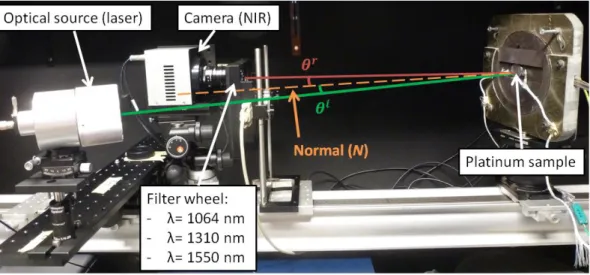
4.3. Diffusion function estimated by bichromatic thermoreflectometry on the platinum sample
The platinum sample studied before was heated at 530°C with the experimental set up of Fig. 6. Two geometrical settings were used. The first setting, named “symmetrical” (see Fig 6), is defined with the angle as: (𝜃𝑖, 𝜃𝑟, 𝜙) = (13°, 13°, 180°). Thus the maximum reflected flux is measured. The associated diffusion function is noted:
𝜂13,13. The second setting, named “asymmetrical”, is defined with the angle as: (𝜃𝑖, 𝜃𝑟, 𝜙) = (13°, 0°, 180°). The
associated diffusion function is noted: 𝜂0,13.
A bi-chromatic thermoreflectometry measurement is performed [3]. The radiance temperature and bidirectional reflectivity images are captured by a Xenics Xeva NIR camera with an InGaAs matrix detector (320x256 pix) sensible from 0.9 to 1.7 μm. The wavelength selection is done by three interferential filters in a filter wheel. Each filter has a bandwidth of 50 nm respectively centred at the wavelength: 1064, 1310 and 1550 nm. Three lasers with the same wavelength as the filters and with a bandwidth of 1 nm are coupled in optical fiber and connected to a projector. The size of the illuminated area is similar to the sample diameter (30 mm).
Fig. 6. Experimental apparatus with 𝜃𝑖= 𝜃𝑖= 13° and 𝜙 = 180°
For each setting, radiance temperatures field and bidirectional reflectivities field are measured at the three wavelengths of the filter wheel. A detailed description of the radiometric and reflectivity calibrations used can be found in [3].Then, the thermoreflectometric system is solved on each pixel at the three wavelength couples as follows:
{𝐿0(𝑇𝑅 𝑟(𝜆 1), 𝜆1) = 𝐿0(𝑇, 𝜆1) × (1 − 𝜌𝜆1 𝑖,𝑟𝜂𝑟,𝑖) 𝐿0(𝑇𝑅𝑟(𝜆2), 𝜆2) = 𝐿0(𝑇, 𝜆2) × (1 − 𝜌𝜆2 𝑖,𝑟𝜂𝑟,𝑖) (10)
Where 𝐿0(𝑇𝑅𝑟(𝜆1), 𝜆1) is the Planck function applied to the radiance temperature 𝑇𝑅𝑟 measured in the direction 𝑟 and at the
wavelength 𝜆1. The diffusion function 𝜂𝑟,𝑖 and the true temperature 𝑇 are the unknowns of this system.
10.21611/qirt.2018.123
The average of all diffusion functions computed for each wavelengths couple and settings are presented in the table 1. More details about the solving method can be found in [3].
Table 1. Averaged diffusion function and directional emissivity identified by thermoreflectometry Wavelength couple [nm] Diffusion function 𝜂13,13 [sr] Diffusion function 𝜂0,13 [sr] Directional
emissivity 𝜀13 emissivity 𝜀Directional 0
𝜆1𝜆2 (1064 , 1310) 0.1386 0.5245 0.36 , 0.32 0.36 , 0.32
𝜆1𝜆3 (1064 , 1550) 0.1362 0.5073 0.37 , 0.32 0.38 , 0.33
𝜆2𝜆3 (1310 , 1550) 0.1352 0.5007 0.33 , 0.33 0.34 , 0.33
As expected, because of its definition (see Eq. (2)), the diffusion function has a strong dependence with the geometrical setting. The diffusion function is nearly four times higher in the asymmetrical setting than in the symmetrical. Indeed, the higher values of bidirectional reflectivities are naturally measured with the symmetrical setting. As the sample was heated at the same temperature in both setting, all the changes of reflectivity are absorbed by the diffusion function in order to lead to a similar identified true temperature and associated emissivity. That is why the emissivities in the table 1 are consistent between the two settings.
Another remark is that the dispersion of the diffusion functions between all wavelength couples is low (2.5% relative difference for 𝜂13,13 and 4.5% for 𝜂0,13). A decreasing of the diffusion function with the increasing of the
wavelength couple is also observed in both settings. This could come from slight wave-optics effect which can affect the shape of the BRFD. Nevertheless this behaviour was not found in all the measurement. The diffusion function variations could be then explained by the measurement uncertainties.
In the next subsection, the diffusion function of the symmetrical setting will be compared to the theoretical curve of the diffusion function model (see Eq. (9)) as function of the standard deviation slope. The curve model of the asymmetric setting will be also presented with an illustration of its sensibility to the angular setting.
4.4. Analyse of the diffusion function and comparison with the experimental estimation
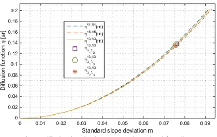
The objective is to study the shape of the diffusion function presented in Eq. (9) and depending only on the standard deviation of the slopes 𝑚 and the angular setting. The two angular settings used in 4.3 are reminded bellow:
- Symmetric setting noted 𝜂13,13 with (𝜃𝑖, 𝜃𝑟, 𝜙) = (13°, 13°, 180°)
- Asymmetric setting noted 𝜂0,13 with (𝜃𝑖, 𝜃𝑟, 𝜙) = (13°, 0°, 180°)
The diffusion function model and the experimental values identified by thermoreflectometry with a symmetrical setting are plotted on figure 6 with two near angular settings to evaluate the possible dispersion of the experimental setup.
Fig. 6. Diffusion function in a symmetric setting (𝜃𝑖= 𝜃𝑟= 13° ± 2°)
First, the evolution of the diffusion function model is monotonic and increasing with 𝑚. The diffusion function then grows with the spreading of the slope distribution of the surface. Second, the dispersion of the diffusion function value is low versus the dispersion of the configuration. The diffusion function model is not much affected by the change of the angle as long as the symmetry is preserved. Third, a single value of the roughness parameter 𝑚 with the experimental values of the diffusion function is estimated. The standard slope deviation value estimated is then between 0.0753 and 0.0762. These values can be compared to the measured values (subsection 4.1 m=0.085) and the estimated
14
thQuantitative InfraRed Thermography Conference, 25 – 29 June 2018, Berlin, Germany
8
value (subsection 4.2 m=0.0896). These three methods: roughness measurement, BRDF and thermoreflectometry experiments, provide consistent results between them and a low dispersion of the m identified.
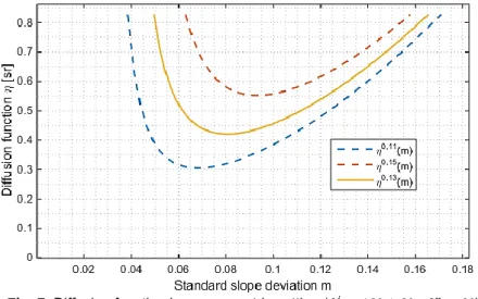
The asymmetric curves of the diffusion function model are presented on figure 7 with again two near angular settings.
Fig. 7. Diffusion function in a asymmetric setting (𝜃𝑖= 13° ± 2° ; 𝜃𝑟 = 0°)
First, the shape of the curves of the diffusion function is parabolic with a non-zero minimum. Second, the curve is very sensible to the angle set, especially for the low value of m. A small variation of the angle causes a strong variation of the diffusion factor. The estimation between the diffusion function and 𝑚 is then not as simple as in the symmetrical setting. Two different values of 𝑚 can give the same value of the diffusion function and reciprocally. Third, this angular sensibility of the diffusion function could be used to quantify the flatness defect of a surface with the assumption of a homogenous roughness. Also, the non-null minimum of the diffusion function can be exploited in the research of the solution of the thermoreflectometric system. This boundary can thus be interpreted with the value of the bidirectional reflectivity as a minimum reflectance or a maximum emissivity. Nevertheless this last remark should be taken precociously since this minimum strongly depends on the setting angle.
Finally, two behaviours of the diffusion function were observed depending on the choice of the angular setting. In the symmetrical case, a roughness parameter can be identified by the diffusion function and also the setting has a low dependence on the angle. In the asymmetric case, the parabolic shape and it high sensibility to the setting angle prevent all extrapolations of the standard slope deviations based on thermoreflectometric measurement. Despite that, this setting could be us to detect waviness defect or to improve the research of the thermoreflectometric system solution.
5. Conclusion
In the frame of the development of thermoreflectometry, the choice of the diffusion function regarding the materials studied is essential for the accuracy and validity of the method. In this article, a diffusion function, based on a physical model of BRDF, depending on a roughness parameter and the optical property of the material, was detailed. The model describes the case of rough metallic surface with a roughness size compatible with the geometric approximation. Then, with the appropriate angular setting and roughness, it can be showed that the diffusion function does not depend on the wavelength but only on the slope distribution of the surface.
Tests on a platinum sample show consistent results between the model and the experimental BRDF. The study of the diffusion function highlights two behaviours, depending on of the angular settings. In a symmetrical setting the identification by thermoreflectometry of the standard deviation of the slope is possible thanks to the shape of the function. In an asymmetric setting, the model becomes more sensible to the values of the setting angles and its shape prevents all roughness identification.
These results will have to be validated on others sample. Finally, some improvements on the model need to be included on the spectral dependence of the diffusion function. Research will be focused on wave-optic for the slightly rough materials and on volume scattering for dielectric materials as polymer or ceramic.
10.21611/qirt.2018.123
REFERENCES
[1] P. Herve, L. Viellard and A. Morel, « Radiométrie : L’ultraviolet (radiometry the ultraviolet) », Revue pratique de contrôle industriel, vol. 36, nᵒ 205, p. 60‑90, 1997.
[2] T. Duvaut. « Comparison between multiwavelength infrared and visible pyrometry: Application to metals ». Infrared Physics & Technology 51, no 4 (mars 2008): 292 99.
[3] T. Sentenac, R. Gilblas, D. Hernandez and Y. Le Maoult. « Bi-color near infrared thermoreflectometry: A method for true temperature field measurement», Review of Scientific Instruments, 83(12), 2012
[4] R. Gilblas, T. Sentenac, D. Hernandez and Y. Le Maoult. « Quantitative temperature field measurements on a non-gray multi-materials scene by thermoreflectometry », Infrared Physics & Technology, 66,2014, p. 70 77. [5] K. Tang, R. A. Dimenna and R. O. Buckius, « Regions of validity of the geometric optics approximation for
angular scattering from very rough surfaces », International Journal of Heat and Mass Transfer, vol. 40, no 1, p. 49-59, 1996.
[6] K.E. Torrance and E. M. Sparrow. « Theory for Off-Specular Reflection From Roughened Surfaces ». JOSA 57, no 9, 1967,1105 14.
[7] P. Beckmann et A. Spizzichino, The scattering of electromagnetic waves from rough surfaces. 1987. [8] R. L. Cook and K. E. Torrance, « A reflectance model for computer graphics », ACM SIGGRAPH Computer
Graphics, vol. 15, no 3, p. 307-316, 1981.
[9] A. D. Rakić, A. B. Djurišic, J. M. Elazar, and M. L. Majewski. Optical properties of metallic films for vertical-cavity optoelectronic devices, Appl. Opt. 37, 5271-5283 (1998)