HAL Id: hal-01271140
https://hal.archives-ouvertes.fr/hal-01271140
Submitted on 8 Feb 2016
HAL is a multi-disciplinary open access
archive for the deposit and dissemination of
sci-entific research documents, whether they are
pub-lished or not. The documents may come from
teaching and research institutions in France or
abroad, or from public or private research centers.
L’archive ouverte pluridisciplinaire HAL, est
destinée au dépôt et à la diffusion de documents
scientifiques de niveau recherche, publiés ou non,
émanant des établissements d’enseignement et de
recherche français ou étrangers, des laboratoires
publics ou privés.
Minimal Access Point Set in Urban Area Wifi Networks
Dareen Shehadeh, Nicolas Montavont, Tanguy Kerdoncuff, Alberto Blanc
To cite this version:
Dareen Shehadeh, Nicolas Montavont, Tanguy Kerdoncuff, Alberto Blanc. Minimal Access Point
Set in Urban Area Wifi Networks. WiOpt 2015 : 13th International Symposium on Modeling and
Optimization in Mobile, Ad Hoc and Wireless Networks, May 2015, Mumbai, India. �hal-01271140�
Minimal Access Point Set in Urban Area Wifi
Networks
Dareen Shehadeh, Nicolas Montavont, Tanguy Kerdoncuff, Alberto Blanc
Institut Mines Telecom / Telecom Bretagne, Irisa, Rennes, France {firstname.lastname}@telecom-bretagne.eu
Abstract—Faced by the large number of deployed Wifi Access Points (AP), many research efforts focus on energy savings in Wireless Local Networks. One of the most promising solutions for improving energy efficiency is the Sleep Mode approach, which is especially effective in dense deployments. It is based on switching off the APs while they are not in use, in order to avoid unnecessary energy consumption. In this paper we evaluate the poten-tial of switching off APs using real measurements taken in a dense urban area. We collected traces covering more than 20 hours, confirming the high density of currently deployed APs in such an environment. Based on these traces, we evaluate how many APs can be switched off while maintaining the same coverage. To this end, we propose two algorithms that select the minimum set of APs needed to provide full coverage. We compute sev-eral performance parameters, and evaluate the proposed algorithms in terms of the number of selected APs, and the coverage they provide. Our results show that between 4.25% and 10.91% of the detected APs are sufficient to provide the same coverage, depending on the data set, the mobile terminal and the AP selection algorithm.
I. INTRODUCTION
WiFi is probably the most popular short-range wire-less access technology with an exponential increase of Access Points (AP) deployments for the past few years [1]. They are being deployed in companies, schools, public and private areas; resulting in a high APs density and overlapping coverage areas. Usually all APs are switched on all the time, even when the number of users served by the wireless access network is very low, resulting in a high and partially wasteful energy consumption. Even though a single AP consumes only few watts, the total energy consumed could reach hundreds of watts in large deployments. For example, according to [2] the ADSL boxes (which are usually APs too) in France consume 5TWh per year. Tsui et al. [3] detected over 103000 APs in the city of Taipei through war-walking, while Achtzehn et al. [4] estimated the density of APs deployed in different cities in Germany to vary between 488 AP
per km2 in industrial areas, and 6103 AP per km2
in urban residential areas. Faced by AP proliferation and with the goal of reducing the energy consumption, recent research efforts have proposed algorithms to This work has received a French government support granted to the CominLabs excellence laboratory and managed by the National Research Agency in the “Investing for the Future” program under reference ANR-10-LABX-07-01
dynamically switch on and off a set of APs depending on the traffic load.
In continuity with these efforts, we study in this paper the Wifi AP deployment in an urban environ-ment and evaluate the AP redundancy in providing network coverage. We provide a methodology and a set of tools to measure this density. Using the Android application Wi2Me to performs network scanning, we gather real data about APs through war-walking in the centre of Rennes - France. After processing these data with various filters, we apply two different selection algorithms to select a minimal set of APs that are enough to provide the same coverage, assuming that the non-selected APs could be switched off.
The rest of the paper is organized as follows: Sec-tion II provides an overview of related works, mainly on the sleeping approaches in WLANs. Section III gives an overview of the platform we used and describes the methodology we followed. Section IV presents the different processes and filters applied on the raw data before applying the two proposed algorithms for AP se-lection described in Section V. In Section VI we present and discuss the results of this study. Finally, conclusions and future work are presented in Section VII.
II. RELATED WORK
Several papers [5]–[8] have proposed strategies to reduce energy consumption in dense WLANs by turn-ing APs on and off, exploitturn-ing overlappturn-ing coverage areas. Some authors [9], [10] propose to use an addi-tional low power radio interface to communicate control information among APs when their Wifi interfaces are switched off.
Jardosh et al. [5] propose a “resource-on-demand” (RoD) strategy to dynamically switch on and off APs in dense WLAN. They group nearby APs in clusters, where one single leading AP from each group is sufficient to provide basic coverage to users in the cluster. Only this AP is kept on while other APs in the cluster are switched off. When the number of users increases, additional APs can be switched on to cope with the increased demand. Energy saving is estimated to be up to 80% in really dense environment, while it is about 20% to 50% in less dense WLANs. Two improvements were suggested in [6]. The first is to take into account the number and signal strength of
received beacons to identify the neighboring APs when forming a cluster. The second improvement was to use the channel utilization to estimate the user demand. Thanks to an experimental setup, the authors show that it is possible to achieve energy savings of up to 53% when traffic is low and 16% when traffic demand is high.
In a similar setting, Marsan et al. [7], propose two policies to turn on and off certain APs and a corre-sponding analytical model. The first policy depends on the number of users in a cluster, while the second is based on the amount of traffic that is handled by the cluster. Through simulations, they evaluate the perfor-mance of these two policies under different conditions of traffic load during 1-day period. Their results show that 40% of the energy can be saved.
Ganji et al. [8], [11] address enterprise WLANs, proposing to switch off APs when traffic is low, keeping only a few APs on to maintain coverage and to detect user presence. When user connections are detected, the appropriate APs are switched on in order to provide the required service. The authors evaluate the performance of the proposed strategy through Matlab simulations for both IEEE 802.11g and IEEE 802.11b networks, show-ing that achievable power savshow-ings in dense WLANs are in the range of 98% of total consumed power, where the number of APs needed to provide coverage for the considered area is about 1% of the total number of APs. A different approach, using an additional “low-power-wake-up” radio link module is presented in [9]. In this approach only the Wifi radio part which con-sumes most of the energy supplied to the AP is turned off. An additional low power radio module is added to both the AP and the terminal to exchange out-of-band control information when the wifi radio interface is turned off. Users’ requests for a connection are handled by this low-power radio link that is always active, maintaining connectivity and waking up the AP when necessary. In order to evaluate their proposal they set-up a prototype and measure the energy consumption gain and wake-up delay. They show that, while the the-oretical maximum reduction in the power consumption is 28.57%, the actual total power saved is 22.9% and the average wake-up delay is around 10 seconds.
Similarly, Kumazoe et al. [10] propose the use of additional wake-up receivers attached to APs. An AP automatically switches off when it detects no activity in the network for a predefined period of time and it hands-off its users to another active AP, selected based on the utilization of the active APs. In order to prevent excessive aggregations of users on an AP, a control mechanism is applied, which requires a periodical ex-change of channel utilization information among the APs. Through simulation, the authors show that their solution can reduce power consumption by 40%.
Lorincz et al. [12] tackle the problem of finding the optimum network configuration in terms of power consumption while guaranteeing coverage and enough capacity to serve active users in WLANs. They use an
integer linear program (ILP) to minimize the number of active APs under coverage constraints. This model assumes that it is possible to know the location of users, so that coverage can be optimized for the actual traffic demand. Numerical results show that the proposed approach is actually able to modulate instantaneous power consumption of the network based on the traffic needs achieving up to 63% in energy savings.
Strikingly, these studies give significantly different energy savings, from 16% to 98%. This can be ex-plained by the different scenarios considered in each study. Some studies are based on simulations, others on real measurements, but the most important factor is whether they consider a dense environment or not. Obviously there is a bigger opportunity for energy ef-ficiency in over-dimensioned networks, specially when traffic is low. In this paper we try to assess the effec-tiveness of turning off certain APs in a real setting, namely a dense urban environment. Valadon et al. [13] use a similar methodology of war-walking to evaluate the density of APs in two districts in Paris. According to their results, there are between 3107 and 5090 AP per
km2, so that most of them have overlapping coverage
areas. Such a high AP density should indeed be enough to allow for significant energy efficiency by turning some of them off. We want to estimate the minimum number of APs needed to provide the full coverage of a certain path. Imitating the behaviour of a mobile user, we collect information about the available APs by walking in a dense urban area and we use these measurements to estimate how many APs we could turn off while still offering full coverage.
III. DATACOLLECTION
Our goal is to characterize and analyze real urban environment in terms of number of APs deployed, their density and their coverage areas. We want to evaluate the AP redundancy and identify how much the AP density can be reduced while still providing connectivity for mobile users. Fig. 1 summarizes the different steps we took to compute the minimal AP set. First, we walked for more than 20 hours in the center of Rennes (France) carrying smartphones run-ning the Wi2Me application [14] (“war-walking”). This application scans periodically all the WiFi channels and logs all the available APs, generating a set of Wi2Me Traces, containing the time, the GPS location and other information about the discovered AP. We then process one or more of these traces to produce a Coverage Matrix, summarizing the APs observed. The Coverage
Matrixis converted to an Input Matrix, which is finally
used as the input of different algorithms that select the Minimal AP Set, that is a significantly smaller set of APs providing almost the same coverage as all the APs detected.
Wi2Me is an Android-based application that per-forms network discovery through scanning, automatic connection and data traffic generation using the 802.11 and 3G interfaces of Android smartphones. The mobile
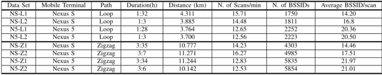
Data Set Mobile Terminal Path Duration(h) Distance (km) N. of Scans/min N. of BSSIDs Average BSSID/scan NS-L1 Nexus S Loop 1:32 4.311 15.71 1750 14.20 NS-L2 Nexus S Loop 1:3 3.885 14.48 1811 16.8 N5-L1 Nexus 5 Loop 1:28 3.764 12.65 2252 20.36 N5-L2 Nexus 5 Loop 1:3 3.700 12.56 2223 20.50 NS-Z1 Nexus S Zigzag 3:35 10.777 14.23 4303 14.46 NS-Z2 Nexus S Zigzag 3:7 11.271 16.27 4985 17.51 N5-Z1 Nexus 5 Zigzag 3:34 11.244 12.83 5835 21.97 N5-Z2 Nexus 5 Zigzag 3:6 10.142 12.53 5854 21.01
TABLE I: Traces and Measurements.
Wi2Me Trace Coverage
Matrix Input Matrix Minimum AP Set Extract Data P r ocess D ata ApplyAP selection-Algorithm
Fig. 1: Methodology diagram
terminal performs periodic scanning in all channels. In each scanning cycle, the mobile terminal starts from channel number 1, sends two probe requests, waits for responses from APs, then moves on to the next channel and repeats the process until reaching channel number 13. The time for which a mobile terminal waits on each channel is device dependent, and for the devices we used in our measurements, this time was between 80 ms and 130 ms per channel resulting in about 1.70 s for all the channels. Having finished a scanning process, the mobile terminal waits for some time before re-initiating a new one. This waiting time is preconfigured in the devices and it was set to 3 s. This value was chosen based on previous studies in order to avoid receiving responses from a previous scanning cycle during the current one. The mobile terminals were scanning during the entire measurement campaign, i.e., they never tried to associate with an AP.
During each scanning phase, information about available APs are collected and stored as a scanning
event in a database called Wi2me Trace. A scanning
event includes information about each detected AP such as BSSID, SSID, channel number, signal level, supported security protocols, link data-rate, GPS coor-dinates of the mobile terminal and a timestamp.
We chose two different paths in downtown Rennes. The first path is a 3.7 km Loop on major streets (see Fig. 2a). The second path is a 10 km Zigzag path (see Fig. 2b). In the first path, we wanted to avoid as much as possible detecting the same AP twice, hence we followed a roughly rectangular path. On the contrary, in the Zigzag path we took a winding route through smaller streets, and thus we were able to detect the same APs from different places. The idea behind this was to get two different sets of data representing two radically different real life itineraries of a mobile user and then apply our AP selection algorithms to both cases.
We covered each path four times, carrying two
ter-(a) Map of the Loop Trace (b) Map of Zigzag Trace
Fig. 2: The wardriving in Down town Rennes -France
minals running Wi2Me. The first terminal is a Samsung Nexus S to which we attached an external antenna of 3 dBi gain. The second terminal is a Samsung Nexus 5. The war-walking was done at an almost constant speed of 1 m/s.
Table I contains some of the results that we ob-tained. As we compute the total distance covered based on the GPS coordinates, results show different lengths for each traces due to the cumulative GPS errors. The results also show different numbers of scans and discovered APs for each path and trace. This is due, on the one hand, to the random variability of the link quality between the APs and the terminals; and on the other hand, to the device characteristics and the actual scanning duration. In particular, we notice that the Nexus 5 has a better wireless performance than the Nexus S for the number of APs detected and the average number of APs per scan. The results also show that around 2000 different BSSIDs were discovered in the Loop Traces, and up to 5854 APs in the Zigzag path. The average scanning rate is about 15 scans per minute for Nexus S and the average number of detected APs per scan is 14, while the scanning rate in the Nexus 5 is about 12 scans per minute with an average number of APs detected per scan of 20. These results are consistent with our observations in previous studies [15] and with the results of [3].
IV. DATAPROCESSING
In this section we explain how we processed the Wi2Me Traces to obtained the raw Coverage Matrix, which is then transformed into the Input Matrix, as illustrated in Fig. 1.
Fig. 3: Coverage Matrix
A. The Coverage Matrix
In order to represent the coverage of each AP, we build a Coverage Matrix, where each line corresponds to a scanning event and each column to an AP. If a given AP was detected during a scanning event, the corresponding element in the matrix is one, and zero otherwise. Thus the ones in a given line represent all the APs detected in the corresponding scanning event (i.e., AP from which the mobile terminal received either a probe response or a beacon). The ones in a given column indicate all the scanning events where a given AP was discovered. Thus the coverage of an AP can be defined as the set of ones in the corresponding column. Fig. 3 shows an example of the Coverage Matrix. We call Continuous Coverage of an AP, the parts of the column in the Coverage Matrix where there are successive ones and no zeros in between. While Total
Coverage of an AP is the total of all scanning events
where it was discovered, i.e., the set of all ones in the column representing the AP in the Coverage Matrix.
In the rest of the section we describe how the data of the Coverage Matrix is analysed and processed in order to build the Input Matrix, used by the selection algorithms.
B. Detecting Physical APs
It is often the case that a large number of APs announce multiple networks. Each of these networks is assigned a different SSID and BSSID. Usually, these BSSIDs are all derived from the MAC address of the AP. Analysing the Wi2Me Traces, we noticed that some co-located BSSIDs have MAC addresses very similar to each other and they only differ in the value of the last byte or first byte (depending on the operator). Since we are only interested in the coverage that a physical AP provides, and not in the different networks it advertises, we group these BSSIDs and treat them as one physical AP in the Input Matrix. This is done by combining all the columns of similar BSSIDs in one
100 101 102 103 104
Size of Gaps (Logarithmic scale) 0.0 0.2 0.4 0.6 0.8 1.0 CDF fo r t he si ze of G ap s
Fig. 4: AP coverage gap size distribution
column. By doing so we obtain a number of physical APs corresponding to roughly 70% of the total number of BSSIDs for each trace.
C. Coverage Gaps
Especially in the Loop path, we would expect a continuous coverage of each AP. Recall that each row in the matrix corresponds to a scanning event, which in turn corresponds to a given location and timestamp. Therefore we would expect the columns of the Cover-age Matrix to have long runs of consecutive ones, as each column corresponds to a single AP. But this is not the case for all the APs. Analyzing the Coverage Matrix, we find gaps of different sizes in the coverage of APs, i.e., we find zeros between runs of ones, as highlighted in Fig. 3. Fig. 4 shows the cumulative distribution of the size of the gaps for one of the Loop traces. It shows that the size of the gaps varies from 0 (corresponding to no gap in the coverage) to 3000. About 80% of them are of a size smaller than 10. Such a small size for the vast majority of the gaps seems to indicate that they were caused by the terminal not being able to exchange messages with the AP for a few scanning events, for instance because of random channel fluctuation. This is consistent with what we have observed in a previous study [15]: occasionally probe requests, probe responses or beacon messages can be lost during the scanning procedure, even if the terminal is within the coverage area of the AP. Applying the Selection Algorithm on the raw data, including these spurious coverage gaps, would lead to an overly pessimistic coverage set, as the algorithm would need to include in the minimal AP set a number of APs to cover these spurious gaps. This is reinforced by the fact that these data belong to a single trace. As we discuss in Section IV-E, we addressed this problem by merging multiple traces for the same path: if a certain point is indeed within the coverage area of an AP we expect to be able to detect at least once during our measurements. Some of the gaps could indeed correspond to actual
coverage gaps, for instance because of an obstacle (building, tree, etc.). In the case of the Zigzag path, this could also be caused by the user starting to move away from the AP only to move closer shortly thereafter because of the shape of the path. The Loop path should not have such a problem as it is a straight line most except for the four turns, as mentioned in Section III. These gaps are handled by the Selection Algorithm that is going to select another AP to compensate for the absence of coverage (see in Section V).
Another possible explanation for some of the gaps is the re-use of MAC address, i.e., two (or more) different physical APs, located in different places, using the same BSSID. This is most likely the case for the larger gaps. We have confirmed this by plotting the positions of some of these BSSIDs on a map, which showed that the positions are grouped in two or more different locations and could not possibly belong to the same AP. The following section addresses this problem in more details.
D. MAC Address Re-use
In order to separate the APs that share the same MAC address, we developed a technique depending on the SSID information available in the Wi2Me Traces. As it is known, an AP can advertise several SSIDs each with a different MAC address. Many of the announced SSIDs of an AP are commonly used among different APs of the same operator. Only the SSID of the private network that belongs to the owner of the AP is different. Thus it is possible to separate the different APs that are using the same MAC address depending on the SSIDs of the private network. First, for each column in the Coverage Matrix we filter the SSIDs depending on the private ones. Then we separate them creating a new column for each private SSID. Applying this technique, we find that 1% of the APs share the same MAC Address.
The drawback of this method is that we do not always receive all the SSIDs broadcasted by an AP, and thus we might miss the private network SSID (failing to detect MAC address re-use). To address this problem, we covered the same paths using a Dell Latitude E4300 laptop running Linux. The advantage of these traces is that they contain the uptime of the AP included in the TSF field used for clock synchronisation and included in the beacons and probe responses. We compared the uptime value of the AP to the clock of the laptop, and we calculated the offset, i.e., the difference between these two values. As long as this offset is below a certain threshold, we conclude that the message was sent by the same AP. On the contrary, if the offset is above the threshold, we conclude that two different APs are using the same MAC address.
Fig. 5 shows the percentage of MAC addresses that are never reused (top curve) and those that are reused at least once (bottom curve), as a function of the threshold. It is easy to see that both curves stabilize quickly after roughly 75 ms. Using a 100 ms threshold for the Loop
traces, we find that 2.6% of the detected APs reuse MAC addresses.
Comparing these two techniques, we found that the SSID method detected only 41.22% of the MAC address re-use detected by the time offset method. We examine the APs undetected by the SSID method to see if they introduce any anomaly when applying the selection algorithms. We found that these undetected MAC reuse cases belong to APs with minimal coverage. This makes sense because APs coverage correlates to detectability of the private SSID.
For these reasons, and because of the small subset of APs it concerns (around 2% of APs re-use MAC addresses), we consider that the SSID technique is suffi-cient to provide reliable android data to our algorithms. E. Merging Traces
As mentioned above, some of the AP coverage gaps, detected in a single trace, can be caused by random fluctuations in the radio link quality. It is possible to address this problem by combining different traces covering the same path. This is possible thanks to the GPS coordinates associated to each scanning event. As different traces never have exactly the same coordinates, we operated as follows: using data from Open Street Map, we divided each path into 1 m segments, then the location of each scanning event is projected orthogo-nally to the closest street in the path. In the case of merged traces, the rows of the Input Matrix correspond to the 1 m segments and not to the scanning events. If the AP is detected in two successive scannings in the Coverage Matrix, we consider that it is present in all the segments between the projection points of these two scannings in the Input Matrix and thus the lines of the corresponding column are filled with ones. It is worth underlining that these ones are added only if the AP was detected in two consecutive scanning events in the Coverage Matrix; in other words, all the coverage gaps present in the Coverage Matrix are preserved.
Once we have converted the Coverage Matrices to Input Matrices with rows corresponding to the 1-meter segments, we can combine them using the following two steps, the first determines the column of the merged matrix and the second determines the one and the zeros:
1) Identifying APs: Some APs are present in only
one of the traces, typically because their messages were received with low power. As such, they are poor candidates for the minimal AP set. Therefore, in the merged matrix, we keep only the APs that have been detected in each trace. This corresponds to a logical AND between the columns of the Input Matrices of each trace.
2) Filling the Input Matrix: We use logical OR
between the rows of the Input Matrices. Thus an AP is considered present at a given geographical position if there was at least a one at this position in any of the matrices being merged. As we have previously mentioned, this is done because, due to the random
fluctuations of the radio channel, it can happen that an AP was not detected at a given point even though that point is well within the coverage area of the AP.
V. AP SELECTIONALGORITHMS
As we expected and as it has been shown by several studies [3], [4], the Coverage Matrices of the two paths show that there is a large number of APs with overlapping coverage. Finding the smallest set of APs to cover the whole path is an instance of the set cover problem, one of the classical examples of NP-Complete problems. We have used two algorithms to compute a smaller covering set.
The first one is the well known greedy algorithm for the set cover problem [16]. As this algorithm tries to minimize the number of APs by first selecting those with the largest coverage, it then uses a certain number of APs to cover the gaps between APs with larger coverage. In the context of a WLAN, this is not necessarily the ideal solution as the APs used to fill these gaps can have a fairly small coverage area, causing mobile users to have more handovers and to be associated for a short period of time to these APs.To address this problem, we propose another simple greedy algorithm called Greedy Continuous (GC), whose main idea is to start at some point on the path, select the AP with the longest coverage from the current position, then move to the end of the coverage area of the selected AP and repeat the process until the whole path has been covered.
A. The Greedy Algorithm
In the usual formulation of the set cover problem, we are given a set of sets (S), whose union is called the universe; the goal is to find the smallest subset of S. In our setting, the union of the lines of the Input Matrix is the universe and each column of the matrix is an element of S. The algorithm works as follows:
Step 1: Calculate the total coverage value for the APs, i.e., the sum of all the ones in the corresponding column of the Input Matrix.
Step 2: Select the AP with the largest total coverage value and add it to the Minimum APs Set.
Step 3: Delete the lines where there is a one in the column of the selected AP from the Input Matrix.
Step 4: Delete the column of the selected AP from the Input Matrix.
Step 5: Go to Step 1 and repeat until all the lines are deleted.
B. The Greedy Continuous Algorithm
This algorithm uses a local optimization criteria that consists of selecting the AP with the longest continuous coverage for the next part of the path, and it works as follows:
Step 1: Starting from the beginning of the path, i.e., the first line of the Input Matrix, identify the available APs (the columns where there are ones in this line).
Step 2: Calculate for each of these APs the continu-ous coverage (sum of successive ones starting from the current position until the first zero).
Step 3: Choose the AP with the longest continuous coverage and add it to the Minimum APs Set.
Step 4: Go to the last line of the continuous coverage of the selected AP.
Step 5: Repeat steps 2 to 4 until the end of the matrix i.e end of the path.
VI. RESULTS
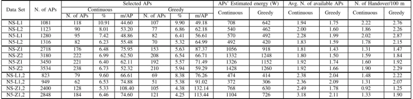
We applied the two algorithms presented in the previous section to the dataset presented in Section III. For each Trace, we build an Input Matrix by grouping BSSIDs, identifying MAC address re-use, and correct-ing the GPS coordinates as explained in Section IV. We also merged the traces as discussed in Section IV-E and applied the algorithms to the resulting Input Matrices. Table II summarizes some of the results for each algorithm, including the number of selected APs and the number of handovers, i.e., the number of handover that a user would have to make if she followed the same path and only the selected APs were active.
A. AP Redundancy
As mentioned earlier, our main objective in this study is to evaluate the redundancy of APs in a dense urban deployment, and see by how much the number of operating AP can be reduced, while maintaining the same coverage. The results in Table II show that, on average, around 6.5% of the detected APs are sufficient to provide full coverage of the path. This percentage varies from 4.25% to 10.91% depending on the dataset, the phone, and the AP selection algorithm. In other words, we can maintain the coverage of a path while switching off at least 89% of the existing APs. This means that the potential of energy saving obtained by switching off the non selected APs is about 89% too. We estimated the energy consumed by the selected APs using the results of [17], which reported that the average consumption of a single AP is about 6 W. Results show that the selected APs consume around 540 W in average for the Loop path and 1215 W for the Zigzag path. This reflects a significant reduction in energy consumption when compared to the initial estimated consumption of 7200 W and 19 323 W for the two paths respectively.
Results also show that the minimal AP set offers a good overlapping. The number of APs seen at any position of the path varies between 1 and 6, with a mean of approximately 2, and an overlapping of two or more APs along more than 60% of the path. Compared to the initial situation where we had an average of 17 APs present at each position of the path (see Table I), this represents a large reduction in overlapping. The overlapping in the minimal set is useful to insure smoother handovers.
Data Set N. of APs
Selected APs APs’ Estimated energy (W) Avg. N. of available APs N. of Handover/100 m
Continuous Greedy
Continuous Greedy Continuous Greedy Continuous Greedy
N. of APs % m/AP N. of APs % m/AP
NS-L1 1081 118 10.91 44.60 107 9.90 49.18 708 642 1.94 1.75 2.22 2.76 NS-L2 1123 90 8.01 53.20 77 6.86 62.18 540 462 2.00 1.60 1.86 2.26 N5-L1 1280 95 7.42 48.86 82 6.41 56.61 570 492 2.28 1.99 2.02 2.87 N5-L2 1316 82 6.23 55.48 70 5.32 64.99 492 420 1.83 1.59 1.78 2.15 NS-Z1 2718 176 6.48 75.95 153 5.63 87.37 1056 918 1.81 1.43 1.31 1.47 NS-Z2 3180 222 6.99 62.50 208 6.54 66.71 1332 1248 1.80 1.50 1.59 1.84 N5-Z1 3450 221 6.40 62.11 192 5.57 71.49 1326 1152 1.92 1.74 1.60 1.92 N5-Z2 3534 238 6.73 52.32 210 5.94 59.29 1428 1260 1.92 1.66 1.90 2.29 NS-L1,2 823 79 9.60 66.61 69 8.38 76.26 474 414 2.38 2.04 1.48 2.22 N5-L1,2 949 62 6.53 74.88 51 5.38 91.02 372 306 2.36 2.09 1.31 2.07 NS-Z1,2 2400 128 5.33 108.40 105 4.38 132.14 768 630 2.49 1.78 0.92 1.25 N5-Z1,2 2848 184 6.46 74.60 121 4.25 113.44 1104 726 3.18 2.11 1.33 1.90
TABLE II: Results of applying the algorithms
Separated AP s (% ) 0 20 40 80 60 100 Offset threshold (ms) Reused mac addresses Never reused mac addresses
Fig. 5: AP seperation depending on the offset threshold
0 2 4 6 8 10 12
AP Cont ribut ion (%) 0.0 0.2 0.4 0.6 0.8 1.0 C D F GC Greedy
0 50 AP Cont ribut ion (m )100 150 200 250
Fig. 6: CDF of APs Contribution to Coverage Selected APs (%) Re m ai ni ng C ov er ag e (% )
Fig. 7: Trade off between N. of selected APs and Coverage
B. Marginal AP Coverage Contribution
In the minimal AP set, not all APs contribute evenly to the path coverage. This is particularly true for the results of the greedy algorithm since some APs are only selected to cover a small gap and thus provides minimal additional coverage. Fig. 6 illustrates this, by showing the percentage of marginal contribution to the coverage of each AP (i.e., the additional (marginal) coverage contributed by each AP and not already covered by the previously selected APs). About 75% of the selected APs contribute to less than 2% of the total coverage of a path each. It also shows that for the greedy algorithm only 5% of the selected APs contribute to more than 6% of the coverage each, while for the GC algorithm the APs contribute more evenly to coverage.
When measuring the APs’ marginal contribution in meters (shown on top of the figure), one can notice that, for both algorithms, around 75% of the selected APs cover less than 40 m each. Only 5% of the APs cover more than 140 m each for the Greedy Algorithm, while this is not the case for the Continuous Algorithm. Fig. 7 shows the remaining coverage of a path when successively eliminating low coverage APs out of the minimal AP set. Consistently with the above results, this figure shows that we can maintain about 98% of the coverage even when eliminating 40% and 22% out of the selected APs for the greedy algorithm and the GC algorithm respectively.
C. Comparing the two Algorithms
The results show that, for any trace, the number of APs selected by the greedy algorithm is smaller than the number of APs selected by the GC algorithm. These results are consistent with the APs’ selection criteria used by each algorithm. The greedy algorithm selects AP with the large coverage areas first, so that it needs fewer APs to cover a path compared to the GC algorithm.
But if we look at the number of handovers required by a potential user that would move along this path using this minimal AP set, we see that the GC algorithm requires fewer handovers. This is because the greedy algorithm selects APs based only on the size of the coverage area and not the location of each AP, while the GC algorithm takes location into account. The AP coverage overlap provided by the two algorithms is similar (almost equivalent) with the GC algorithm being slightly better since it selects more APs. To summarise, the greedy algorithm is more efficient in terms of energy consumption since it selects fewer APs, while the GC algorithm provides better overal coverage (fewer handover and bigger overlap).
D. Merged Traces
Applying the merging technique, as described in Section IV-E, decreases the number of APs in the Input Matrix between 20% and 30%. This is because the Input Matrix contains only the APs that have been detected in all the traces. Recall that this is to eliminate APs that
have been usually detected in only one trace and with a low signal strength, making them bad candidates for the minimal set. Therefore such reduction in the number of APs should not affect the minimal set.
When applying the two algorithms on the merged traces, we find that the number of APs in the minimal set has decreased for both algorithms between 25% and 40%. This is a direct result of the second step of the merging technique that handles the cases where a mobile station misses an available AP due to low channel quality in one trace by finding a match in the other trace. Thus it tends to decrease the size of the gaps and increases the continuity of coverage of the APs (selected in the first step) by accepting that the AP be present in one of the traces. Consequently, this improves the performance of the two algorithms in terms of the number of required handovers and the number of the available APs present at each position by 10% to 30%.
VII. CONCLUSION
In this paper, we addressed the feasibility of re-ducing the number of active APs in an urban setting. We presented two algorithms to compute the minimal AP set and compared their performance using traces collected in the center of Rennes (France). The results show that it is possible to use only around 6.5% of the existing APs in order to provide the same coverage. The exact number of the selected APs depends on the dataset, the algorithm used, and the platform that is used to perform the measurements. Results vary from around 4.25% to 10.91%. Thus the potential of energy saving obtained by switching off the non selected APs could reach 95%. Results also show that the selected AP set provides an overlapping of a minimum of two APs along more than 60% of the path. The greedy algorithm is more efficient in terms of energy consumption since it selects fewer APs, while the GC algorithm provides better coverage since it requires fewer handovers.
As mentioned earlier, our algorithms only guarantee that users in a path are covered by at least one AP. Further investigations are required to evaluate how many users the minimal AP set can support, the traffic rate it can provide for them, and the tradeoff between the number of active APs and the resulting QoS. An-other possibility is to enhance the proposed algorithms in order to take into account constraints such as the minimum average APs present at each position and the maximum number of handovers allowed. Finally, it could also be possible to investigate how to assign the selected APs to the different Wifi channel in order to minimize the interference among them.
REFERENCES
[1] “Dartmouth collegewlan, http://crawdad.cs.dartmouth.edu.”
[2] P. OLIVIER, “Les box adsl vont gaspiller 3 twh en
2012,
http://www.greenit.fr/article/energie/les-box-adsl-vont-gaspiller-3-twh-en-2012-3516.”
[3] A. W. Tsui, W.-C. Lin, W.-J. Chen, P. Huang, and H.-H.
Chu, “Accuracy Performance Analysis between War Driving and War Walking in Metropolitan Wi-Fi Localization,” IEEE Transactions on Mobile Computing, vol. 9, no. 11, pp. 1551– 1562, Nov. 2010.
[4] A. Achtzehn, L. Simic, P. Gronerth, and P. Mahonen, “Survey
of ieee 802.11 wi-fi deployments for deriving the spatial structure of opportunistic networks,” in Personal Indoor and Mobile Radio Communications (PIMRC), 2013 IEEE 24th
International Symposium on. IEEE, 2013, pp. 2627–2632.
[5] A. P. Jardosh, G. Iannaccone, K. Papagiannaki, and B.
Vin-nakota, “Towards an Energy-Star WLAN Infrastructure,” Eighth IEEE Workshop on Mobile Computing Systems and Applications, pp. 85–90, Mar. 2007.
[6] A. P. Jardosh, K. Papagiannaki, E. M. Belding, K. C. Almeroth,
G. Iannaccone, and B. Vinnakota, “Green WLANs: On-Demand WLAN Infrastructures,” Mobile Networks and Appli-cations, vol. 14, no. 6, pp. 798–814, Dec. 2008.
[7] M. A. Marsan, D. Elettronica, L. Chiaraviglio, and D. Ciullo,
“A simple analytical model for the energy-efficient activation of access points in dense wlans,” 1st International Conference on Energy-Efficient Computing and Networking, pp. 159–168, 2010.
[8] F. Ganji, L. Budzisz, and A. Wolisz, “Assessment of the Power
Saving Potential in Dense Enterprise WLANs,” 2013 IEEE 24th International Symposium on Personal Indoor and Mobile Radio Communications (PIMRC), pp. 2835–2840, 2013.
[9] I. Haratcherev, M. Fiorito, and C. Balageas, “Low-power sleep
mode and out-of-band wake-up for indoor Access Points,” GLOBECOM Workshops, 2009.
[10] K. Kumazoe, D. Nobayashi, Y. Fukuda, T. Ikenaga, and
K. Abe, “Multiple Station Aggregation Procedure for Radio-On-Demand WLANs,” 2012 Seventh International Conference on Broadband, Wireless Computing, Communication and Ap-plications, pp. 156–161, Nov. 2012.
[11] F. Ganji, L. Budzisz, and A. Wolisz, “Telecommunication
networks group assessment of the power saving potential in dense enterprise wlans,” 2013.
[12] J. Lorincz, A. Capone, and M. Bogarelli, “Energy savings
in wireless access networks through optimized network man-agement,” IEEE 5th International Symposium on Wireless Pervasive Computing 2010, pp. 449–454, 2010.
[13] G. Valadon, F. L. Goff, and C. Berger, “A Practical
Character-ization of 802.11 Access Points in Paris,” 2009 Fifth Advanced International Conference on Telecommunications, pp. 220– 225, 2009.
[14] G. Castignani, A. M. Lampropulos, A. Blanc, and N.
Mon-tavont, “Wi2Me: A Mobile Sensing Platform for Wireless Heterogeneous Networks,” in ICDCS 2012: IEEE International Workshop on Sensing, Networking, and Computing with Smart-phones, 2012.
[15] L. Molina, N. Montavont, G. Castignani, and A. Blanc, “Access
point discovery in 802 . 11 networks,” Wireless Days, 2014.
[16] T. H. Cormen, C. E. Leiserson, R. L. Rivest, and C. Stein,
Introduction to Algorithms, Third Edition, 3rd ed. The MIT
Press, 2009.
[17] K. Gomez, R. Riggio, T. Rasheed, and F. Granelli, “Analysing
the energy consumption behaviour of WiFi networks,” 2011 IEEE Online Conf. on Green Communications, pp. 98–104,