Prioritising individual water mains for renewal

Publisher’s version / Version de l'éditeur:

Vous avez des questions? Nous pouvons vous aider. Pour communiquer directement avec un auteur, consultez la

première page de la revue dans laquelle son article a été publié afin de trouver ses coordonnées. Si vous n’arrivez pas à les repérer, communiquez avec nous à PublicationsArchive-ArchivesPublications@nrc-cnrc.gc.ca.

Questions? Contact the NRC Publications Archive team at

PublicationsArchive-ArchivesPublications@nrc-cnrc.gc.ca. If you wish to email the authors directly, please see the first page of the publication for their contact information.

https://publications-cnrc.canada.ca/fra/droits

L’accès à ce site Web et l’utilisation de son contenu sont assujettis aux conditions présentées dans le site LISEZ CES CONDITIONS ATTENTIVEMENT AVANT D’UTILISER CE SITE WEB.

ASCE/EWRI World Environmental and Water Resources Congress 2008 [Proceedings], pp. 1-10, 2008-05-12

READ THESE TERMS AND CONDITIONS CAREFULLY BEFORE USING THIS WEBSITE. https://nrc-publications.canada.ca/eng/copyright

NRC Publications Archive Record / Notice des Archives des publications du CNRC :

https://nrc-publications.canada.ca/eng/view/object/?id=510fc830-b43b-40d8-95d6-14b94ab8677e https://publications-cnrc.canada.ca/fra/voir/objet/?id=510fc830-b43b-40d8-95d6-14b94ab8677e

NRC Publications Archive

Archives des publications du CNRC

This publication could be one of several versions: author’s original, accepted manuscript or the publisher’s version. / La version de cette publication peut être l’une des suivantes : la version prépublication de l’auteur, la version acceptée du manuscrit ou la version de l’éditeur.

Access and use of this website and the material on it are subject to the Terms and Conditions set forth at Prioritising individual water mains for renewal

http://irc.nrc-cnrc.gc.ca

P r i o r i t i s i n g i n d i v i d u a l w a t e r m a i n s f o r

r e n e w a l

N R C C - 5 0 4 5 0

K l e i n e r , Y . ; R a j a n i , B .

A version of this document is published in / Une version de ce document se trouve dans: ASCE/EWRI World Environmental and Water Resources Congress 2008, Honolulu, Hawaii, May 12-16, 2008, pp. 1-10

The material in this document is covered by the provisions of the Copyright Act, by Canadian laws, policies, regulations and international agreements. Such provisions serve to identify the information source and, in specific instances, to prohibit reproduction of materials without written permission. For more information visit http://laws.justice.gc.ca/en/showtdm/cs/C-42

Les renseignements dans ce document sont protégés par la Loi sur le droit d'auteur, par les lois, les politiques et les règlements du Canada et des accords internationaux. Ces dispositions permettent d'identifier la source de l'information et, dans certains cas, d'interdire la copie de

Prioritising individual water mains for renewal

Abstract

The statistical analysis of historical breakage patterns of water mains is a cost effective approach to discern their deterioration, where physical mechanisms that lead to their deterioration are often very complex and not well understood. Furthermore, data required to model these physical mechanisms are rarely available and prohibitively costly to acquire.

Several models exist in the literature, which use various statistical methods to analyse patterns of pipe breakage histories. Some of these models were designed to address relatively large groups of pipes, which are presumed to be homogeneous with respect to their deterioration patterns, while others address individual water mains. However, predicting a breakage pattern in an individual pipe has proven to be quite a challenge and the validation of these models is generally done on the basis of aggregate breakage rate although the model purports to predict individual pipe behaviour.

The structural deterioration of water mains and their subsequent failure are affected by many factors, both static (e.g., pipe material, pipe size, age (vintage), soil type) and dynamic (e.g., climate, cathodic protection, pressure zone changes). Dynamic factors can currently be considered only in a model that was designed to deal with pipe groups. While group deterioration analysis is important for high-level renewal planning,

operational considerations require the prioritisation of individual pipe for renewal within such groups. Consequently, the National Research Council of Canada (NRC), with support from the American Water Works Association Research Foundation (AwwaRF) is investigating how to prioritise individual pipes within a so-called ‘homogeneous’ group of water mains. Several approaches have been explored in this research initiative with various degrees of success. In this paper we describe the development of a

non-homogeneous Poisson model, which considers dynamic factors that can affect water main failure and some preliminary results are reported.

1. Introduction

There is ample recognition in the literature on the benefit of using statistical methods to discern patterns of historical breakage rates and use them to predict water main breaks towards the effective management of pipe renewal. Kleiner and Rajani, (2001) provided a comprehensive review of approaches and methods that had been developed prior to their review. Since then, several more methods have been proposed, such as Park and Loganathan (2002), Mailhot et al. (2003), Dridi et al. (2005), Giustolisi et al. (2005), Watson et al. (2006), Boxall et al. (2007) and Le Gat (2007) to name but a few.

Many factors, operational, environmental and pipe-intrinsic factors, jointly affect the breakage rate of a water main. It is rational to assume that pipe-intrinsic factors (material, diameter, etc) affect all pipes in the same way that share a specific property (e.g., pipes of a given diameter can be expected to have the same breakage pattern if all other known factors are equal). However, non-pipe-intrinsic factors may have varying effect on the breakage patterns of different pipes, even if all else is equal. For example, two pipes of

the same material, diameter, age, etc. can be impacted differently by climate. These differences are due to variability for which we may never have enough data to account. At the same time, it is unreasonable to perform a statistical analysis on breaks of a single pipe because of there often are insufficient breaks to conduct a credible analysis. For this reason, the forecasting of breaks in individual water mains has proven to be quite a challenge. In this paper we propose an approach that is based on the assumption that breaks on an individual pipe occur as a non-homogeneous Poisson process (NHPP). NHPP has been suggested by others to model the same phenomenon (e.g., Constantine and Darroch, 1993; Røstum, 2000; Jarrett et al., 2003, among others). The approach proposed here allows for the consideration of dynamic factors as well, while existing NHPP approaches consider only static factors (i.e., pipe-intrinsic).

The rest of this paper is organised as follows: Section 2 provides the theoretical background for the model, section 3 discusses issues related to the use of specific

covariates, section 4 provides a case study to illustrate the model application and section 5 provides summary and conclusions.

2. Non homogeneous Poisson-based model

In the proposed model we assume that breaks at year t for an individual pipe i are Poisson arrivals with mean intensity λi,t. Therefore, the probability of observing ki,t breaks is given by ! ) exp( ) ( , , , , , t i t i k t i t i k k P t i λ λ ⋅ − = ) , , ( , , t i t i t i = f z p q λ (1)

where zi is a vector of pipe-dependent covariates (length, diameter, etc.), pt is a vector of time-dependent covariates (climate) and qi,t is a vector of both pipe-dependent and time-dependent covariates (number of previous failures, hotspot anodes). As λi,t has to be a real positive number, loge transformations were selected for the covariates.

) exp( , , t i t i o t i α αz βp γq λ = + + + (2)

where αo is a constant and α, β, γ are the appropriate vectors of coefficients, found by the maximum likelihood method. Note that this formulation implies that each covariate affects the mean intensity independently, i.e., interdependencies between covariates are assumed non-existent, unless a specific covariate is constructed to explicitly consider such interdependency (e. g., a ratio or a product of two “independent” covariates). Consideration of pipe age (with respect to installation year or any other reference year) as a covariate in equation (2) implies an exponential dependency of mean breakage intensity on pipe age. Such dependency sometimes results in overestimation of breakage rate at high age values. Taking the loge of age (in the exponent) will result in a power-law dependency on age of the form

) exp( ) ( ₀ * , , t i t i o t i t t α αz βp γq λ _{= −} β _{+ + +} (3) where β* is the so-called ageing coefficient and t0 is a reference year, which for convenience can be taken as the first year for which breakage records are available.

3. Covariates

Pipe-dependent

It is clear that the selection of covariates is limited by the amount and quality of available data. Further, subject to fundamental assumptions, covariates can be considered explicitly in the probabilistic model or implicitly by partitioning the data into homogeneous

populations with respect to these covariates. For example, pipe diameter is a likely candidate to be covariate that impacts breakage rate. If one includes pipe diameter in the

zi vector of covariates the mean breakage intensities for all pipes with the same diameter are impacted by the same magnitude and pipes of different diameters are impacted proportionally to the loge of the ratio between their respective diameters. Alternatively,

one can partition the population of pipes into groups, each comprising only pipes with the same diameter. Each group is then analysed separately, producing group specific

coefficients. The advantage of the latter approach is the removal of the forced proportionality described above at the cost of reduced statistical significance due to analysis of smaller pipe populations (groups). Another advantage is that assumptions about the independence of individual covariates (as described in the previous section) can be relaxed. For example, a pipe population can be partitioned into groups, each

comprising pipes of a certain diameter and a certain vintage. Thus, interdependencies between diameter and vintage (with respect to their impact on the mean intensity), if any, is implicitly considered, albeit again, at a cost of analysing much smaller pipe

populations.

Time-dependent

In the category of time-dependent covariates, three climate-related covariates were considered in the case study below, namely freezing index (FI), cumulative rain deficit (RDc) and snapshot rain deficit (RDs). A detailed introduction and a rational for using these covariates are provided in Kleiner and Rajani (2004). FI is a surrogate for the severity of a winter, RDc is a surrogate for average annual soil moisture and RDs is a surrogate for locked-in winter soil moisture (appropriate for cold regions, where soil can freeze in the winter).

Note that climate-related covariates can be used to train the model on observed historical breaks but not to forecast (unless one endeavours to forecast climate as well). The rational for using climate-related covariates is that “true” background ageing rate (in terms of increase in breakage intensity as a function of time) are more likely to emerge if external effects, such as climate, are considered in the training process.

Pipe and time-dependent

We considered two pipe-dependent and time-dependent covariates, namely previous known number of failures (PKNOF) and a covariate related to hotspot cathodic protection (HSCP).

The dependency of pipe failure rate on the number of previous failures has been observed by others (e.g., Andreou et al., 1987; Rostum, 2000). Typically, covariates used were break order, or number of breaks observed since installation. As the vast majority of water utilities do not have a complete breakage history of pipes since installation (left censored data), we selected a more realistically available (if less rigorous) covariate of previously known number of failures.

A hotspot cathodic protection (CP) program is an opportunistic placement of sacrificial anodes, whereby a sacrificial anode is installed every time a pipe is exposed for repair. These anodes typically reach full effectiveness some time after installation and deplete after a number of years. Consequently, each pipe i in each year t has a discernable number of active anodes CPAi,t protecting it. The covariate HSCP in pipe i at year t is a function of the density of active anodes and is empirically expressed as

)) 30 exp( 1 ( 1 . 0 _{, 1} ,t = − − it− i q HSCP (4)

where qi,t is the density of active anodes in units per metre. Note that HSCP tends asymptotically to 0.1 as the number of active anodes increases. This implies that the efficacy of HSCP protection is maximised at one anode per 10 m of pipe length.

Group level vs. pipe level consideration of time-dependent covariates

The form of equation (1) represents a group level analysis, which implies that all time-dependent covariates act in the same way (though not with the same magnitude) on all pipes. For example, if a coefficient of magnitude c is discerned for, say FI, it means that freezing index has the same impact (c) on all pipes. Analyses can be performed in two levels to remove this implication. At group level consider all pipe-dependent covariates, as well as those time-dependent covariates that are assumed to have the same impact on all pipes. Once a baseline mean breakage intensity is established at the group level, analysis at the pipe level is performed using those covariates that are deemed to have a differential impact on individual pipes. This lower pipe-level analysis is performed on each pipe, using equation (1) (while holding i constant). Thus, each pipe receives a unique set of coefficients for those covariates that are deemed to impact differentially. This allows pipe-specific analysis while limiting the loss of degrees of freedom.

Constant terms

In addition to the pipe-dependent and time-dependent covariates, two constant terms (in the exponent), one for group level and another for pipe level analyses are introduced. The group-level constant is denoted by αo in equation (2). The pipe-level constant is intended to capture consistent deviation of a single pipe breakage rate from the baseline rate established at the group level.

Testing and validating the model

The testing protocol consists of three steps. The first step involves the training the model (discern coefficients) on data of T years (training period). The second step of the testing protocol involves using the discerned coefficients to forecast breaks in subsequent V years (validation period). The third step compares the forecasted and observed breaks in the validation period.

Training was conducted by the maximum likelihood method, using the LGO algorithm (Pintér, 2005). The existence of covariates such as PKNOF and HSCP, which depend on previously observed counts of breaks, precludes the direct usage of mean forecasted breakage intensities to forecast future breaks. A simulation-based method is proposed, where the forecasted breakage intensity in year T + 1 is used to randomly generate the (Poisson distributed) number of breaks in that year T + 1. Subsequently, breakage

intensity in year T + 2 can be generated and used to probabilistically simulate the number of breaks in year T + 2, and so forth for the entire validation period, V.

Three measures are proposed to compare the adequacy of the model, each generated in different scenarios. The training standard error (STDEt) measures the ‘goodness of fit’ of training data, and is defined as

5 . 0 1 2 1 , 1 , ˆ ) ( ⎟⎟ ⎟ ⎟ ⎟ ⎠ ⎞ ⎜⎜ ⎜ ⎜ ⎜ ⎝ ⎛ ⋅ − =

∑

∑

∑

where N is the number of pipes, T is the number of years in the training period, ni,j is the number of observed breaks in pipe i at year j and is the estimated breakage intensity in pipe i at year j. Similarly, the validation standard error (STDEv) measures the

‘goodness of fit’ of the observed and forecasted breaks and is defined as

j i, ˆ λ 5 . 0 1 1 2 , , ˆ ) ( ⎟⎟ ⎟ ⎟ ⎟ ⎠ ⎞ ⎜⎜ ⎜ ⎜ ⎜ ⎝ ⎛ ⋅ − =

∑∑

where V is the number of years in the validation period, and is the estimated (probabilistically generated) number of forecasted breaks for pipe i at year j. Note that while STDEt is calculated as the difference between the aggregated number of observed and estimated breakage intensity of all pipes in each year, STDEv is calculated as the difference between observed and forecasted breaks of each pipe in each year.

j i nˆ_,

In addition to ‘goodness of fit’, the model should also be examined on its ability to forecast which will be the pipes with the highest number of future break (even if the forecasted number of breaks is inaccurate). In other words, the ability to

Spearman rank correlation coefficient as a measure of this ranking ability. At this stage of the research we did not look at the significance of the obtained coefficients (to accept or reject a null hypothesis of ranking similarity), rather we used those to compare the results of various scenarios.

4. Case study

We used a data set obtained from a water utility in Eastern Ontario, Canada to illustrate the performance of the proposed model. Available data included pipe material, diameter, installation year, length, pipe, X-Y coordinates of pipe nodes and break date and break type. Any intervention that involved pipe exposure and repair was considered a “break” event. The utility has documented breakage records since 1962. The utility embarked on a hotspot cathodic protection program in 1990.

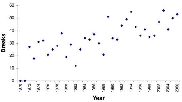
For the analysis, a homogeneous group of pipes was extracted that comprises of all 6” (150 mm) unlined cast iron (UCI) pipes installed in the 10-year period 1951-60. In total 897 individual pipe records (we respected the utility’s definition of ‘individual pipe’ as was reflected in the database) with total length of about 125 km were identified. The shortest and longest pipes on record were about 2.4 m and 663 m, respectively. Climate data for the analysis years were obtained from Environment Canada. Analysis was conducted on breaks recorded between 1970-2006 since no breaks were identified prior to 1970 for this specific group. Further, the group of pipes consists of only breaks that were specifically identified as circular, longitudinal or corrosion hole. Aggregate breakage data are illustrated in Figure 1. The availability of a relatively long breakage history enabled us to test the model on different time periods.

0 10 20 30 40 50 60 1970 1972 1974 1976 1978 1980 1982 1984 1986 1988 1990 1992 1994 1996 1998 2002 2004 2006 Year B reaks

We ran the model with several hundred different scenarios, where we varied training period durations, validation period durations, full dataset, partial datasets (e.g., only pipes with at least x breaks in the training period, only pipes at least 20 m long), combinations of group and pipe-level covariates, etc. The following general trends emerged:

• A longer duration training period improved STDEt, slightly improved STDEv, but did not affect rank correlation

• Longer validation period did not affect STDEv or rank correlation but improved the forecast of aggregate breaks.

• Climate covariates applied at group level improved STDEt slightly, but degraded it when applied at the pipe level.

• Usage of climate covariates at pipe level in training period tended to mitigate a large over-prediction in the validation but did not improve rank correlation.

• Length covariate did not have a significant impact on STDEt or STDEv or rank correlation.

• PKNOF covariate significantly improved STDEv.

• Usage of HSPC covariate at group and pipe levels improves STDEt and rank correlation, but improved STDEv only at pipe level.

• Pipe-level constant somewhat improved STDEv and rank correlation.

• Applying the model only to pipes with length of at least 20 m, or only to pipes that experienced at least 1 or 2 or 3 breaks during the training period had no significant impact.

• Scenarios with the lowest STDEt did not necessarily correspond to scenarios with the lowest STDEv, which in turn did not correspond to those with the highest rank correlation values.

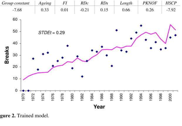
As an illustration we describe here the results of a scenario that used the entire dataset (897 pipes) over the entire available breakage history, i.e., training period of 1970-2001 and validation period of 2002-2006. All covariates were used at the group level, except for the pipe-level constant, which was of course used at pipe level. The coefficients obtained from training are presented in Figure 2, along with an illustration of the trained model (aggregate breaks) with respect to the observed data. Pipe-level constant

coefficients are not shown because by definition each pipe has a unique coefficient. An examination of the coefficients reveals that background ageing is proportional to cubic root (power of 0.33) of time. The impact of climate covariates on the model is inconsistent. Freezing index (FI) showed little impact, snapshot rain deficit (RDs) appeared to have a more significant impact, but cumulative rain deficit (RDc) showed a relative larger impact but in a counter intuitive direction (negative coefficient). Water mains of this water utility are typically buried at a depth of 2.4 m, which may explain the insignificant impact of FI, but not the negative sign of RDc. The negative coefficient of HSCP reflects the fact that hotspot anodes act to reduce breakage intensity. The positive sign of PKNOF may point to a “worse than old” condition (in repairable systems three repair-related conditions are observed, “good as new”, “good as old” and “worse than old”). The length covariate in this case study was taken as the loge of pipe length, which means that length to the power of approximately 2/3 is the influencing factor.

The forecast for the validation period was generated by running the scenario 20 times since the forecast is typically probabilistic. The validation standard error was 0.37 <

STDEv < 0.44. Spearman rank correlation coefficient was between 0.16 and 0.27. In

addition, we tested how well the forecast could identify the highest breaking pipes in the entire validation period. Results are presented in Table 1.

Group constant Ageing FI RDc RDs Length PKNOF HSCP

-7.68 0.33 0.01 -0.21 0.15 0.66 0.26 -7.92 0 10 20 30 40 50 60 1970 1972 1974 1976 1978 1980 1982 1984 1986 1988 1990 1992 1994 1996 1998 2000 Year B rea ks STDEt = 0.29

Figure 2. Trained model.

Table 1.

How many pipes observed with n breaks or more in the validation period did the model actually identify?

n Number of pipes observed Number of pipes identified

5 1 0

4 4 0 - 2

3 13 0 - 4

2 40 6 - 10

1 189 61 - 72

For comparison, it should be noted that the probability of drawing at random one correct pipe out of 897 is about 0.1%. The probability of drawing at random 4 correct pipes of 897 and “hitting more than zero of them correctly is about 1.8% (probability of “hitting” more than 1 is about 0.1%). Similarly, probability of “hitting” more than 2 when drawing 13 pipes of 897 is about 0.06%. Probability of hitting more than 5 when drawing 40 pipes

out of 897 is about 0.7%. And finally, probability of “hitting more than 60 times when drawing at random 189 pipes out of 897 is about 0.003%.

5. Summary and conclusions

A non-homogeneous Poisson process based model, which considers three classes of covariates, pipe-dependent, time-dependent and pipe and time dependent is proposed to forecast water main breaks. It is proposed that analyses should be conducted at two levels namely, at group and pipe levels to avoid the implication that all covariates have the same impact on all pipes. Break data analysis involves two steps: first step involves the training the model (discern coefficients) on data of T years (training period) and the second step involves simulation where discerned coefficients are used to forecast breaks in

subsequent V years (validation period).

Preliminary results, reflected in the case study, indicate the proposed model has good potential. A method needs to be developed to select the best combination for a given dataset since the model can be applied with various combinations of covariates (i.e., at pipe-level, at group level, etc.).

Acknowledgement

This paper presents interim results of a research project, which is co-sponsored by the AwwaRF, the NRC and water utilities from the United States and Canada. The authors wish to acknowledge the invaluable help provided by Dr. Ahmed Abdel Akher at the NRC.

References

Andreou, S. A., Marks, D. H., and Clark, R. M. (1987). “A new methodology for modeling break failure patterns in deteriorating water distribution systems: Theory.” Advance in Water Resources, 10, 2-10. Boxall, J. B., A. O’Hagen, S. Pooladsaz, A. Saul, and D. Unwin, (2007). Estimation of burst rate in water

distribution mains”, Proceedings of the Institution of Civil Engineers, Water Management I60, Issue

WM2, pp 73-82. June.

Constantine, A. G., and Darroch, J. N. (1993). “Pipeline reliability: stochastic models in engineering technology and management.” S. Osaki, D.N.P. Murthy, eds., World Scientific Publishing Co. Dridi, L,. Mailhot, A., Parizeau, M., and Villeneuve J.P. (2005) “A strategy for optimal replacement of

water pipes integrating structural and hydraulic indicators based on a statistical water pipe break model”. Proceedings of the 8th International Conference on Computing and Control for the Water

Industry, U. of Exeter, UK, September, 65-70.

Giustolisi, O., Laucelli, D, and Savic D. A., (2005). “A decision support framework fro short time planning of rehabilitation”, Proceedings of Computer and Control in Water Industry (CCWI), (1), 39-44.

Jarrett, R. O. Hussain, and J. Van der Touw (2003). “Reliability assessment of water pipelines using limited data”, OzWater, Perth, Australia.

Kleiner, Y. and Rajani, B. (2001). “Comprehensive review of structural deterioration of water mains: statistical models”. Urban Water, (3), 131-150.

Kleiner, Y. and Rajani, B. (2004). “Quantifying effectiveness of cathodic protection in water mains: theory,” Journal of Infrastructure Systems, ASCE, 10,(2), 43-51.

Le Gat, Y. (2007). “Extending the Yule Process to model recurrent failures of pressure pipes”,Private

communication.

Mailhot, A., A. Paulin, and Villeneuve J-P, (2003). “Optimal replacement of water pipes”, Water

Pintér, J. D. (2005). “LGO: A Model Development and Solver System for Continuous Global

Optimization”

, Pintér Consulting Services, Inc., Halifax, NS, Canada.

Røstum, J. (2000). “Statistical modelling of pipe failures in water networks”. PhD thesis, Norwegian University of Science and Technology, Trondheim, Norway.

S. Park and G. V. Loganathan (2002). “Optimal pipe replacement analysis with a new pipe break prediction model” Journal of the Korean Society of Water and Wastewater, 16/6, pp. 710-716.

Watson, T.G., C.D. Christian, A. J., Mason, M. H. Smith, and R. Meyer (2004). “Bayesian-based pipe failure model”, Journal of Hydroinformatics, IWA publishing, 06.4, pp 259-264.