Cohérences locales adaptatives dans les réseaux de contraintes.

N◦d’ordre : 2735

THÈSE DE DOCTORAT

Préparée dans le cadre d’une cotutelle entre

l’Université Mohammed V & l’Université de Montpellier

présentée par

Mohamed Amine B

AL AFREJ

Discipline : Sciences de l’Ingénieur

Spécialité : Informatique

Cohérences locales adaptatives dans les

réseaux de contraintes

Soutenue le 24 Novembre 2014, devant le jury composé de :

Président :

M. Mohammed BENKHALIFA, PES, FSR, Université Mohammed V, Rabat

Examinateurs :

M. Christian BESSIERE, DR-CNRS, CNRS-LIRMM, Montpellier

M. El Houssine BOUYAKHF, PES, FSR, Université Mohammed V, Rabat M. Adil KABBAJ, PES, Institut National des Statistiques et

d’Economie Appliquée, Rabat M. Redouane EZZAHIR, PH, ENSA, Université Ibn Zohr, Agadir M. Joël QUINQUETON, Pr, LIRMM, Université de Montpellier

faculté des sciences, 4 Avenue Ibn Battouta B.P. 1014 RP, Rabat-Maroc Tel:+212 (0) 37 77 18 34/35/38, Fax:+212 (0) 37 77 42 61

iii

Acknowledgements

The work presented in this thesis was carried out in the Laboratoire d’Informatique Mathé-matiques appliquées Intelligence Artificielle et Reconnaissance de Formes (LIMIARF), Faculty of Science, University Mohammed V, Rabat, Morocco and the Laboratoire d’Informatique, de Robo-tique et de Microélectronique de Montpellier (LIRMM), University of Montpellier, France. Under the joint supervision of Professor El-Houssine BOUYAKHF(PES, Faculty of sciences, University

Mo-hammed V, Morocco) and Professor Christian BESSIERE(DR, Centre National de Recherche Scien-titique, France). This thesis has been done in a joint supervision ’cotutelle’ between University Mohammed V, Morocco and University of Montpellier, France under the financial support of the scholarship of the programme Averroés funded by the European Commission within the frame-work of Erasmus Mundus.

I am greatly indebted to my supervisors Professor El-Houssine BOUYAKHF(PES, Faculty of sci-ences, University Mohammed V, Morocco) and Professor Christian BESSIERE(DR, Centre National de Recherche Scientitique, France) for their patience and support. I appreciate all their contribu-tions of time, ideas and guidance to make my Ph.D experience productive and stimulating.

I also would like to express thanks to Professor Mohammed BENKHALIFA(Faculty of sciences, University Mohammed V, Morocco) for accepting to preside the jury of my dissertation.

I gratefully acknowledge my reviewer Professor Adil KABBAJ(PES, Institut National des Statis-tiques et d’Economie Appliquée, Rabat, Morocco) for her constructive comments on this thesis.

I gratefully acknowledge my reviewer Professor Professor Redouane EZZAHIR (Professeur Ha-bilité, Université Ibn Zohr, Agadir, Morocco) for her constructive comments on this thesis.

I would like to record my gratitude to Professor Joël QUINQUETON, (Professor, University of

Montpellier, France) for his thorough examination of the thesis.

I am very grateful to all the people who directly or indirectly influenced my work during the last three years in Montpellier. Especially I would like to thank past and present members of coconut team. My sincere thanks also goes to the past and present members of the LIMIARF laboratory for their moral support. I also owe my deepest gratitude to professor Gilles TROMBITTONIand professor Remi COLETTAfor their collaboration, supervision and support.

This experience would not have been possible without the Averroès exchange programme. I would like to thank all the members of the Averroès exchange programme coordination. Especially I would like to thank Nathalie LAPUYADE, Elodie ERNOULTand Ambar GONZALEZBOUAB.

I would also like to thank all my friends who makes my stay in Montpellier a very pleasant one. My final words are reserved to my family: my beloved parents, my two sisters, my brother-in-law and my two nephews. Thank you for your whole support and unconditional love. Thank you very much.

Abstract

This thesis deals with adapting the level of consistency during solving a constraint satisfaction

problem (CSP). It focuses on the use of local consistency properties stronger than arc consistency (AC) to improve the CSP solving efficiency. Local consistency properties stronger than arc

consis-tency are generally expensive to maintain in a constraint network. Therefore, these local consisten-cies are seldom used in practice. This thesis gives several contributions to benefit from the filtering power of local consistencies stronger than AC while avoiding the high cost of maintaining them in the whole constraint network and throughout the search. First, we introduce the parameterized

local consistency (p-LC), an original approach that allows us to define intermediate levels of

consis-tency between AC and a local consisconsis-tency LC stronger than AC. Then, we present the instantiation of the parameterized local consistency approach to maxRPC and SAC, two consistencies stronger than AC. This leads to two parameterized consistencies, namely p-maxRPC and p-SAC. After giv-ing the definitions of p-maxRPC and p-SAC, we present the algorithm p-maxRPC3, that achieves p-maxRPC and the algorithm p-SAC1, for achieving p-SAC in a constraint network. We show exper-imentally that maintaining an intermediate level of consistency p-LC, can give a good compromise between filtering power and the computational cost of maintaining this level of consistency. We also show that for each instance of CSP we can find a parameter that gives this good compromise. The parameterized local consistency approach does not specify how the parameter can be chosen

a priori. Hence, we propose two techniques to automatically adjust the parameter p. In fact, both

techniques don’t use a single parameter, but several parameters. Each parameter is mapped to a part of the problem and it is automatically and locally adjusted during search. Finally, we propose POAC1, the first algorithm achieving partition-one-AC (POAC) in a constraint network. We com-pare POAC to SAC and we found that POAC converges faster than SAC to the fixed point due to its ability to prune values from all variable domains when being enforced on a given variable. Based on this observation, we proposed APOAC, an adaptive version of POAC, that monitors the number of variables on which to enforce POAC.

Keywords: Artificial Intelligence (AI), Constraint Programming (CP), Constraint Satisfaction

Problem (CSP), Local Consistency, Adaptive Local Consistency.

Résumé

Cette thèse traite de l’adaptation du niveau de cohérence locale au cours de la résolution d’un problème de satisfaction de contraintes (CSP). En particulier, nous nous intéressons à l’utilisation des propriétés de cohérence locale plus fortes que la cohérence d’arc (AC) pour gagner en efficacité de résolution d’un CSP. Les cohérences plus fortes que AC sont généralement coûteuses à main-tenir dans un réseau de contraintes. Par conséquent, elles sont rarement utilisées en pratique. Cette thèse apporte plusieurs contributions qui permettent de bénéficier de la puissance de filtrage de ces cohérences fortes tout en évitant le coût élevé de les maintenir dans tout le réseau de contraintes. Premièrement, nous introduisons la cohérence locale paramétrée (p-LC), une approche originale qui permet de définir des niveaux de cohérence intermédiaires entre AC et une de cohérence locale LC, plus forte que AC. Puis, nous présentons l’instanciation de cette approche à maxRPC et SAC, deux cohérences plus fortes que AC. Il en découle deux cohérences paramétrées, à savoir p-maxRPC et p-SAC. Ensuite, nous présentons l’algorithme p-maxRPC3, qui réalise p-maxRPC et l’algorithme p-SAC1, pour réaliser p-SAC dans un réseau de contraintes. Deuxièmement, nous montrons ex-périmentalement que maintenir un niveau de cohérence intermédiaire p-LC, peut donner un bon compromis entre puissance de filtrage et coût de calcul nécessaire pour maintenir ce niveau de co-hérence. En outre, nous montrons que pour chaque instance de CSP il est possible de trouver un paramètre adéquat qui donne ce bon compromis. L’approche de cohérence paramétrée ne précise pas comment le paramètre peut être choisi a priori. Nous proposons donc deux techniques qui per-mettent d’ajuster automatiquement le niveau de cohérence paramétrée p-LC. Ces deux techniques utilisent plusieurs paramètres à la fois. Chaque paramètre est associé à une partie du problème et s’adapte automatiquement et localement au cours de la résolution. Finalement, nous proposons POAC1, le premier algorithme pour établir partition-one-AC (POAC) dans un réseau de contraintes. Puis, en comparant POAC à SAC nous constatons que POAC converge au point fixe plus rapidement que SAC. Sur la base de ce constat, nous proposons APOAC, une version adaptative de POAC qui contrôle le nombre de variables sur lesquelles POAC est appliqué.

Mots clefs : Intelligence Artificielle (AI), Programmation par Contraintes (CP), Problème de

Sat-isfaction de contraintes (CSP), Consistance Locale, Consistance Locale Adaptative.

Résumé étendu

La programmation par contraintes est un formalisme puissant permettant la modéli-sation de problèmes combinatoires puis leur résolution par des méthodes génériques. Il a été appliqué avec succès à de nombreux domaines de la vie réelle, telles que la planifica-tion des satellites [Bensana et al., 1999], l’analyse de circuit [De Kleer and Sussman, 1980] ou encore l’allocation des fréquences radio [Cabon et al., 1999].

Le succès de ce formalisme est dû à son expressivité qui permet à l’utilisateur de mod-éliser le problème d’une manière naturelle, ainsi qu’à l’efficacité des méthodes de résolu-tion génériques développés pour résoudre tout problème exprimé sous forme de problème de satisfaction de contraintes. Modéliser un problème revient à l’exprimer sous forme d’un réseau de contraintesN = (X, D, C), oùXreprésente l’ensemble des variables, c’est à dire les inconnues du problème.Dreprésente l’ensemble des domaines, chaque variablex_i∈X

possède un domaineD(xi)∈Dqui représente l’ensemble des valeurs que peut prendre la variable. EtCun ensemble de contraintes exprimées de façon naturelle pour restreindre les combinaisons de valeurs que pourront prendre simultanément des variables deX. Le

problème de satisfaction de contraintes (CSP), est le problème générale de décider si un réseau de contraintesN = (X, D, C)possède des solutions, c’est à dire des combinaisons de valeurs, attribuant à chaque variable une valeur de son domaine respectif et satisfaisant toutes les contraintes du problème.

Le problème de satisfaction de contraintes (CSP) étant NP-complet, il est généralement résolu grâce à une méthode qui parcoure l’espace de recherche, en alternant entre une phase d’exploration (aussi appelée branchement ou instanciation) et une phase de prop-agation (aussi appelée filtrage). L’exploration de l’espace de recherche est organisée sous forme d’un arbre où chaque nœud représente l’instanciation d’une variable à une valeur de son domaine et les branches sortant d’un nœud représentent les choix d’instanciations possibles pour la variable suivante. Après chaque branchement (instanciation d’une

able à une valeur), la phase de propagation est exécutée afin d’inférer des inconsistances locales. Une inconsistance locale est une valeur ou combinaison de valeurs ne pouvant appartenir à aucune solution. La détection de ces inconsistances locales permet d’éviter l’exploration de sous espaces de recherche ne contenant pas de solutions et ainsi réduire considérablement la taille de l’espace de recherche à parcourir.

Les inconsistances locales sont principalement inférées grâce aux propriétés de con-sistance locale. La concon-sistance d’arc, introduite par Mackworth, est la plus connue des consistance locale et la plus utilisée en pratique par les solveurs. Elle permet de garantir que chaque valeur de chaque variable soit compatible avec chacune des contraintes prise indépendamment. En d’autres termes, la consistance d’arc garantit pour chaque valeurvi de chaque variablexiet pour chaque contrainteci∈Cprise indépendamment, qu’il y a au moins une combinaison de valeurs qui peuvent être prises simultanément par les variables impliquées dansciet où la variablexiprend la valeurvi.

Historiquement, Le Forward Checking (FC) [Haralick and Elliott, 1979] été considéré comme la meilleure technique à utiliser pour inférer et supprimer des valeurs localement inconsistantes au cours de la résolution d’un CSP. Le FC est une forme partielle de la con-sistance d’arc, elle garantie la concon-sistance d’arc uniquement pour les contraintes impli-quant des variables déjà instanciées. Par conséquent, AC peut détecter plus de valeurs inconsistantes que FC. En 1994, il a été démontré dans [Sabin and Freuder, 1994] que l’utilisation de la consistance d’arc dans sa forme complète pour éliminer les valeurs locale-ment inconsistantes est un choix intéressant lors de la résolution de problèmes difficiles de grande taille. Peu de temps après, d’autres études ont également confirmé ce résul-tat [Bessière and Régin, 1996; Grant and Smith, 1996]. Ainsi, le maintien de la consistance

d’arc (MAC) [Sabin and Freuder, 1994] est devenue la méthode la plus largement utilisée

pour résoudre le problème de satisfaction de contraintes.

Plusieurs propriétés de consistance locale ont été proposées par la communauté de programmation par contraintes [Berlandier, 1995; Freuder and Elfe, 1996; Debruyne and Bessiere, 1997; Debruyne and Bessière, 1997; Bessiere, 2006], et des relations "d’ordre" existent entre plusieurs d’entre elles [Debruyne and Bessière, 1997] : les unes peuvent détecter et supprimer plus de valeurs inconsistantes que les autres. Cependant, choisir de maintenir une consistance locale ’A’ plus forte qu’une autre ’B’ au cours de la résolu-tion d’un CSP, peut garantir la réducrésolu-tion de la taille de l’espace de recherche, mais cela n’implique pas la minimisation du temps de résolution du problème, car dans un tel choix il y a un compromis à faire entre la capacité d’une propriété de consistance locale à supprimer des valeurs et la complexité temporelle des algorithmes qui permettent de l’atteindre.

Dans cette thèse nous proposons de maintenir une forme de consistance locale adap-tative qui peut exploiter la puissance de filtrage des propriétés de consistance locale plus fortes que l’AC tout en évitant le coût élevé de maintenir ces consistances dans tout le réseau de contraintes. Notre objectif est de trouver un compromis meilleur que celui

xiii

obtenus par le maintien de la consistance d’arc ou le maintien d’une consistance plus forte LC.

Le premier chapitre de cette thèse rappelle les définitions de base et survole les méth-odes de résolution et les consistances locales proposées dans la littérature. Dans le deux-ième chapitre de cette thèse, nous définissons la notion de stabilité pour les valeurs. Une notion originale qui n’est pas basée sur les caractéristiques de l’instance à résoudre, mais basée sur l’état de l’algorithme de propagation de la consistance d’arc pendant son exé-cution. En se basant sur cette notion, nous proposons le concept de consistance locale

paramétrée, une approche originale qui permet d’ajuster le niveau de consistance

lo-cale utilisé pour résoudre une instance donnée. Une consistance paramétrée p-LC main-tient un niveau intermédiaire de consistance entre l’AC et une autre consistance LC plus forte que la consistance d’arc. Le pouvoir d’élagage (capacité à détecter des valeurs in-consistantes) de p-LC dépend du paramètre p. Cette approche nous permet de trouver un bon compromis entre la puissance d’élagage d’une consistance locale et le coût en terme de temps CPU des algorithmes qui permettent de l’atteindre. Nous appliquons le concept de consistance paramétrée p-LC aux deux propriétés de consistance locale plus fortes que l’AC les plus connues, qui ne modifient pas la structure du réseau, à savoir maxRPC et SAC. Nous décrivons l’algorithme p-maxRPC3, basé sur maxRPC3 [Balafoutis et al., 2011b], qui réalise la p-max consistance de chemin restreinte ainsi que l’algorithme p-SAC1, qui réalise la p-singleton consistance d’arc. Nous évaluons expérimentalement l’intérêt d’utiliser la consistance locale paramétrée. Et nous montrons qu’en faisant le bon choix du paramètre p, nous profitons du coût réduit de calcul de la consistance d’arc et l’efficacité d’élagage de la consistance forte LC. Dans le meilleur des cas, un solveur qui maintient un niveau de consistance intermédiaire p-LC explore le même nombre de nœuds qu’en maintenant LC avec un nombre de vérification de contraintes aussi réduit que lors du maintien d’ AC, ce qui entraine une baisse de temps CPU de résolution com-paré aux temps obtenus utilisant AC ou LC.

Le troisième chapitre complète le deuxième en proposant deux techniques pour ren-dre une consistance paramétrée adaptative de manière automatique et dynamique. En effet, le chapitre 2 définit le concept de consistance paramétrée et montre que le bon choix du paramètre permet d’avoir un bon compromis entre filtrage et coût de calcul. Mais ne donne pas comment ce paramètre peut être choisit. Ainsi le troisième chapitre comble ce manque et propose deux techniques pour adapter dynamiquement et locale-ment le paramètrepdans le but de résoudre le problème plus rapidement que AC et la consistance forte LC. Au lieu d’utiliser un seul paramètreppendant toute la recherche et pour l’ensemble du réseau de contraintes, nous proposons d’utiliser plusieurs paramètres locaux et d’adapter le niveau de consistance locale en ajustant automatiquement et dy-namiquement la valeur des différents paramètres locaux pendant la recherche. L’idée est de concentrer l’effort de propagation en augmentant le niveau de consistance dans les parties les plus difficiles de l’instance. Nous déterminons ces parties difficiles grâce aux heuristiques basées sur les conflits tel que le poids d’une contrainte et le degré pondéré

d’une variable [Boussemart et al., 2004]. La première technique que nous proposons, appelé constraint-basedap-LC, attribue un paramètrep(ck) à chaque contrainteck. Et chaque paramètrep(ck)est corrélé au poids de la contrainte associée ck. La deuxième technique que nous proposons est appelé variable-basedap-LC, elle consiste à attribuer un paramètre p(xi), à chaque variable xi, corrélé au degré pondéré de cette variable

xi[Boussemart et al., 2004]. L’objectif des deux techniques est d’appliquer un niveau de consistance plus élevé dans les parties du problème où les contraintes sont les plus act-ifs. Nous appliquons ces deux techniques à p-maxRPC et nous évaluons expérimentale-ment ces deux techniques. Nous pouvons constater que ces deux techniques que nous proposons pour l’ adaptation automatique du niveau de consistance locale pendant la recherche sont efficaces en pratique et peuvent surpasser AC et la consistance forte LC. En comparant ces deux techniques nous observons que, bien que la version constrainte-based est plus fine dans sa conception, la version variable-constrainte-based est souvent plus rapide. En effet, à cause des valeurs initiales des poids des contraintes, tous les paramètres lo-caux prennent la valeur0, donc la constraint-based commence la résolution en appliquant uniquement l’AC et commence à exploiter la puissance de filtrage de la consistance forte LC seulement après le premier échec de MAC. Alors que la version variable-based ne souf-fre pas de cet inconvénient et peut bénéficier de la puissance de filtrage de la consistance forte des le début de la recherche.

Dans le quatrième chapitre de cette thèse, nous rappelons la définition de la Partition-One-AC (POAC), une consistance, basée sur les tests de singleton, plus forte que SAC. Puis nous proposons POAC1, le premier algorithme pour atteindre POAC dans un réseau de contraintes. En suite, nous comparons POAC et SAC et nous montrons, qu’en plus d’être plus forte que SAC, POAC converge au point fixe plus rapidement que SAC. Sur la base de ce constat, nous proposons une version adaptative de POAC (APOAC) où le nombre de variables traitées est adapté dynamiquement et automatiquement au cours de la recherche d’une solution. APOAC représente une approche différente de celles présentées précédem-ment. Au lieu d’attendre que les échecs se produisent pour identifier les parties difficiles du problème et pouvoir bien profiter de la puissance de filtrage des consistances forte, nous divisons la résolution du problème en plusieurs cycles, chacun constitué d’une phase d’entraînement suivit d’une phase d’exploitation et nous nous basons sur l’ apprentis-sage effectué dans chaque phase d’entraînement pour décider de la puissance de filtrage à appliquer dans la phase d’exploitation qui suit. Nous avons expérimenté l’algorithme POAC1 et trois variantes de la version adaptative APOAC et nous avons montré que la POAC améliore SAC et que les variantes adaptatives améliorent AC dans les instances difficiles.

Contents

1.2 Definition of the constraint satisfaction problem (CSP) . . . 24

1.2.1 Example of CSP . . . 25 1.2.2 Modelling . . . 26 1.3 Solving methods . . . 28 1.3.1 Chronological Backtracking (BT) . . . 29 1.3.2 Look-back methods . . . 31 1.3.3 Look-ahead methods . . . 32 1.4 Local Consistencies . . . 32

1.5 arc consistency (AC) . . . 34

1.5.1 Definition . . . 34

1.5.2 AC algorithms . . . 35

1.6 max-Restricted Path Consistency (maxRPC) . . . 39

1.6.1 Definition . . . 39

1.6.2 maxRPC Algorithms . . . 40

1.7 Singleton Arc Consistency (SAC) . . . 46

1.7.1 Definition . . . 46

1.7.2 SAC Algorithms . . . 48

1.8 Partition-One-AC (POAC) . . . 50

1.8.1 Definition . . . 50

1.8.2 The POAC algorithm . . . 50

1.9 Summary . . . 50

2 Parametrized Local Consistencies 51 2.1 Introduction . . . 52

2.2 Parameterized Consistency . . . 53

2.2.1 p-Stability concept . . . 53

2.2.2 Constraint-based parameterized local consistencies . . . 55

2.2.3 Value-based parameterized local consistencies . . . 56

2.3 Parameterized maxRPC:p-maxRPC . . . 57

2.3.1 Definition . . . 57

2.3.2 p-maxRPC3 algorithm . . . 57

2.4 Parameterized SAC:p-SAC . . . 60

2.4.1 Definition . . . 60

2.4.2 p-SAC1 algorithm . . . 60

2.5 Experimental Evaluation . . . 62

2.6 Summary . . . 66

3 Adaptive Parametrized Local Consistencies 69 3.1 Introduction . . . 70

3.2 Adaptative Parameterized Local Consistency:ap-LC . . . 70

3.2.1 Constraint-Basedap-LC:apc-LC . . . 71

3.2.2 Variable-Basedap-LC:apx-LC . . . 71

3.3 Adaptative Parameterized maxRPC:ap-maxRPC . . . 72

3.3.1 Constraint-Basedap-maxRPC:apc-maxRPC . . . 72

3.3.2 Variable-Basedap-maxRPC:apx-maxRPC . . . 73

3.4 Experimental Evaluation ofap-maxRPC . . . 73

3.5 Summary . . . 75

4 Adaptive Singleton-based Consistencies 77 4.1 Introduction . . . 78

4.2 POAC . . . 79

CONTENTS xvii

4.2.2 Comparison of POAC and SAC behaviors . . . 80

4.3 Adaptive POAC . . . 82 4.3.1 Principle . . . 83 4.3.2 Computingki(j) . . . 84 4.3.3 Aggregation of theki(j)s . . . 85 4.4 Experiments . . . 85 4.5 Summary . . . 89 Conclusion 91 Bibliography 93 List of Figures 102 List of Tables 103

Introduction

Constraint Programming (CP) is a powerful formalism for modelling and solving

com-binatorial problems. It has been successfully applied to many areas of real life, such as satellite scheduling [Bensana et al., 1999], circuit analysis [De Kleer and Sussman, 1980] or frequency assignment [Cabon et al., 1999].

The success of this formalism is due to its expressiveness that allows the user to model the problem in a natural way, and the effectiveness of generic solving methods developed to solve problems expressed as constraint satisfaction problem. Model a problem is to formulate it as a constraint network N = (X, D, C), where X is the set of variables, i.e. the unknowns of the problem. Dthe set of domains, each variablexi∈Xhas a domain

D(xi)∈D, which represents all possible values for the variable. Ca set of constraints ex-pressed in a natural way restricting the combinations of values that can simultaneously take some variables inX. The constraint satisfaction problem (CSP), is the general task of deciding whether a constraint network N = (X, D, C)has solutions, i.e. combinations of values, assigning to each variable a value from its respective domain and satisfying all the constraints of the problem.

The constraint satisfaction problem being NP-complete, it is usually solved by a method that traverses the search space, alternating between an exploration phase (also called branching or instantiation) and a propagation phase (also called filtering or pruning). The exploration of the search space is organized as a tree where each node represents the in-stantiation of a variable to a value in its domain and branches out of a node represent alternative instantiation choices for the next variable. After each branching (instantiation of a variable to a value), the propagation phase is executed to infer local inconsistencies. A local inconsistency is a value or a combination of values that cannot belong to a solution. The detection of these local inconsistencies avoids exploring some subspaces containing no solutions and thus significantly reduces the size of the search space to explore.

Local inconsistencies are mainly inferred using the local consistency properties. Arc

Consistency (AC), introduced by Mackworth, is the most well known local consistency and

widely used in practice in the constraint solvers. It ensures that each value of each variable is consistent with each constraint taken independently. In other words, arc consistency guarantees for each valuevifor each variablexi, and for each constraintci∈Cinvolvingxi and taken independently, that there exist at least one combination of values that can take the variables involved inci, and where the variablexiis set tovi.

Forward Checking (FC)[Haralick and Elliott, 1979] was historically considered the best

technique to use to infer and remove some inconsistent values when solving a CSP. FC is a partial form of arc consistency, it guarantees arc consistency only for constraints involv-ing some variables already instantiated.Therefore, AC can detect more inconsistent values than FC. In 1994, it was shown in [Sabin and Freuder, 1994] that using complete arc

con-sistency to eliminate locally inconsistent values is an interesting choice when solving large

and difficult problems. Soon after, other studies have also confirmed this result [Bessière and Régin, 1996; Grant and Smith, 1996]. Since then, maintaining arc consistency (MAC) [Sabin and Freuder, 1994] became the most widely used method to solve constraint satis-faction problem.

Many local consistency properties have been proposed by the constraint programming community [Berlandier, 1995; Freuder and Elfe, 1996; Debruyne and Bessiere, 1997; De-bruyne and Bessière, 1997; Bessiere, 2006], and there is order relationships [DeDe-bruyne and Bessière, 1997] between several of them, i.e. some of them can detect and remove more inconsistent values than other. However, choosing to maintain a local consistency ’A’ stronger than another ’B’ for solving a CSP, can ensure the reduction of the search space size, but that does not mean minimizing the solving time. In fact, choosing the right level of local consistency for solving a problem requires finding the good trade-off between the ability of this local consistency to remove inconsistent values, and the cost of the algorithm that enforces it.

In this thesis we propose to maintain an adaptive form of local consistency which can benefit the filtering power of local consistency properties stronger than AC, while avoiding the high cost of maintaining these local consistencies in the whole constraint network. Our goal is to find a compromise better than that achieved by maintaining arc consistency or maintaining a stronger consistency LC.

First, we introduce parameterized local consistency (p-LC), a general approach that de-fines intermediate levels of consistency between AC and a local consistency LC, stronger than AC. The filtering power of such consistency changes according to a parameter p. Then, we present an instantiation of the parameterized consistency approach to maxRPC and SAC, two consistencies stronger than AC. This leads to two parameterized consisten-cies, namely p-maxRPC and p-SAC. we present the algorithm p-maxRPC3, that achieves p-maxRPC and the algorithm p-SAC1, for achieving p-SAC in a constraint network.

Secondly, We shows experimentally that maintaining an intermediate consistency be-tween AC and a stronger locale consistency LC, can give a better compromise than

main-21

tain AC or LC. We also show that for each instance of CSP we can find a suitable parameter that gives a good compromise. However, this approach does not show how the parameter can be selected a priori. Hence, we propose two techniques to automatically adjust the parameter p. In fact, both techniques don’t use a single parameter, but several parame-ters. Each parameter is mapped to a part of the problem and it is automatically and locally adjusted during search. Both techniques were tested and the results show that adapt lo-cally and dynamilo-cally, the parameterized consistency during the resolution gives generally a good compromise between filtering power and computation cost.

Finally, we propose POAC1, the first algorithm to achieve partition-one-AC (POAC) in a constraint network. We compare POAC to SAC and we found that POAC converges faster than SAC to the fixed point. Based on this observation, we proposed APOAC, an adap-tive version of POAC. APOAC involves dividing the solving in several solving cycles. Each solving cycle consisting of a learning phase followed by an exploitation phase. During the learning phase APOAC decides the filtering power to be applied in the exploitation phase that follows. Three APOAC variants were tested and the results show that APOAC improves AC in difficult instances.

The thesis is organized as follows. The first chapter (chapter 1) recalls the basic defi-nitions and gives a brief overview of the solving methods and the local consistencies pro-posed in the literature. In chapter 2, we define the notion of stability of values. Then, based on this notion, we propose parameterized local consistency, an original approach that allows to define levels of local consistencyp-LC of increasing strength between arc consistency and a given strong local consistency LC. After that, we apply this approach to the cases where LC is max restricted path consistency or singelton arc consistency and we describe the algorithmp-maxRPC3, that achievesp-max restricted path consistency and the algorithmp-SAC1, for achievingp-singleton arc consistency. Finally, we experimen-tally assess the interest of parameterized local consistency that allows us to find a good trade-off between the pruning power of the local consistency and the computational cost of the algorithms that achieves it.

In chapter 3, we propose constraint-basedap-LC and variable-basedap-LC, two

adap-tive variants ofp-LC which adapts dynamically and locally the level of local consistency during search. Then we apply this adaptive variants to the case where LC is max restricted path consistency and we experimentally assess the practical relevance of adaptive param-eterized local consistency. In chapter 4 we present POAC1, an algorithm that enforces partition-one-AC efficiently in practice. Then we show that POAC converges faster than SAC to the fixpoint due to its ability to prune values from all variable domains when being enforced on a given variable. Based on this observation, we propose APOAC, an adaptive version of POAC. It involves dividing the search in several search cycles, each consisting of a learning phase followed by an exploitation phase. During the learning phase APOAC decides the filtering power to be applied in the exploitation phase that follows (i.e., the number of variables on which to perform singleton tests). Finally, we show experimentally that APOAC improves AC in difficult instances.

C

1

Background

Constraint programming represents one of the closest approaches computer science has yet made to the Holy Grail of programming: the user states the problem, the computer solves it.

EUGENEC. FREUDER

Preamble

Constraint programming is a powerful paradigm for modeling and solving combina-torial problems. It provides total separation between modeling and solving a problem. once modeled as a constraint satisfaction problem (CSP), the problem can be solved by a generic method. The most efficient and the most used solving methods consist in performing a depth-first traversal of a search tree and use local consistencies proper-ties to prune subtrees containing no solutions. Generally, the same property of con-sistency is used throughout the resolution for all the problem instances. In this thesis we are interested in adapting the level of consistency during the resolution of a con-straint satisfaction problem. The goal is to benefit from the pruning power of the local consistencies stronger than arc consistency while avoiding the high cost to maintain these strong consistencies in the whole constraint network. In this chapter we give the basic definitions for the constraint satisfaction problem, and a brief overview of the different methods used to solve a constraint satisfaction problem. Then we present the

local consistencies we used to test the algorithms we developed to adapt the level of consistency during solving a CSP.

Contents

1.1 Introduction . . . 24 1.2 Definition of the constraint satisfaction problem (CSP) . . . 24 1.3 Solving methods . . . 28 1.4 Local Consistencies . . . 32 1.5 arc consistency (AC) . . . 34 1.6 max-Restricted Path Consistency (maxRPC) . . . 39 1.7 Singleton Arc Consistency (SAC) . . . 46 1.8 Partition-One-AC (POAC) . . . 50 1.9 Summary . . . 50

1.1 Introduction

Constraint programming formalism, presented by Montanari in 1974, has been used successfully to model and solve many types of combinatorial problems like satellite scheduling [Bensana et al., 1999], circuit analysis [De Kleer and Sussman, 1980] or fre-quency assignment [Cabon et al., 1999]. The success of this formalism is due to its ex-pressiveness that allows the user to model the problem in a natural way, as well as the effectiveness of the algorithms developed for solving problems modelled as constraint sat-isfaction problem. This chapter provides a formal definition of the constraint satsat-isfaction problem in section 1.2, and gives some problem examples. Then it gives how a problem can be modelled and shows that many models can be founded for the same problem. The sec-tion secsec-tion 1.3 provides a brief overview of the different methods used to solve a problem and the section 1.4 presents the local consistencies properties on which we were interested and describes the algorithms enforcing these consistencies used in our experiments.

1.2 Definition of the constraint satisfaction problem (CSP)

In this thesis, we mainly focus on the finite discrete constraint satisfaction problem (CSP). A Constraint network (N) is defined by a set of variables, a set of domains and a set of constraints. Each domain represents the set of the possible values for a variable and each constraint restricts the combinations of values that can take simultaneously a subset of variables. The Constraint Satisfaction Problem (CSP) is to decide for a given constraint network whether it is possible to assign to each variable a value from its respective domain such that all constraints are simultaneously satisfied.

1.2. DEFINITION OF THE CONSTRAINT SATISFACTION PROBLEM (CSP) 25

Definition 1.1 (Constraint Network) A Constraint Network (N) is a triple(X, D, C)where: – X ={x1, ..., xn}is a set of variables that presents the unknowns of the problem,

– D ={D(x1), ..., D(xn)}is a set of domains,

– C = {c1, ..., ce} is a set of constraints. Each constraint ck is defined by a pair

(var(ck), sol(ck)), wherevar(ck)is an ordered subset ofX, and sol(ck) is a set of

combinations of values (tuples) satisfyingck. For a tuplet∈sol(ck),t[xi]denotes the

valueviassociated to the variablexi∈var(ck).

In this thesis we use n, dande to denote the number of variables in the constraint network, the maximum domain size and the number of constraints respectively. And we usecijto denote the binary constraint betweenxiandxj.

Definition 1.2 (Constraint satisfaction problem (CSP)) The problem of deciding whether

a constraint networkN = (X, D, C)has solutions is called the constraint satisfaction prob-lem (CSP), where variables presents the unknowns of the probprob-lem. The constraint satisfac-tion problem is NP-complete.

Definition 1.3 (Solution of a CSP) A solution of a CSP is an assignment of each variable of

the constraint network to a value in its domain such that all the constraints are simultane-ously satisfied.

In the following we useC(xi)to denote the set of constraintscj such thatxi∈var(cj) andΓ (xi)to denote the set of variablesxjinvolved in a constraint withxi.

Definition 1.4 (Degree of a variable) The degree of a variable, given byDeg(xi) =|C(xi)|,

is the number of constraints involving this variable in the constraint network.

Definition 1.5 (Constraint graph) A binary constraint network, composed by only binary

constraints, can be associated with a constraint graphG(V, E), where verticesVrepresents variablesXand edgesErepresents constraintsC.

1.2.1 Example of CSP

Constraint programming (CP) aims to solve difficult combinatorial problems expressed as constraint satisfaction problems. Before presenting how these difficult problems can be modelled and solved, this section gives two examples of difficult combinatorial problem. The first one is a real problem, called Radio Link Frequency Assignment problem. The sec-ond one is the academic N-queens problem. Then we give two CSP models of the academic N-queens problem.

The Radio Link Frequency Assignment Problem (RLFAP)

The Radio Link Frequency Assignment Problem (RLFAP) [Cabon et al., 1999] is a gen-eral task stems from real world problems in military telecommunication. RLFAP consists in assigning frequencies to a number of radio links in such a manner as to simultaneously satisfy a large number of constraints and use as few distinct frequencies as possible. In most cases the number of available frequencies is much smaller than the number of fre-quencies to be assigned.

As described in [Cabon et al., 1999], constraints can be of three different types: – Some links may already have a pre-assigned frequency

– The difference between the frequencies assigned to two different radio links must be equal to a constant imposed by technological constraints

– The difference between the frequencies assigned to two different radio links must be greater than a minimum distance.

The radio link frequency assignment problem is an NP-hard problem.

N-queens problem

According to [Freuder and Mackworth, 2006], the eight queens puzzle have been pro-posed in 1848 by the chess player Max Bazzel. The eight queens puzzle is an instance of the more general N-queens problem. The N-queens problem is to consider an N×N chess-board and ask if N queens can be placed on such a chess-board so that none of the queens can attack each other. A queen can attack an other if both of them are in the same horizontal, the same vertical, or in the same diagonal in the chessboard. Figure 1.1 shows a solution of the eight queens puzzle.

1.2.2 Modelling

To solve a problem using the constraint programming formalism, first it must be mod-elled as a constraint satisfaction problem. To model a problem, one must first choose the variables, i.e. the objects for which the user wants to find values in order to build a solution to his problem. In the example of N-queens, the variables could be the chessboard squares. Then one must define a domain for each variable, i.e. a set of values it can take. A square of the chessboard, may contain a queen or be empty. Then, describe the constraints that characterize the problem.

This section presents two models for the same N-queens problem, to show that for a given problem there may be several possible models.

N-queens problem (Model 1)

1.2. DEFINITION OF THE CONSTRAINT SATISFACTION PROBLEM (CSP) 27

Figure 1.1: A solution of the eight queens puzzle.

– X ={xi,j|i,j∈N×N}wherexi,jis the variable associated to the,ithrowjthcolumn, chessboard square.

Each variablexi,jtakes the valuer1if there is a queen in the rowi columnjand takes 0 otherwise.

– D ={D(xi,j)|i,j∈N×N}whereD(xi,j) ={0,1}∀i, j∈N×N. The constraints are:

– PN_j=1xi,j= 1, i = 1..N. (one queen, each row). – PN_i=1xi,j= 1, j = 1..N. (one queen, each column).

– xi,j+ xk,l≤1∀xi,j, xk,l, xi,j6= xk,landi + j = k + l. (queens must be on different rising diagonals).

– xi,j+ xk,l≤1∀xi,j, xk,l, xi,j6= xk,l andi − j = k − l. (queens must be on different de-scending diagonals).

N-queens problem (Model 2)

knowing that there can be only one queen per line. This second model combines a variable on each row.

– X ={xi|i = 1..N}wherexiis the variable associated to the,ithrow. And each variable may have a value in1..N.

– D ={D(xi)|i = 1..N}whereD(xi) ={1,...N}∀i∈1..N. The constraints are:

– {xi6= xj| i,j∈N×N, i6= j}. (queens must be on different columns).

– {|xi−xj|6=|i−j| | i,j∈N×N, i6= j}. (queens must be on different rising diagonals and different descending diagonals).

We have seen that for a same problem there may be several possible models. However, how the problem is modelled can have a substantial effect on how efficiently this problem can be solved. Several works were interested in improving the modeling of a problem and several techniques were proposed like adding symmetry breaking constraints, adding im-plied constraints to improve propagation and adding auxiliary variables to make it easier to state the constraints. An overview of all these techniques can be found in[Gent et al., 2006; Smith, 2006].

1.3 Solving methods

The separation between modeling and solving a problem represents one of the high-lights of the constraint programming formalism. Once the problem is modeled, it can be solved by a generic constraint solving method. Solving methods can be either complete or incomplete. Complete methods guarantees that a solution will be found if one exists, and can be used to prove that a CSP doesn’t have a solution if no solution exists. Incomplete methods are often effective to find a solution but cannot guarantee that a solution will be found if one exists, and cannot be used to prove that a CSP doesn’t have a solution.

Complete, or systematic solving methods performs a depth-first traversal of a search tree and use inference to avoid exploring some subtrees containing no solutions. While incomplete methods use a stochastic search based on heuristics and local search methods. In this thesis, we are not interested in the incomplete methods. For more details about these incomplete methods [Hoos and Tsang, 2006] may be consulted.

Figure 1.2 shows the search tree of the constraint network composed of the variables

x1,x2andx3with the respective domainsD(x1) = D(x2) ={v1, v2, v3}andD(x3) ={v1, v2}. The search tree is explored using the variable order(x₁, x₂, x₃). Each node represents an assignment of a variable to a value in its domain and the branches out of a node represent alternative choices, for the next variable, that may have to be examined in order to find a solution.

Backtracking algorithm is the most common generic algorithm for performing system-atic search and most complete methods for solving CSPs are based on the backtracking algorithm. We can distinguish two families of complete methods for solving CSP, namely look-back and look-ahead methods. Look-back methods aim to improve the backtracking algorithm using information extracted from the analysis of the partial instantiation when

1.3. SOLVING METHODS 29

Figure 1.2: Example of a Search tree for CSP

failure occurs. Look-ahead methods aim to improve the backtracking algorithm exploiting local consistencies to avoid such failure altogether. In this section we provide a detailed exposition of the Chronological backtracking algorithm then we give a description of this two families of complete solving methods.

1.3.1 Chronological Backtracking (BT)

Definition 1.6 (Assignment) An assignment is a pair(xi, vi), which means that variable

xi∈Xis assigned the valuevi∈D(xi).

Definition 1.7 (Instantiation) An instantiation I of an ordered set of variables S = {x1, x2, . . . , xk} is a sequence of assignments I = {(x1, v1), (x2, v2), . . . , (xk, vk)} of all the

variables of S. An instantiation can be represented by the tuple t = (v1, v2, . . . , vk) ∈

D(x1)×D(x2)× · · · ×D(xk) where ∀j ∈ 1..k, vj corresponds to the value assigned to the

jthvariable ofS.

Definition 1.8 (Locally consistent instantiation) An instantiation I of an ordered set of variablesS∈X is locally consistent if and only if it satisfy all the constraint ci ∈C such

thatvar(ci)⊆S.

Definition 1.9 (Solution) A solution of a constraint networkN = (X, D, C)is a locally con-sistent instantiation ofX.

The chronological backtracking [Golomb and Baumert, 1965; Bitner and Reingold, 1975] is a systematic search algorithm which proceeds to resolution by successive instan-tiation of variables in order to find a solution. So the algorithm tries to build a locally con-sistent instantiation ofX(a solution) by extending at each time a locally consistent instan-tiation ofkvariables, into another locally consistent instantiation ofk+1variables ofX. At each time the algorithm tries to instantiate an uninstantiated variable until all variables in

Xare instantiated. After each extension, of the instantiation by assigning a new variable, the algorithm checks if the new extended instantiation is always consistent with the con-straints involving its variables. If the extended instantiation is inconsistent, the algorithm attempts to assign the last variable to another value. If no value can be assigned to the last variable, the algorithm performs a backtrack to change the value assigned to the variable just before the last assigned variable.

Figure 1.3: Example of a Search tree for CSP

Figure 1.3 shows the nodes visited by the chronological backtracking when exploring the search tree of the constraint network composed of the variablesx1,x2andx3with the respective domainsD(x1) = D(x2) ={v1, v2, v3}andD(x3) ={v1, v2}and the constraints

{x16= x2, x26= x3}. After assigningv1tox1andv2tox2, i.e. I ={(x1, v1), (x2, v2)}, chrono-logical backtracking can detect the inconsistency of this instantiation (because does not satisfy the constraintx1 6= x2). It infers that this partial instantiation (I) cannot be ex-tended to a solution. Thus, BT will save the checks of consistency for both instantiations

1.3. SOLVING METHODS 31

The chronological backtracking algorithm, depicted in algorithm 1, tries to extend a lo-cally consistent instantiationIof a subset of variables inX, into a locally consistent instan-tiation of all the variables inX. The algorithm starts by checking if the locally consistent instantiationIis complete (line 2), i.e. all the variables inXare assigned. If it is, it prints

Ias a solution (line 3). If not, it selects an unassigned variablexi(line 5) and attempts to extendIby instantiatingxito a valueviin its domain (line 6). If the extended instantiation is locally consistent (line 7), the algorithm tries to extend the new instantiation by assign-ing a new variable (line 8). Otherwise (no value inD(xi)can extendsI), it returns back to change the value of the latest assigned variable in the instantiationI(line 9).

Algorithm 1: BT(I, X, D, C) 1 begin 2 if|I| = |X|then 3 printSolution(I); 4 return; 5 x_i← selectUnassignedVariable(); 6 foreachv_i∈D(x_i)do 7 ifisConsistent(I∪{(xi, vi)})then 8 BT (I∪{(x_i, v_i)},X,D,C); 9 return;

The major drawback of using backtracking to solve CSPs is thrashing behaviour [Bo-brow and Raphael, 1974], i.e., repeated failure due to the same reason are rediscovered an exponential number of times when solving the problem. Many techniques for avoiding the drawbacks and improving the efficiency of the backtracking search algorithm have been proposed. All the solving methods using these techniques can be divided into Look-back methods and Look-ahead methods.

1.3.2 Look-back methods

One way to enhance the backtracking algorithm is to exploit information from the fail-ure. Rather than performing a systematic return to the last assigned variable in the cur-rent instantiation, the so-called look-back methods use information from the failure of backtracking algorithm to identify a better return point (as backjumping [Gaschnig, 1979],

graph-based backjumping [Dechter, 1990], dynamic backtracking [Ginsberg, 1993] and conflict-directed backjumping [Prosser, 1993a,b]) or to identify partial instantiations that

can not be part of any solution and thus avoid to repeat these same assignments that lead to a failure (as backmarking [Gaschnig, 1977], backchecking [Haralick and Elliott, 1980],

We will not detail these methods because the study of these methods is not a part of this thesis.

1.3.3 Look-ahead methods

An other way to enhanced the backtrack search algorithm is to anticipate failures detecting values or combinations of values that can not belong to any solution. Avoid these inconsistent values during the construction of a solution can significantly reduce the search space and the time resolution. Forward Checking (FC) [Haralick and Elliott, 1979] was historically considered the best technique to use for removing some inconsistent val-ues during search. In 1994, it was demonstrated in [Sabin and Freuder, 1994] that the use of

arc consistency to eliminate inconsistent values is an interesting choice when solving large

and difficult problem. Other studies have also confirmed this result shortly after [Bessière and Régin, 1996; Grant and Smith, 1996]. Since then, Maintaining Arc Consistency (MAC) [Sabin and Freuder, 1994] has been one of the most widely-used method to solve constraint satisfaction problem. MAC combines the standard depth-first backtrack search algorithm and arc consistency. It enforce arc consistency at every node in the search tree.

Arc consistency is the most known local consistency and a large number of local con-sistencies stronger than AC was proposed. The next section outlines some of these higher level local consistencies and emphasizes on those used, in the following chapters, in our experiments.

1.4 Local Consistencies

Local consistencies are properties that can detect some local inconsistencies (values or

combinations of values that can not belong to any solution). When solving a CSP, local inconsistencies can lead to much thrashing or unproductive search. One way to reduce thrashing behaviour and improve backtracking is to identify and eliminate local inconsis-tencies. This can be done, thanks to local consistencies, by removing inconsistent values, tightening the existing constraints and adding new constraints to make the constraint net-work more explicit. This section gives a brief overview of these local consistencies proper-ties. [Bessiere, 2006] may be consulted for a more complete overview.

Several local consistencies have been proposed in the literature. Some of them have the nice propriety that they remove inconsistent values from domains while keeping the set of constraints unchanged. They are called domain-based consistencies. Others, like

path consistency [Montanari, 1974] and k-consistency [Freuder, 1978, 1982], detect

com-binations of values that can not belong to any solution and prohibit them by adding new constraints or tightening the existing constraints.

The most known local consistency is called arc consistency. Arc consistency is a domain-based consistency that guarantees every value in a domain to be consistent with

1.4. LOCAL CONSISTENCIES 33

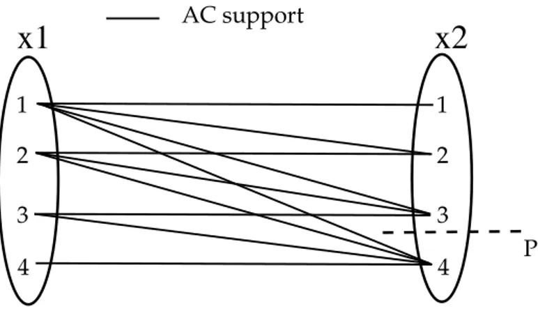
every constraint. By definition, a value(xi, vi)is consistent with a constraintcif and only if it has an AC-support onc, i.e. a combination of values of all variablesvar(c)that satisfy

con whichxitakes the valuevi. A large number of domain-based consistencies stronger than AC have been proposed. Stronger means that they can detect more local inconsis-tencies. These strong domain-based consistencies [Bessiere, 2006] can be divided into Triangle-Based consistencies, Singleton-Based consistencies and inverse consistencies.

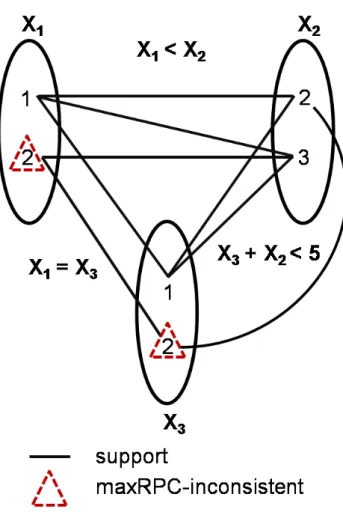
Triangle-Based consistencies deal with triangles. A triangle is a triple of variables

con-nected two-by-two by binary constraints. In other words, triangle-based consistencies deal with triples(xi, xj, xk)withcij ,cjkandcikall inC. In 1995, Berlandier proposes the first Triangle-Based consistency, called Restricted Path Consistency (RPC). In addition to arc consistency, RPC [Berlandier, 1995] guarantees for every value(xi, vi)having only one AC-support((xi, vi), (xj, vj))on a binary constraintcij that the tuple((xi, vi), (xj, vj))can be extend to any third variablexkin a consistent way such that the triple(xi, xj, xk)is a trian-gle. In [Freuder and Elfe, 1996], Freuder and Elfe proposed Path inverse consistency (PIC). PIC is stronger than Restricted Path Consistency, it guarantees for every value(xi, vi)and for every triple(xi, xj, xk)that there exist a value(xj, vj)and a value(xk, vk)such that the tuple((xi, vi), (xj, vj), (xk, vk))is locally consistent. Debruyne and Bessiere generalized re-stricted path consistency to k-consistency max Rere-stricted Path Consistency (maxRPC) [De-bruyne and Bessiere, 1997]. maxRPC is stronger than RPC and NIC. Given a value(xi, vi) and a constraintcij, maxRPC ensures that(xi, vi)has an AC-support((xi, vi), (xj, vj))oncij that can be extend to any third variablexkin a consistent way such that the triple(xi, xj, xk) is a triangle.

Singleton-based consistencies apply the singleton test principle, which consists in

as-signing a value to a variable and trying to refute it by enforcing a given level of consistency. If a contradiction occurs during this singleton test, the value is removed from its domain. Singleton-based consistencies have been shown extremely efficient to solve some classes of hard problems [Bessiere et al., 2011]. Singleton Arc Consistency (SAC) [Debruyne and Bessière, 1997] is the first example of Singleton-based consistency. In SAC, the singleton test enforces arc consistency. Several extensions of SAC have been proposed. Bennaceur and Affane proposed Partition-One-AC (that we call POAC), a Singleton-based consistency stronger than SAC, that can prune values everywhere in the network as soon as a variable has been completely singleton tested. In [Bennaceur and Affane, 2001], the pruning capa-bilities of SAC and POAC was compared. But no algorithm enforcing POAC was proposed. The first algorithm achieving POAC will be presented in chapter 4.

The consistencies stronger than AC that are not domain-based (like k-consistency), op-erate by identifying combinations of values to subsets ofX that cannot be extended to some additional variables. In [Freuder and Elfe, 1996], Freuder and Elfe proposed inverse

consistency principle, a way to enforce forms of local consistencies operating by

identify-ing locally inconsistent combinations of values to subsets ofXwhereas modifying only the domains. Given a subset of variablesS⊆X, inverse consistencies operate by removing val-ues for variables that are inconsistent with all the locally consistent instantiations of the

variables inS. The first local consistency using this principle is the k-inverse consistency [Freuder and Elfe, 1996]. It ensures that any locally consistent instantiation of size1can be consistently extended to anyk − 1additional variables. In other words, for every value

(xi, vi)and for each subsetS⊆Xofkvariables such thatxi∈S, k-inverse consistency en-sures that there exist a locally consistent instantiation of all the variables inSon whichxi takes the valuevi. Focusing on the neighbourhood of a variable, Freuder and Elfe proposed

Neighbourhood inverse consistencies (NIC) [Freuder and Elfe, 1996]. NIC ensures that every

valueviin a domainD(xi)can be extended consistently to all the neighbours ofxi.

Despite the strong consistencies can remove more inconsistent values than AC they re-mains untapped in practice because of the high time complexity of the algorithms enforc-ing these consistencies on a constraint network. In this thesis we focus on the use of con-sistencies stronger than AC to improve the solving efficiency. Before presenting how these higher level local consistencies can be exploited to improve the performance of solvers, we first describe arc consistency and some of these higher level local consistencies. Namely, maxRPC, SAC and POAC.

1.5 arc consistency (AC)

Arc consistency, introduced by [Mackworth, 1977], is the most well known and the most used local consistency in the practice by constraint solvers. It ensures that each value of each variable is consistent with each constraint taken independently. In other words, Arc consistency ensures that each valueviof each variablexi and for each constraintci∈C taken independently, there is at least one combination of values that can be taken by the variables involved inCsimultaneously and where the variablexitakes the valuevi.

1.5.1 Definition

Before giving a formal definition of the of arc consistency property, we first give the definition of a valid tuple then the definition of an AC-support.

Definition 1.10 (Valid tuple) A tuplet∈sol(c_k)_{is valid if and only if ∀}x_i∈var(c_k),t[x_i]∈

D(xi), wheret[xi]is the value thatxitakes int.

Definition 1.11 (AC-support) A tuple t∈sol(ck) is called an AC-support forvi∈D(xi),

xi∈var(ck), onckif and only iftis valid andt[xi] = vi.

For a binary constraintcijsaying thatvj∈D(xj)is an AC-support forvi∈D(xi)oncij is equivalent to say that the tuplet = (vi, vj)is an AC-support forvi∈D(xi)oncij.

Definition 1.12 (Arc consistency) A valuevi∈D(xi)is arc consistent if and only if for each

1.5. ARC CONSISTENCY (AC) 35

vihas no AC-support,viis said to be arc inconsistent. A variablexiis arc consistent if and

only ifD(xi)6=; and all values inD(xi)are arc consistent. A network is arc consistent if all

its variables are arc consistent.

Figure 1.4: Example of Arc-inconsistent values.

Example 1 Let consider the constraintcinvolving two variablesx1and x2 (c≡x1<x2),

with the respective domainsD(x1) = D(x2) ={1,2,3}(Figure 1.4). D(x1)(resp. D(x2)) is

not arc consistent because the value 3∈D(x₁) (resp. 1∈D(x₂)) is inconsistent with the constraintc. Enforcing arc consistency on this constraint will lead to removing the value3

fromD(x1)and removing the value1fromD(x2).

We introduce the notationAC(N)that represents the network obtained by achieving arc consistency on the constraint networkN, i.e. removing every value arc inconsistent in

N. IfAC(N)has an empty domain, we say thatNis arc inconsistent.

1.5.2 AC algorithms

Arc consistency is the most known and most used local consistency in the constraint solvers. Several algorithms have been proposed for establishing arc consistency in a con-straint network. These algorithms can be classified into two categories, fine-grained and

coarse-grained algorithms. In fine-grained algorithms, like AC4 [Mohr and Henderson,

1986], AC6 [Bessière and Cordier, 1993; Bessière, 1994] and AC7 [Bessière and Régin, 1994, 1995], the propagation is value-oriented. If a value(x_i, v_i) has been removed, the fine-grained algorithms check arc consistency for all the values(xk, vk)that had(xi, vi)as AC-support. While coarse-grained algorithms, like AC3 [Mackworth, 1977] and AC2001/AC3.1

[Bessière and Régin, 2001; Zhang and Yap, 2001; Bessiere et al., 2005], are arc-oriented. If the domain of a variablexichanges (i.e., at least a value(xi, vi)has been removed), coarse-grained algorithms check arc consistency for all the other variablesxjsharing a constraint

cwithxi, i.e. arcs(xj, c).

The basic arc consistency algorithm is a brute force algorithm known as AC1 [Mack-worth, 1977]. AC1 is a coarse-grained AC algorithm that simply checks all the arcs repeat-edly until a fixed point of no further domain reductions is reached. In [Waltz, 1975] Waltz realized that a more intelligent arc consistency don’t need to check all the arcs after each domain reduction. It would only rechecks those arcs that could have become inconsistent as a direct result of deletions from a domain. Based on the Waltz’s paper [Waltz, 1975], a more intelligent coarse-grained AC algorithm was proposed known as AC2 [Mackworth, 1977]. The AC2 propagates the revisions of the domains through the arcs until, again, a fixed point is reached. AC3, presented by Mackworth [Mackworth, 1977], is a generaliza-tion and simplificageneraliza-tion of AC2. AC3 is the simplest and the most well-known algorithm for enforcing arc consistency in a constraint network. However, the time complexity of AC3 is not optimal. It achieves arc consistency on binary networks inO(ed3)time andO(e)

space.

The first AC algorithm with an optimal worst-case time complexity is AC4 [Mohr and Henderson, 1986]. AC4 is also the first fine-grained AC algorithm. It uses the data struc-turecounterxi,vi,xj for counting for each value(xi, vi)the number of AC-supports it has

on each constraintcij and uses listsSxi,vi storing all values that are supported by(xi, vi)

on a constraint. AC4 achieves arc consistency on binary networks in O(ed2) time and

O(ed2)space. Although AC4 has an optimal worst case time complexity, Wallace showed in [Wallace, 1993] that AC4 is almost always slower than AC3. This is due to the bad av-erage time complexity of AC4. To improve AC4, Bessière and Cordier proposed AC6 that reduces memory complexity and improves the average time complexity. In opposite to AC4, the idea in AC6 is not to count all the supports a value has on a constraint, but just to ensure that it has at least one. Hence, it only need lists Sxi,vi storing values currently

having(xi, vi)as smallest AC-support. AC6 is a fine-grained AC algorithm achieving arc consistency on binary networks inO(ed2)time andO(ed) space. AC6 has been further improved to AC7 [Bessière and Régin, 1994] which exploits the notion of bidirectionality, i.e. if a support (vi, vj)is found for vi∈D(xi) on the constraintcij, when looking for a support forv_i∈D(x_i), then(v_i, v_j)is also a support forv_j∈D(x_j)onc_ij.

In 2001, the first optimal coarse-grained AC algorithm have been independently pro-posed, namely AC2001 [Bessière and Régin, 2001] and AC3.1 [Zhang and Yap, 2001]. AC2001/3.1 achieves optimality by storing the smallest AC-support for each value(x_i, v_i)

on each constraint cij. Indeed, when a support of a value (xi, vi) has to be found, AC3 starts the search from scratch whereas AC2001/3.1 starts the search from a resumption point which corresponds to the last AC-support found for this value and stored in the data structureLastACxi,vi,xj. This algorithm achieves arc consistency on binary networks in

1.5. ARC CONSISTENCY (AC) 37

O(ed2)time andO(ed)space. Using the notion of bidirectionality, AC2001/3.1 algorithm has been further improved to AC3.2 and AC3.3 in [Lecoutre et al., 2003].

In the following, we give a short description of the more known AC algorithm, namely AC3. Then, we present a more detailed description of AC2001/3.1 [Bessière and Régin, 2001; Zhang and Yap, 2001; Bessiere et al., 2005], the optimal coarse-grained AC algorithm.

AC3 Algorithm

The AC3 algorithm is a coarse-grained algorithm that was proposed in [Mackworth, 1975] for binary normalized networks and extended to GAC for arbitrary networks in [Mackworth, 1977]. The AC3 Algorithm consists to guarantee for each pair(xi, c)(arc) that the values in the domain ofxiare arc consistent onc. This Algorithm uses a propagation queue in order to hold all the arcs(xi, c)that need to be revised. Initially, all the possible arcs(xi, c)such thatxi∈var(c)are put in the propagation queue. Then, arcs(xi, c)are revised in turn, to remove the values ofD(xi)that have become inconsistent with respect toc. When a revision is effective (i.e., at least a value has been removed), the propaga-tion queue is updated by adding all pairs,(xj, c0)such thatxi6= xj andxi, xj∈var(c0), for which we are no longer guaranteed thatD(xj)is arc consistent onc0. In fact, the deletion of a valuevi∈D(xi)can induce as a side effect the deletion of other valuesvj∈D(xj), which were previously recognized as arc consistent on a constraintc0such thatxi, xj∈var(c0). The algorithm stops when a domain becomes empty as we are guaranteed that the prob-lem is unsatisfiable or when the propagation queue is empty as we are guaranteed that all arcs have been revised and all remaining values of all variables are consistent with all constraints. AC2001 Algorithm Algorithm 2: AC2001(X, D, C) 1 begin 2 Q← {(x_i, c_ij)|c_ij∈C∧x_i∈scop(c_ij)}; 3 whileQ6=; do

4 select and delete(x_i, c_ij)fromQ 5 ifRevise(x_i, c_ij)then 6 ifD(xi) =; then 7 returnfalse; 8 else 9 Q← Q∪{(xj, cik)|cik∈C∧cik6= cij∧scop(cik) ={xi, xk}}; 10 returntrue;

Algorithm 3: Revise (xi, cij)

1 begin

2 CHANGE← false 3 foreachv_i∈D(x_i)do

4 ifLastAC_xi,vi,xj∉D(x_j)then

5 if¬SeekSupport(x_i, v_i, x_j,LastACxi,vi,xj)then

6 removev_ifromD(x_i) 7 CHANGE← true 8 returnCHANGE

Algorithm 4: SeekSupport (xi, vi, xj,LastACxi,vi,xj)

1 begin 2 foreachv_j∈D(x_j), v_j>LastACxi,vi,xjdo 3 if(v_i, v_j)∈c_ijthen 4 LastACxi,vi,xj← vj 5 returntrue 6 returnfalse

AC2001/AC3.1 [Bessière and Régin, 2001; Zhang and Yap, 2001; Bessiere et al., 2005] is the first worst case optimal coarse-grained algorithm enforcing arc consistency in a con-straint network. To be optimal, the AC2001/AC3.1 algorithm stores the support of each valuev_i∈D(x_i)on each constraintc_ijusing the structureLastACxi,vi,xj. Indeed,

when-ever an arc(xi, cij)is revised, AC3 starts the search of support for each valueviin the do-main ofxifrom scratch whereas AC2001/3.1 starts the search of a support for a valuevi, from the last support found for this value and stored in the structureLastACxi,vi,xj, only

if the valuevj(support) stored inLastACxi,vi,xjis no longer inD(xj).

The pseudo-code of the AC2001/3.1 algorithm is presented in algorithm 2. Initially, all arcs(x_i, c_ij)are inserted in Q (line 2). Then, iteratively, each arc of Q is revised (line 3). A revision of an arc(xi, cij)is performed by a call to the functionRevise(xi, cij)and aims at removing the valuesvi∈D(xi)that are arc inconsistent oncij. When the revision of an arc

(x_i, c_ij)is effective (at least a value has been removed), two cases are possible. IfD(x_i)is wiped out, the algorithm returns false (line 7). Otherwise, all the arcs(xk, cik)withi6= kare added to Q (line 9). The algorithm is stopped when the queue Q becomes empty (line 10) or when a domain is wiped out (line 7).

The functionRevise(xi, cij), depicted in algorithm 3, checks for each valuevi∈D(xi) if it is still consistent on the constraintcij. It checks first if the support, founded in a