EVALUATION OF PHASE-TO-PHASE CLEARANCES OF TRANSMISSION LINE CONDUCTORS UNDER TURBULENT WIND
Louis-Philippe Parent, Sébastien Langlois, Kahina Sad Saoud Université de Sherbrooke - Canada
Introduction
Wind loads govern the design of a large number of overhead transmission lines worldwide. The spatial and temporal variation of wind speed and the buffeting response of cables may induce swings not fully synchronized between two parallel cables, thus raising serious concerns regarding phase-to-phase clearances. Accurate assessment of the minimum mid-span clearances to be considered in the design of transmission lines is essential to avoid repetitive flashover episodes and hence ensure the reliability of the electrical system. In practice, a wide range of empirical formulae is proposed to evaluate the critical phase-to-phase clearance distances for various transmission line configurations. For instance, the European standard CENELEC EN-50341 [1] provides a simple equation for the minimum horizontal spacing in the case of standard line heights not exceeding 60 m [2]. However, such formulae do not consider all the geometric and wind parameters affecting the phase-to-phase clearances, which is of key importance for efficient and economic design.
This paper seeks at studying the most influential parameters affecting the phase-to-phase clearances in extreme wind events. A time-history numerical model is specifically developed using the finite element open software Code_Aster, where the behavior of both the conductors and insulator strings is represented using one-dimensional elements accounting for large displacements. The applied turbulent wind signals are also generated numerically, as functions of time and space coordinates. A two-span transmission line section including two phase conductors is considered herein to carry out a parametric study for various geometric and wind conditions. The results reveal that an empirical formula, considering only the conductor sag and insulator length, often yields misleading results.
NUMERICAL MODELING PROCEDURE
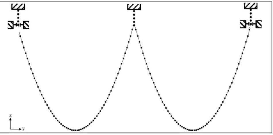
The present study is devoted to the numerical modeling of the dynamic response of a two-phase transmission line subjected to gusty wind conditions. We consider a line section comprising single bare conductors attached to suspension insulator strings, themselves clung to the support structures that are not covered in this work for the sake of simplicity. The numerical modeling is performed using the finite element package Code_Aster, where both the conductors and insulators are modeled as flexible wires undergoing large displacements and rotations by means of CABLE elements. The materials constituting the conductors and insulators are assumed to be isotropic and homogeneous with a linear elastic constitutive law. As illustrated in Figure 1, the motion of each insulator string is restricted at its end attached to the support structure, the other end being simply attached to the cables except for the insulators located at both extremities of the transmission line section where no displacement along y-axis is allowed.
The numerical study comprises two main stages: a non-linear static analysis and a non-linear transient dynamic analysis. On the one hand, the static analysis, in which the studied structure is subjected only to a vertical loading due to its self-weight, enables the initial sagging of the conductors as catenaries. A dummy temperature variation is applied on the conductors so that the horizontal component of tension approximately equals the nominal tension of 20 % RTS and is almost the same within all the
spans, for all the cases handled in this paper. On the other hand, the transient dynamic problem, derived in the updated Lagrangian framework, leads to the following global system of equations:
( )
Mu Cu Ku
f t
(1) where M, C and K stand for the global mass, damping and stiffness matrices, respectively. u is the global nodal displacement vector,u
andu
are its first and second time derivatives, respectively. Finally, f designates the vector of external wind loads.
Figure 1. Numerical representation of two adjacent spans with boundary conditions
The time-dependent wind load acting on a given node P of the analyzed structure may be split into two parts, as follows [3]:
( , )
( )
t( , )
C P t
F P
f P t
(2) The mean wind loadF
, depending on the mean wind velocityV
, may be expressed by the following:2
1
( )
( )
2
air dF P
C A V P
(3)The turbulent part of the wind load
f
t may take the following form:( , )
( )
( , )
t air d
f P t
C A V P
u P t
(4) wherein
airstands for the air density, andA
represents the exposed area of the conductors (A
is equal to the conductor diameter times the wind span). In the present study, the drag coefficient of the conductorsC
d is calculated as a function of the average wind speed from an empirical formula by Prud’homme [4]. The mean wind velocityV
is defined as a function of height above groundz
by the following logarithmic formula [3]:* 0
( )
2.5 ln
z
V P
u
z
(5)where
u
* is the wind shear velocity andz
0the roughness length. The turbulent wind velocityu
is generated numerically using an in-house program called WindGen [5], which relies on the spectralrepresentation algorithm by Shinozuka and Deodaties [6] to simulate the space and time correlated signals.
It is worth mentioning that, in the numerical model, the wind load is applied only on the cables, as a time-dependent loading, and no wind is applied directly on the insulator strings. Rayleigh damping is applied throughout this study, with damping ratios of 0.1 % and 20 % affected to the cables and insulators, respectively, based on a preliminary numerical study. A direct time integration is performed using the implicit Newmark scheme with β = 0.25 and γ = 0.5, and the whole problem is solved in an incremental way using the classical Newton-Raphson method so as to encompass the geometric non-linearities due to conductor motions.
Subsequently, a test case related to an experimental line [7] is reproduced numerically; the results are set against the experimental data provided by Hydro-Québec, so as to assess the accuracy of the present numerical procedure. Once validated, the numerical model is used to carry out a parametric study to evaluate the effect of various geometric and wind parameters on the phase-to-phase clearances. The analyzed parameters include: phase-to-phase spacing at rest, conductor span and sag, average wind speed, and turbulence intensity of the wind. For each of these parameters, the numerical clearances are compared with results from an empirical formula by Kiessling [2].
VALIDATION OF THE MODEL AND DISCUSSION
The numerical procedure described above is employed here to study a three-span line section, for which experimental results are available for comparison [7]. The equivalent material characteristics of the considered Bersfort conductors and insulator strings are summarized in TABLE 1, where E stands for the Young’s modulus, ν the Poisson’s ratio, and ρ the mass density.
E (MPa) ν ρ (kg/m3) ACSR Bersfort cables 6.76x10⁴ 0.3 2380
Insulators 2.00x10⁵ 0.3 63232
TABLE 1 – Material properties of the conductors and insulators
As regards geometry, the conductors are attached to insulator strings of 3.4 m length. The attachment point concerning the first tower is located at 24.84 m above ground. The relative positions of the remaining attachment points are indicated in TABLE 2.
Span 1 Span 2 Span 3
Horizontal separation (m) 274 366 457
Vertical separation (m) 0 1.25 0
TABLE 2 – Geometric characteristics of the considered line section
The finite element discretization employs 10 fully integrated first-order (linear) elements within each insulator string. For the conductors, use is made of 30 fully integrated first-order elements along the span 1, and 40 elements along each of the spans 2 and 3.
The applied wind loading is generated to conform as much as possible to the wind spectrum obtained at the Magdalen Islands, where the reference tests were carried out during the period of winter 1989-1990. The mean wind speed at 10 m, assumed to be constant along the line span, is computed over 5 minutes based on measurements recorded at several locations on the experimental line. Nine examples, where the wind acts perpendicular to the test line, are particularly retained for the validation procedure. This simplifies the generation of the numerical wind. Let us mention that the dynamic
analysis is performed separately for each of the two phase conductors, however, that is not supposed to affect the validity of the results since the wind signals are generated for the whole structure, taking into account the geometric correlation.
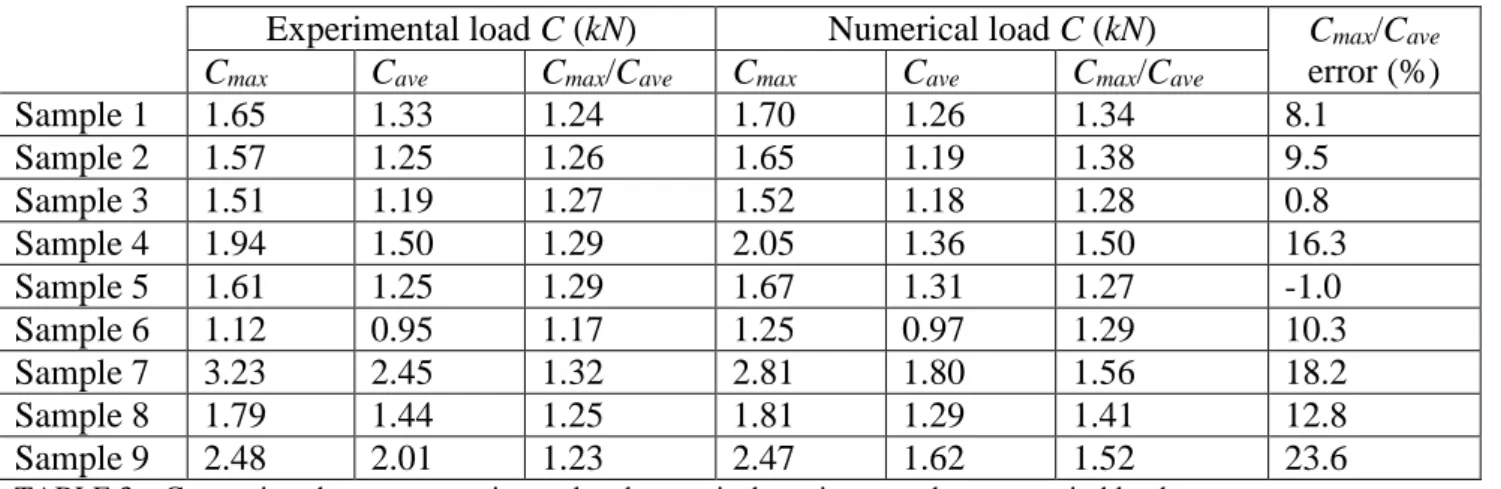
In the numerical model, five wind signals are generated for each of the nine test samples considered; the experimental and numerical wind loads are reported in TABLE 3. One may readily notice that the wind conditions at Magdalen Islands are not always easy to reproduce numerically for numerous reasons that will not be featured here as it goes beyond the scope of this paper. The comparison between the ratios of maximum load Cmax and average load Cave shows that WindGen provides results
close to the experimental ones for only samples 3 and 5.
Experimental load C (kN) Numerical load C (kN) Cmax/Cave
error (%) Cmax Cave Cmax/Cave Cmax Cave Cmax/Cave
Sample 1 1.65 1.33 1.24 1.70 1.26 1.34 8.1 Sample 2 1.57 1.25 1.26 1.65 1.19 1.38 9.5 Sample 3 1.51 1.19 1.27 1.52 1.18 1.28 0.8 Sample 4 1.94 1.50 1.29 2.05 1.36 1.50 16.3 Sample 5 1.61 1.25 1.29 1.67 1.31 1.27 -1.0 Sample 6 1.12 0.95 1.17 1.25 0.97 1.29 10.3 Sample 7 3.23 2.45 1.32 2.81 1.80 1.56 18.2 Sample 8 1.79 1.44 1.25 1.81 1.29 1.41 12.8 Sample 9 2.48 2.01 1.23 2.47 1.62 1.52 23.6
TABLE 3 – Comparison between experimental and numerical maximum and average wind loads
The resulting numerical reaction forces and swing angles of the second insulator string θ, which may be obtained from equation (6), are now compared with the corresponding experimental results.
2 2 1
sin
isox
z
L
(6)where Δx and Δz designate the displacements in the x-direction and the z-direction, respectively, and Liso represents the insulator string length. The numerical modeling using Code_Aster properly
simulates the response of samples 3 and 5, since the numerical winds comply with the experimental ones. Moreover, the experimental and numerical results show similar trends for the remaining samples, although the numerical winds are not properly simulated. For example, it is noted that the swing angles become larger when the wind load intensities increase, as indicated in TABLE 4.
Experimental angle θ (°) Numerical angle θ (°) θ max θ ave θ max θ ave
Sample 1 10.16 8.32 10.33 7.69 Sample 2 9.59 7.74 10.04 7.26 Sample 3 9.10 7.34 9.24 7.21 Sample 4 11.79 9.30 12.41 8.30 Sample 5 9.76 7.80 10.15 7.98 Sample 6 6.87 5.95 7.64 5.93 Sample 7 18.44 14.88 16.96 10.88 Sample 8 10.92 8.88 11.02 7.84 Sample 9 14.81 12.34 14.91 9.83
PARAMETRIC STUDY
A series of calculations are carried out in the following using the developed numerical model for different combinations of geometric and wind parameters. This should provide a scientific basis for equations in the literature used by engineers. Among many other formulae, the following one, defining the minimum clearance required between two phase conductors at mid-span [2], is considered in this study:
min c c k
0.75
ppd
k
f
l
D
(7) In equation (7), onlyk
cf
c
l
k , representing the loss of clearance due to wind, will be considered; where kc designates a coefficient depending on the relative position between the conductors, fcrepresents the conductor sag at a temperature of 40 °C, and lk is the length of the insulator part that
may swing perpendicular to the line direction.
A line section of two identical level spans is now considered to perform the parametric analysis (see Figure 1 for the definition of the boundary conditions). The material properties of the conductors and insulator strings are those given in TABLE 1. The model mesh uses fully-integrated linear elements with a length of approximately 4.3 m. The dynamic analysis is achieved using Code_Aster over a time period of six minutes, including a one minute ramp at the beginning of the analysis to stabilize the wind forces. Let us define the reference case with the following parameters: phase-to-phase spacing at rest (10 m), span length (275 m), conductor sag (7.973 m), average wind speed at 10 m (15 m/s), turbulence intensity (25 %). The spatial correlation of the wind takes up the parameters defined in [8]. In the sequel, the maximum loss of clearance between the same nodes of two parallel conductors will be determined for each of the previous set of parameters. For each pair of nodes, a loss of clearance is evaluated by taking the initial phase-to-phase spacing and subtracting the minimum distance recorded during the time response. The distance d is calculated using the following equation:
2 2 2
d
x
y
z
(8) in which Δy designates the displacement in the y-direction.Then, only the maximum loss of clearance for the line section is retained for a given analysis. As for the validation tests, five numerical wind signals are generated for each of the studied set of parameters, the results presented subsequently are the average values.
Parameter 1: Phase-to-phase spacing at rest
The following values are considered for the initial separation between phases: 6 m, 8 m, 10 m, 12 m, and 14 m. All the other parameters are those defined for the reference case. The results of the dynamic analysis are depicted in Figure 2. The numerical results show that the initial phase-to-phase spacing does not affect the maximum loss of clearance, which is in agreement with the equation of Kiessling. Moreover, the two models give close results for the maximum loss of clearance.
Parameter 2: Span length
Spans of 275 m, 350 m, and 425 m are considered here, which corresponds to sags of 8.62 m, 12.68 m, and 17.58 m, respectively. The remaining parameters are those of the reference case, particularly the mechanical tension is set at a constant value. The corresponding results are reported in Figure 3. One may readily notice that both models agree that the loss of clearance increases as the span length
increases. However, the results from the numerical model are higher than those predicted by the theoretical model for the spans of 350 m and 425 m. Notice that the loss of clearance values for parameter 2 are not affected by only the span length, since the sag varies accordingly. Further studies are hence required to isolate the effect of the span length.
Figure 2. Maximum loss of clearance for various phase-to-phase spacing at rest
Figure 3. Maximum loss of clearance for various span lengths
Parameter 3: Conductor sag
The conductor sag is controlled here by adjusting the mechanical tension level, defined as a percentage of the rated tensile strength (RTS). Tensions of 15 %, 20 %, and 25 % of RTS are considered, giving sags of 10.12 m, 8.62 m, and 7.86 m, respectively. Results are shown in Figure 4.
As one may expect, the initial sag influences the loss of clearance of conductors. For a tension of 15 % of RTS, the two models are in a good agreement, with only 4 % of relative error. For the other considered values, the equation of Kiessling overestimates the maximum loss of clearance.
Parameter 4: Average wind speed
The average wind speed is mainly controlled by the wind shear velocity
u
* and the roughness length 0z
. However, the wind velocity is controlled here by only modifying the wind shear velocity, as the turbulence intensity, which depends on coefficientz
0, must stay constant here. The following velocities are considered: 10 m/s, 12.5 m/s, 15 m/s, 20 m/s, and 25 m/s. The associated results are presented in Figure 5. From the numerical results, one may notice that, unlike the predictions given by the equation of Kiessling, the wind speed has an important effect on the clearances. The maximum relative error between the two models reaches 130 % (for 25 m/s). It should be mentioned that this equation is not meant to be applicable for high wind speeds, for which ultimate limit state load cases are considered rather than phase spacing criteria.
Figure 5. Maximum loss of clearance for various average wind speed
Parameter 5: Turbulence intensity
The following values are taken for the turbulence intensity: 15 %, 20 %, 25 %, 30 %, and 35 %. Results of the parametric analysis are summarized in Figure 6. Unlike the results from the equation of Kiessling that neglects the effect of the turbulence intensity, the numerical results provide an increase of the maximum loss of clearance with the increase of the turbulence intensity.
CONCLUDING REMARKS
This paper deals with the numerical modeling of a two-phase conductor subjected to turbulent wind conditions. A numerical model using the finite element software Code_Aster is developed so as to study the transient dynamic response of a line section subjected to gusty winds. The applied load is also generated numerically, by means of a specific program WindGen. The results from the proposed model were first compared with experimental results. It has been shown that the numerical model gives accurate results, as long as the numerical wind signals are properly generated. A parametric analysis was carried out for various geometric and wind conditions. Unlike the equation of Kiessling, which considers only the conductor sag and the length of the insulator strings, the numerical results have shown that the phase-to-phase clearances are particularly influenced by the conductor span/sag, the average wind velocity, and the turbulence intensity.
From the previous parametric study, a simple and accurate method for the evaluation of the phase-to-phase clearances may be proposed for future research. Further analysis, for example, involving larger line sections, other wind signal parameters, and different line configurations, are also required.
REFERENCES
[1] CENELEC EN-50341, 2012, Overhead electrical lines exceeding AC 45 kV, European Committee for Electrotechnical Standardization.
[2] F. Kiessling, P. Nefzger, J. Nolasco and U. Kaintzyk, 2003, Overhead Power Lines: Planning, Design, Construction, Springer, Berlin, Germany.
[3] E. Simiu and R. Scanlan, 1996, Wind effects on structures: fundamentals and applications to design, John Wiley & Sons Inc., New York, USA.
[4] S. Prud’homme, 2010, Développement d’un banc d’essai actif et passif à 3 DDL pour essais sectionnels en soufflerie, Université de Sherbrooke, Canada.
[5] S. Hang, F. Gani and F. Légeron, 2005, Générateur de vent appliqué au Génie Civil : WindGen, Université de Sherbrooke, Canada.
[6] M. Shinozuka and G. Deodatis, 1991, "Simulation of stochastic processes by spectral representation", Applied Mechanics Review, vol. 44, 191-204.
[7] S. Houle, 1990, Chargement statique et dynamique des pylônes de lignes de transport causé par la pression du vent sur les conducteurs : mesures dans des conditions réelles d’exposition au vent - Rapport No 08-Q-399, Hydro-Québec, Îles-de-la-Madeleine, Canada.
[8] G. Solari and G. Piccardo, 2001, "Probabilistic 3-d turbulence modeling for gust buffeting of structures", Probabilistic Engineering Mechanics, vol. 16, 73-86.
Acknowledgements
The National Sciences and Engineering Research Council of Canada (NSERC), funding program InnovÉÉ, RTE and Hydro-Québec are gratefully acknowledged for their financial support.