High-frequency monitoring of surface water quality at the outlet of the Ibrahim River (Lebanon): A multivariate assessment

OATAO is an open access repository that collects the work of Toulouse

researchers and makes it freely available over the web where possible

Any correspondence concerning this service should be sent

to the repository administrator:

tech-oatao@listes-diff.inp-toulouse.fr

This is an author’s version published in:

http://oatao.univ-toulouse.fr/24568

To cite this version:

El Najjar, Paula and Kassouf, Amine and Probst, Anne

and Probst, Jean-Luc

and

Ouaini, Naim and Daou, Claude and El Azzi, Désirée High-frequency monitoring of

surface water quality at the outlet of the Ibrahim River (Lebanon): A multivariate

assessment. (2019) Ecological Indicators, 104. 13-23. ISSN 1470-160X

High-frequency monitoring of surface water quality at the outlet of the

Ibrahim River (Lebanon): A multivariate assessment

Paula El Najjara, Amine Kassou

f">

, Anne Probst

C

_,

_{Jean-Luc Probst}

C

_{, Naim Ouaini\ Claude Daou\}

Desiree El Azzi

a

_,

_*

•

Faculry of A8rlcultural and Food Sciences, Holy Spirit University, Kasllk, Jounieh B.P. 446, Lebanon

"Depanment of Chemisa-y and Bwchemt.say, Faculty of Sciences n, Lebanese University, 90656 Fanar, Jdeldedt El Mam, Lebanon 'EcoLab, Untverslre de Toulouse, CNRS, UPS, INPT, Campus ENSAT, Avenue de l'Agroblopole, 31326 Casronet Tolosan CEDEX, France ARTICLE I NFO

Keywords:

Surface water monltorlng Prlndpal COmponent Analysls

Parameters' reductlon Lebanon

Water quallty Index

1. Introduction

ABSTR A CT

Surface 11vater quality monitoring is essential to evaluate the quality of a water resource. The current study assesses the quality of the Ibrahim River, one of the main Lebanese rivers, exposed to considerable human activities. 285 samples were collected at the outlet of the river, between May 2016 and July 2017, covering one hydrological year. Twenty-three physico-chemical parameters (flow, pH, temperature, electrical oonductivity, turbidity, total suspended solids, total dissolved solids, dissolved oxygen, dissolved organic carbon, biochernical oxygen dernand, chemical oxygen demand, chemical oxygen dernand/biochernical oxygen dernand, specific ultraviolet absorbance, dissolved cations (Na+_{, K +, Ca}2+_{, Mg}2+ _{), total alkalinity, dissolved anions (Cl-, NO}

3 -, NO2 -, Po,3- and so.2-)) and five microbiological tests were assessed (total germs, total ooliforms, fecal co­ liforms, Escherichia coli and Enterococcus). A Principal Component Analysis (PCA) was applied for data analysis. The first component showed high levels of anthropogenic characteristics mainly due to organic and b.�cter­

iological parameters, differentiating low and high river discharges (explaining around 35% of the total var­ iance). The second component was mainly influenced by minerai variables showing a clear annual dis­ crimination (explaining about 17% of the total variance). Moreover, this study led to variables reduction from twenty-eight to ten. The final shortlisted parameters are Q, pH, EC, NO3 -, total coliforms, fecal coliforms, B0D5, K+_{, TA and ci-. A new PCA performed with the reduced matrix validated this selection. The water quality index} (WQI) was then calculated in this study, using the shortlisted parameters characteri2ing the basin, excluding the flow since it cannot be considered as a quality indicator. Thus, the 11vater was evaluated as« medium» to « good » 111,ith values ranging from 63.1 (August 2016) to 73.1 (Novernber and Decernber 2016) with an average of 69.0 ± 1.9. The proposed WQI should be further tested for monitoring practices in the Ibrahim River basin or other similar b.�ins of the region.

Surface water is vulnerable to pollution from anthropogenic activ­ ities, mainly waste disposai and agricultural practices. Due to the ac­ cumulation and transport of pollutants, rivers are important vectors of pollution. With about 40 rivers, Lebanon is rich in surface and ground water as compared to neighboring countries of the Middle East and North Africa region (Assaf and Saadeh, 2008; Chamas et al., 2001). Despite this water richness, water availability and quality are sig­ nificantly declining due to the Jack of efficient management plans and the widespread pollution sources. Pollution mostly results from the growing population, the industrial development, the agricultural

activities, the uncontrolled discharges of industries and the solid waste rnismanagement (Abu-Jawdeh et al., 2000; El-Fadel et al., 2000; Singh et al., 2004, SOER, 2001). Severa! studies on Lebanese rivers showed that their water quality has deteriorated due to many human activities (Assaf and Saadeh, 2008; Houri and El Jeblawi, 2007; Kabbara et al., 2008; Massoud, 2012). In addition, climate change and global warming are Jeading to significant disturbances of hydrological cycles and thus, are affecting water pollution (Fan et al., 2010, Giannakopoulos et al., 2009). Ail these problems have a direct impact on the functioning of ecosystems and biodiversity.

As rivers are the source of water used for most inland human ac­ tivities, it is important to constantly control their quality taking into

• Corresponding author.

E-mail address: desireeelazzi@usek.edu.Jb (D. El A2zi).

2.2. Sampling and pretreatment

From May 2016 to July 2017, water samples were collected at a predefined sampling station located at the Ibrahim River outlet (long-itude is 34° 3742 N and the lat(long-itude is 35° 38,724E). This station collects all the water drained by the river as well as all the materials transported to the sea (Fig. 2). It should be noted here that frequent measurements of water salinity were carried out at the beginning of the work, to locate the appropriate study site avoiding the mixing zone between freshwater and seawater. An automatic sampling device, equipped with a pump, was installed at the study site. Samples were then collected mechani-cally from the middle of the river, at an equal distance from the two shores (Hébert and Légaré, 2000).

Water was collected by an aspiration pump via a sterile exchange-able polyethylene pipe that is coated with a grey polypropylene pro-tective tube. The mentioned sampling system pump is equipped with a small modifiable valve in the purpose to regulate the water flow rate required for our sampling. Basic precautions were considered to avoid any pump malfunction, especially during flood events. Thus, the sam-pling device was safely protected in a small shelter placed on a concrete slab.

A hydrometric station operated by the Litani River Authority (LRA) is already installed at this location. As a result, discharge measurements were available. During the entire study period, discharge fluctuated between 0.05 and 60.29 m3_{/s (Flow rate average of 36 ± 13.74 m}3_/s). 95 sampling points are represented on the hydrograph (Fig. 3). One sampling was scheduled per week except during flood events, when samples were collected every two hours.

Prior to water sampling, 1L polypropylene bottles were cleaned with a laboratory grade detergent (phosphate-free) and rinsed with distilled water and nitric acid 10% (Demirak et al., 2006; Rodier et al., 2009). These bottles were used for physico-chemical tests. In parallel, borosilicate amber glass bottles of 1 L capacity were prepared for mi-crobiological tests. They were rinsed with distilled water to remove any detergent traces or residues and then sterilized by autoclaving at 120 °C for 15 min before each sampling.

Each sampling point represented on Fig. 3 corresponds to three polypropylene bottles and three borosilicate amber glass bottles (of 1L capacity each). In total, 285 samples were collected. All bottles were labeled with the sampling date and time, then stored at 4 °C in a por-table refrigerator and directly transported to the laboratory, as re-commended by the French standards organization AFNOR (NF T90-100). Once in the laboratory, all microbiological analysis tests were conducted on the borosilicate bottles within 24 h of the sampling.

Concerning the polypropylene bottles, 700 mL of each poly-propylene bottle was filtered through a cellulose nitrate membrane filter (0.22 μm pore size) previously rinsed with ultrapure water. Half of the filtrates were then stabilized by acidification with few drops of high purity nitric acid. All samples were stored in a cold room at around 4 °C, in complete darkness. An accomplishment of the study within a period of 24 h up to few months after the sampling campaign is still possible, if the water samples are properly stored (Hébert and Légaré, 2000). 2.3. Physico-chemical analysis

Several chemical, physical or biological reactions may occur inside the sampling bottle and can directly affect the composition of the col-lected sample. Since some of these reactions are too fast, there may be a lot of changes and effects in the first few minutes after the collection. Therefore, these countless reactions can influence the concentrations of many elements and may have a vast impact on the tested parameters. Thus, in situ analysis, within 5 min after sampling, are necessary for some of the measured indicators (Ahoussi et al., 2012). The main parameters tested on site were pH, conductivity (µS/cm), temperature (°C), dissolved oxygen (mg/L) and turbidity (NTU). The accuracy of consideration temporal and spatial variations. For efficient monitoring,

many physico-chemical, bacteriological and hydrological parameters should be studied. Such monitoring, if applied on every river in a country, would demand significant financial inputs. Thus, it is of utmost importance to optimize the monitoring activity by reducing the number of tested parameters without losing significant i nformation (Singh et al., 2004). To do so, multivariate approaches such as Principal Component Analysis (PCA) can be used (Fan et al., 2010; Simeonov et al., 2003; Singh et al., 2004). In fact, PCA was largely used to eval-uate the seasonal and particular variations, identify potential sources of pollution (Barakat et al., 2016; Sharma et al., 2015; Simeonov et al., 2003) and reduce the dimensionality of a data set while retaining most of the existing information and variability in the data (Alberto et al., 2001). Once the number of monitored parameters is reduced, water quality indexes (WQI) was calculated providing a single dimensionless number reflecting t he i nfluence of di fferent wat er qua lity parameters (Ramakrishnaiah et al., 2009; Sutadian et al., 2018). It has been used worldwide to evaluate water quality and management effectiveness and is becoming one of the most effective tools of communication to citizens and policy makers (Sutadian et al., 2018).

Therefore, the main objective of this study is to evaluate the water quality of the Ibrahim coastal basin, one of the main Lebanese rivers, classified as World Heritage Site (Fitzpatrick et al., 2001) and propose a reduction of factors to monitor this river without losing information. By linking WQI and PCA methodologies, this work will help upcoming water strategies in Lebanon (Reza and Singh, 2010; Tyagi et al., 2013). Water samples were collected at the outlet of the Ibrahim River with higher density during flood events. In fact, high fluxes of materials are exported to the outlet of rivers during these hydrological events (El Azzi et al., 2013; El Azzi et al., 2016; Taghavi et al., 2011). Both physico-chemical and microbiological parameters were then tested, and a multivariate study formed the basis for the development of an Ibrahim WQI (IWQI) which would reliably describe and rate the quality of the water in the future.

2. Materials and methods

2.1. Study site

The Ibrahim River is 28 km long and estimated as one of the largest rivers in Lebanon (Chamas et al., 2001; Fitzpatrick et al., 2001). It is located 20 km north of the Lebanese capital and has an annual average flow of 16,106 m3_{/year (Abboud, 2002; Chamas et al., 2001). Its source} is located at the top of Mount Lebanon (Roueiss and Afqa) and flows westward discharging through the city of Jbeil, into the Mediterranean Sea (Papazian, 1981).

The Ibrahim watershed has a total area of 330 km2 _{with a structure} consisting mainly of Jurassic and Cretaceous limestones (El Amil and Oudwane, 2000; Papazian, 1981). It presents high flows during winter and autumn seasons, but low flow o ccurs i n l ate s ummer (Fitzpatrick et al., 2001). Two perennial sources Roueiss and Afqa, located respec-tively at an altitude of 1300 and 1200 m, ensure the flow of the river all year through. In addition, other additional tributaries with about thirty different s ources f eed t he m ain r iver (El A mil a nd O udwane, 2000; Papazian, 1981). The industrial activities on the Ibrahim River are mainly referring to small firms s uch a s m arble a nd f ood factories, woodcraft industries and many repair workshops. The agricultural sector consumes the greatest part of water in the basin. It occupies only 7.8% of the basin’s total surface and is largely concentrated at the river mouth. Agricultural fields a re m ainly o ccupied b y f ruit b earing trees, citrus and banana plantation (Fig. 1). The rest of the basin is occupied by non-fertile lands (43%), oak trees and mixed forests (37%) and herbaceous vegetation (10%). Hill dams occupy only 0.42% and are distributed throughout the basin (Assaker, 2016; Daou et al., 2013).

each measurement was ensured by previous calibrations using appro-priate buffer solutions (Lamizana-Diallo, 2008). Table 1 shows the studied parameters and the used analytical methods for each analysis. 2.4. Microbiological analysis

The water microbiological analysis was completed to detect and evaluate the existence of germs (Ouhmidou and Chahlaoui, 2015; Bou Saab et al., 2007; Daou et al., 2018). The presence of total germs (CFU/ 100 mL), total coliforms (CFU/100 mL), fecal coliforms (CFU/100 mL), Escherichia coli (CFU/100 mL) and Enterococcus (CFU/100 mL) was ex-amined (Table 1).

The enumeration of culturable micro-organisms (total germs at 37 °C) was completed by inoculation in a nutrient agar culture medium followed by colony counting (ISO 6222:1999(E)). The used method for total coliforms, fecal coliforms, Escherichia coli and Enterococcus isola-tion is the membrane filtraisola-tion technique by introducing water into a sterilized filtration unit containing a gridded sterile cellulose nitrate membrane filter of 0.45 µm diameter (NL ISO 9308-1:2012 and ISO 7899-2:2000(E)). After applying the vacuum, germs were retained on the filter that was then placed on the appropriate culture medium. Petri dishes were transferred to incubators at suitable temperature for 24–48 h and colonies were counted under a BOECO colony counting equipment. Results are expressed as the number of colony-forming units

per 100 mL (CFU/100 mL) of tested water.

2.5. Chemometric analysis: Principal Component Analysis (PCA) PCA is an unsupervised exploratory method frequently used in surface water quality monitoring, for various purposes among which one could mention: modeling, outlier detection, variable selection and classification. Considering a set of n samples described by p variables, the data is gathered in a matrix X with n rows and p columns. In our case, a row of X corresponds to 28 physicochemical and microbiological measurements obtained from the analysis of a surface water sample, and a column of X to a variable for which the intensities have been measured for a total of 285 samples. Briefly, PCA produces a series of orthogonal axes (the Principal Components: PCs), a linear combination of the original variables, by decomposing the initial data matrix X into a matrix product T.PT_{(the “T” in P}T_{means “transposed matrix”). The T} matrix is commonly named the “scores” matrix. The P matrix, the “loadings”, shows which variables are responsible for patterns found in the scores, T (Wold et al., 1987). PCA was performed on data matrix X (285 × 28) after column standardization (mean centering of each variable and dividing the resulting values by the column’s standard deviation). Data treatment was done using MATLAB version R2016a (The MathWorks, Natick, USA).

2.6. Customized water quality index

Following the PCA, the proposed approach consisted in selecting the parameters that contributed the most to the highlighted trends; having loadings higher than 0.2, positively and negatively, on the first two PCs. After this first selection, Pearson correlations were computed, with statistical significance set at p < 0.05 and the least correlated para-meters were retained. Moreover, when high correlations were obtained, a single parameter was selected as representative of the others. Parameters that can be simply calculated from other values were also removed.

The customized water quality index was then calculated, accounting only for the final shortlisted parameters, which characterize the Ibrahim watershed. The IWQI determination is assessed by applying the following equation: CiPi Pi WQI in i n obj 1 1 = = =

where n is the total number of parameters, Ci is the value given to parameter i after normalization and Pi is the relative weight associated to each parameter. These values were adopted from multiple literatures (De La Mora-Orozco et al., 2017; Kannel et al., 2007; Koçer and Sevgili, 2014; Pesce and Wunderlin, 2000).

The WQI classification system transforms a set of measurements into a single number that simply reflects the quality of the studied surface water (Lumb et al., 2011; Srebotnjak et al., 2012). Values between 0 and 25 refer to “very bad” water quality, those between 26 and 50 to “bad” water quality, the ones between 51 and 70 to “medium” quality, those between 71 and 90 to “good” quality and values between 91 and 100 to an “excellent” water quality (Dojlido et al., 1994; Tyagi et al., 2013).

3. Results and discussion

Monitoring of the Ibrahim River at the outlet was conducted over a period of 15 months. All samples were analyzed for 28 parameters and their average and standard deviation values are presented inTable 1.

Principal Component Analysis was executed on the data matrix X (285 × 28) in the purpose of identifying temporal trends in the ana-lyzed samples with regards to the 28 tested parameters. First, the data matrix was standardized to avoid any inappropriate discriminations that could be caused by vast variances in data measurements (Ringnér,

2008). Second, Kaiser-Meyer-Olkin (KMO) and Bartlett’s tests were done in order to check the appropriateness of this data for performing PCA. Data was recognized to be adequate for PCA (KMO = 0.81, in-dicating that PCA may be useful and significance level = 0, showing the presence of important relations between the variables) (Shrestha and Kazama, 2007).

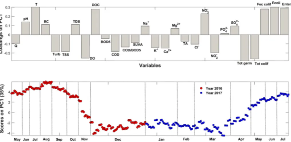
PCA revealed that the first component (PC1) explained about 35%, while the second component (PC2) accounted for 17% of the total variance. The two sub-mentioned components explained jointly about 52% of the total variance and were therefore considered significant for our study. In each PC plot, the loadings (column chart) and the scores (plot) are presented. Loadings represent the contributions of the 28 variables to the different components, while scores plot illustrates the potential temporal trends within analyzed samples (red spots for sam-ples collected in 2016 and blue spots for those collected in 2017).

Fig. 4shows the scores of the 285 analyzed samples and the load-ings referring to the 28 parameters on PC1. The anthropogenic (DOC, COD, NO3−and NO2−), physical (mainly T, DO, Turb, TSS), as well as all the bacteriological parameters, contribute basically to the con-struction of this PC. According to their locations on the scores plot, the 285 samples are mainly affected by the anthropogenic activities or not. In fact, samples collected during winter season and high overflow periods (from December 2016 to March 2017) present negative scores while samples collected during Low-Water periods (from May to No-vember of 2016 and April to July of 2017) have positive scores with some variation between year 2016 and 2017.

The physical variables essentially implicated in this discrimination on PC1 are, water temperature (T) and dissolved oxygen (DO), which are considered as key water quality indicators (Sánchez et al., 2007), as well as turbidity (Turb) and total suspended solids (TSS) measurements. Checking the scores on PC1, a classical trend can be noticed on a temporal basis according to the water temperature. This temperature profile is reasonable where an increasing trend can be seen during summer period with decreasing scores during fall and winter seasons (Alberto et al., 2001). Concerning the DO levels, high scores are oc-curring from December 2016 to March 2017, while a decreasing trend is detected during summer time. In fact, such results are expected since these two parameters are inversely correlated and oxygen solubility shows a decrease as water temperature increases (Jung et al., 2016). In fact, the dissolved oxygen concentration is greater in high-water level and overflow periods due to water turbulence event (Daou et al., 2018). In addition, lower DO levels occur throughout Low-Water period since important anthropogenic inputs and low flow levels of the river con-tribute together in inhibiting natural oxygen dissolution.

When considering the scores of the 285 water samples, the con-tribution of organic components can be noticed. TSS and turbidity are influenced by the total discharge of the river and increase during flood event when higher erosion rates are observed (El Azzi et al., 2016). However, dissolved solids are more concentrated during summer season when only groundwater is contributing to the total discharge. In fact, the dissolved elements are diluted by surface and sub-surface runoffs during rain episodes and are therefore less concentrated during the winter season (Probst, 1992). This can explain the high levels of DOC during low-water periods. In addition, in-stream DOC production is important during low flow periods. In fact, the algal activity in spring as well as the leaf litter entering the stream in autumn can be responsible for DOC maxima during low flows (Mulholland and Hill, 1997). DOC has also been proven to increase during snowmelt periods (spring and summer) when runoff is mostly done via subsurface flow which acti-vates new soil organic matter fluxes (Laudon et al., 2004).

Our results show high levels of nitrate during low-water periods. Previous studies stipulated that nitrate can enter streams through sur-face, subsurface and groundwater flow (El Azzi et al., 2016; Goolsby et al., 2000). Thus, its concentrations generally decrease in low flow, in the summer. In the Ibrahim River, an opposite pattern was observed. This can be explained by seasonal fluctuations in the number of bacteria Fig. 3. Variations of the Ibrahim River discharge during the sampling campaign

from May 2016 to July 2017. Sampling points are represented with the circles and were collected at the outlet during high flows (every two hours) and low flows (once a week).

Table 1 Tested physico-chemical and microbiological parameters with mean values and standard deviations during the study period, at high flow and at low flow. Parameter Analytical Method Mean ± Standard Deviation during the study period Mean ± Standard Deviation during High-Water period Mean ± Standard Deviation during Low-Water period pH pH Meter CyberScan pH11 part of ThermoFisherScientific Eutech NF T 90-008 8.04 ± 0.40 7.96 ± 0.43 8.20 ± 0.28 Conductivity (EC, µS/cm) Conductivity Meter CyberScan Con11 part of ThermoFisherScientific Eutech NF EN 27888 324.34 ± 72.37 308.58 ± 79.56 356.88 ± 37.92 Temperature (T, °C) Checktemp1 Pocket Thermometer Hanna 15.85 ± 4.22 13.33 ± 2.39 21.05 ± 1.58 Dissolved Oxygen (DO, mg/L) Oxygen meter Lutron DO5510 NF EN 25814 (March 1993) 7.58 ± 1.26 8.23 ± 0.88 6.24 ± 0.76 Turbidity (Turb, NTU) Turbidimeter TB1 Velp Scientifica NF EN ISO 7027 (March 2007) 31.91 ± 38.13 42.44 ± 42.39 10.19 ± 7.33 Total Dissolved Solids (TDS, mg/L) TDS meter (hold) HM digital AOAC 920.193 105.41 ± 22.86 100.39 ± 24.85 115.79 ± 13.00 Total Suspended Solids (TSS, mg/L) NF EN 872 (June 2005) 32.39 ± 41.70 43.54 ± 46.55 9.36 ± 8.54 Dissolved Organic Carbon (DOC, mg/L) TOC-L SHIMADZU ISO 8245:1999 2.06 ± 0.77 1.71 ± 0.56 2.78 ± 0.63 Biochemical Oxygen Demand (BOD5, mg/L) Lovibond OxiDirect NF EN 1899-2 (May 1998) 2.19 ± 0.57 2.28 ± 0.52 2.00 ± 0.63 Chemical Oxygen Demand (COD, mg/L) Spectrometry Helios Alpha Thermo Chemetrics Kits 19.15 ± 6.88 20.49 ± 7.32 16.39 ± 4.83 Total Alkalinity (TA, mg CaCO 3 /L) Titrimetry NF T 90-036 ISO 9963-1:1994 130.81 ± 13.10 131.87 ± 15.60 128.62 ± 4.21 Specific Ultraviolet Absorbance (SUVA, L mg −1 m −1 ) Spectrometry Helios Alpha Thermo 254 nm 1.74 ± 1.40 1.869 ± 1.18 1.50 ± 1.77 Dissolved Sodium (Na +,mg/L) Flame photometry M410 Sherwood Scientific NF T 90-019 3.88 ± 2.04 3.39 ± 2.11 4.90 ± 1.44 Dissolved Potassium (K +,mg/L) Flame photometry M410 Sherwood Scientific NF T 90-019 1.02 ± 0.75 1.18 ± 0.86 0.69 ± 0.13 Dissolved Calcium (Ca ++ ,mg/L) Titrimetry NF T 90-016 ISO 6058-1984 48.47 ± 6.92 50.65 ± 7.14 43.99 ± 3.40 Dissolved Magnesium (Mg ++ ,mg/L) Titrimetry ISO 6059-1984 8.49 ± 4.09 7.46 ± 4.16 10.62 ± 2.98 Dissolved Chloride (Cl −,mg/L) Titrimetry NF T 90-014 ISO 9297-1989 10.54 ± 3.10 11.25 ± 3.41 9.06 ± 1.47 Dissolved Nitrate (NO 3 −,mg/L) Spectrometry Helios Alpha Thermo NF T 90-045 ISO 7890-3:1988 0.82 ± 1.08 0.39 ± 0.54 1.70 ± 1.36 Dissolved Nitrite (NO 2 −,mg/L) Spectrometry Helios Alpha Thermo ISO 6777-1984 0.06 ± 0.05 0.07 ± 0.06 0.02 ± 0.02 Dissolved Phosphate (PO 4 3−,mg/L) Spectrometry Helios Alpha Thermo NF T 90-023 0.048 ± 0.05 0.03 ± 0.03 0.05 ± 0.06 Dissolved Sulfate (SO 4 2−,mg/L) Spectrometry Helios Alpha Thermo NF T 90-040 13.05 ± 6.85 11.64 ± 7.12 15.95 ± 5.19 Total Germs (CFU/100 mL) ISO 6222:1999(E) 294.70 ± 1.03 10 3 344.13 ± 0.82 10 3 192.67 ± 0.53 10 3 Total Coliforms NL ISO 9308-1:2012 and ISO 7899-2:2000(E) 2.60 ± 0.78 10 3 2.89 ± 0.75 10 3 2.00 ± 0.38 10 3 Fecal Coliforms Escherichia coli Enterococcus (CFU/100 mL) 1.31 ± 0.56 10 3 10.37 ± 11.06 9.21 ± 8.78 1.02 ± 0.34 10 3 4.20 ± 6.10 4.35 ± 4.17 1.89 ± 0.45 10 3 23.11 ± 7.53 19.25 ± 7.12

and benthic microalgae colonizing the bed sediments and influencing the oxygen and nutrient levels at the sediment-water interface (Rysgaard et al., 1995). In summer, oxygen production by these po-pulations increases the O2penetration in sediments improving the flux of inorganic nitrogen from sediments to overlying water (Rasmussen and Jørgensen, 1992; Rysgaard et al., 1995). Previous studies also proved that, during sunny days, O2 from benthic photosynthesis re-duces denitrification by more than 60% (Christensen et al., 1990). During winter season, nitrate arriving to the mainstream via surface, subsurface and groundwater flows was probably directed into the se-diment by benthic assimilation in the surface layers and denitrification in the deeper sediment layers (Rysgaard et al., 1995).

The detected high rates of nitrite may originate from anthropogenic inputs and agricultural practices. In fact, fertilizer applications are common on the Ibrahim basin agricultural fields, particularly near the river mouth, as seen in Fig. 1(Daou et al., 2016; Razmkhah et al., 2010). Nitrites present higher levels during autumn and winter seasons which confirms the important fluxes of organic material from the soil after rain events and their slow mineralization during these seasons (Heral et al., 1982).

These observations are endorsed by the bacteriological results. In fact, the low-water period is more affected by fecal contamination (the average mean values during the study period are as follow 1.31 ± 0.56 103_{CFU/100 mL for Fecal coliforms, 10.37 ± 11.06 CFU/100 mL for} Escherichia coli and 9.21 ± 8.78 CFU/100 mL for Enterococcus) due to anthropogenic inputs and/or concentration factor as mentioned above.

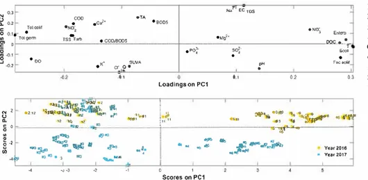
Besides, the high-water period is marked by autochthonous germs (the mean values during the study period are as follow 294.70 ± 1.03 103_{CFU/100 mL for Total germs and 2.60 ± 0.78 10}3_{CFU/100 mL for} Total coliforms) due to dilution factor and/or massive soil leaching. This bacterial profile does not only reveal the seasonal impact but also clarifies the anthropogenic evolution and consequently its effect on the water balance disturbance.Fig. 5shows the scores of the 285 analyzed samples and the loadings referring to the 28 parameters on PC2. This second component is mainly described by mineral parameters (EC, TDS, Na+_{, TA, K}+_{and Cl}−_{). Moreover, Q, pH and SUVA have also higher} loadings than other parameters.

In this component, significant annual variation is detected when comparing 2016–2017. In fact, PC2 showed decreasing scores in 2017 as compared to 2016. This decrease can be explained by the higher precipitations in 2017 as compared to 2016 which might have led to different erosion and dilution patterns. It can also be related to the Ibrahim basin’s structure consisting mainly of Jurassic and Cretaceous limestones leading to significant soil leaching during high-water sea-sons which can affect the mineral composition and pH of water, which is extremely influenced by the geological nature of the soil (Daou et al., 2013). This temporal variation is mainly perceptible in March and April 2017 when we witnessed the highest discharges (reaching 60.29 m3 s−1_{) of the study period. The Ibrahim River is polluted by mineral} discharges from industrial activities in its neighborhoods essentially marble industries, as well as by anthropogenic contaminants from surrounding areas. Moreover, the TDS measure, which refers mainly to Fig. 4. Scores of the 285 samples on the Ibrahim River outlet (red spots for samples taken in 2016 and blue spots for samples taken in 2017) and loadings of the 28 tested parameters on PC1. (For interpretation of the references to colour in this figure legend, the reader is referred to the web version of this article.)

Fig. 5. Scores of the 285 samples on the Ibrahim River outlet (red spots for samples taken in 2016 and blue spots for samples taken in 2017) and loadings of the 28 tested parameters on PC2. (For interpretation of the references to colour in this figure legend, the reader is referred to the web version of this article.)

000 OTA

.

.cJ• Toloollf _�Oi

.

-TO<gem> rss ft.rt) _{• OOOJSOOS} • 00

.

_K. SWA a-

,-

o•

.o,,

.. 2 u tl.2_12 1ilt�-1_�f�•2 ll>!i.!:L"'-.��, :,:�tQ� �

_m

_:

_:

_w

₁₁

₁

g

•

.. ..

3-2

"'

Table 2

,

,

"'

_{it;l;:R ..}

'"

_{__}

Ç

�a

-:;,,,

.

a) a:$. 3 "3

..

• 3

..

olj>Ol Jf""

--�

·

...

-

�

·2

.,

�T_• ec TOS •eoos •NOj _Enlero

.

,.

,..

.

�C.•·-;--

�

.

s&,·

.

-t'

Fe<cell o., 0.2 O.l Loadings on PC1

1

i�

\SW'O \lo tl01,:P

:

:

(

�

�

�-

..

,.,

..

!

1111 •111

..

.

.

,

_.,·-�t

�'"�--

..,

,:.-tt

-.o

.,

_'r,

_'i1.

0< M _{., ,If;}

.. ....

.

_Ycar2010 Yttir 2017 0 1 Scores on PC1

Correlation analysis between the nineteen shortlisted parameters.

Q pH T EC TDS 00 DOC 8005 SUVA No' K' TA

a

Q 1 pH 0.03 1 T -0.27 0.43 EC -0.45 -0.20 0.24 TDS -0.45 -0.20 0.24 0.99 00 0.28 -0.20 -0.83 -0.45 -0.45 1 DOC -0.36 0.48 0.82 0.32 0.32 -0.67 80D5 -0.15 -033 -0.15 0.13 0.13 -0.14 -0.07 l SWA 0.21 0.22 -0.18 -0.42 -0.43 031 -0.20 -0.31 l No' -0.48 -0.46 0.24 0.72 0.73 -0.42 0.24 0.19 -0.42 l' 0.29 -0.03 -0.43 -0.53 -0.52 0.67 -038 -0.26 0.14 -OA0 TA -0.40 -0.20 -0.32 0.48 0.49 0.21 -0.12 -0.01 -0.10 0.32 0.13

cr

0.60 0.11 -0.31 -0.39 -0.38 0.54 -0.28 -0.31 0.22 -0.44 0.46 -0.14 1 NOi -0.27 0.14 0.64 0.38 0.40 -0.73 0.58 0.09 -0.44 0.46 -0.32 -0.07 -0.43 Totprms 0.09 -0.43 -0.88 -0.12 -0.12 0.72 -0.76 0.21 0.11 -0.16 039 0.33 0.26 To1<x,II 0.12 -0.56 -0.79 -0.10 -0.11 0.61 -0.70 0.16 0.06 0.01 OAO 0.32 0.18 Foa,olf -0.U 0.57 0.88 0.10 0.10 -0.61 0.85 -0.26 -0.04 0.03 -0.23 -031 -0.07 Eco/1 -0.34 OAS 0.92 0.26 0.26 -0.74 0.85 -0.17 -0.16 0.25 -0.37 -0.19 -0.32 Enuro -0.37 0.39 0.88 0.38 0.38

.o.n

0.85 -0.09 -0.21 0.32 -0.40 -0.10 -0.33

Shaded areas only point out the parameters that showed a correlation of R > 0.7.

o.,��---�---�-----�---_.-� l)H _Fecool:f N u Q. 0.2 •o s ♦I( N03 � 01---t---� C ,; � -0.2� ..J _Toteolif -0.• -0.3 -02 -0.1

'"

800>

.

0 Loadings on PC1 0 Scores on PC1 (32%) o., 02 0,3 04

Fig. 6. Scores of the 285 samples on the Ibrahim River outlet (yellow spots for 2016 and blue spots for 2017; 1: January; 2: February; 3: March; 4: April; 5: May; 6: June; 7: July; 8: August; 9: September; 10:

October; 11: November; 12: December) and loadings of the 28 tested parameters on PCl vs PC2 plot. (For interpretation of the references to colour in this figure legend, the reader is referred to the web version of this article.)

N�• Totprms Tota,11 Foaolff Ea,/i EnlG't>

1 R 1 > 0.7 (strongly correlated) -0.58 1 -0.47 0.84 0.48 -0.82 -0.74 0.65 -0.88 -0.78 0.90 0.63 -0.79 -0.70 0.87 0.89

Fig. 7. Scores of the 285 samples on the Ibrahim River outlet (yellow spots for 2016 and blue spots for 2017; 1: January; 2: February; 3: March; 4: April; 5: May; 6: June; 7: July; 8: August; 9: September; 10:

October; 11: November; 12: December) and loadings of the 10 shortlisted parameters on PCl vs PC2 plot. (For interpretation of the references to colour in this figure legend, the reader is referred to the web version of this article.)

various rninerals, salts, metals, cations and anions present in water, besides organic substances contained in water (Weber-Scannell and

Duffy, 2007), is a major parameter implicated in this PC2.

The specific ultraviolet absorbance index SUVA which is calculated through dividing the UV absorbance value at 254 nm (m -1) by the dissolved organic carbon concentration (mg L -l ), indicates the source of organic compounds found in water (Westerhoff and Anning, 2000). Checking the scores on the PC2, lower SUVA levels are noticed during

year 2016, reaching 0.06Lmg-1 m-1 in September 2016, designating subsequently an anthropogenic hydrophilic organic matter source. On the other hand, mean values are obtained for the year 2017, fluctuating around the reference value of 4 L mg-1 m -1, which means that organic matter, during this period at the Ibrahim River outlet, originates from natural sources and is essentially composed by aromatic and hurnic substances (Hatt et al. , 2013).

River outlet station, the 285 samples were plotted according to PC1 and PC2 (Fig. 6).

This plot clearly demonstrates that the samples of the year 2016 form two well defined clusters, located in the negative quadrant of PC1 and in the positive quadrant of PC2 for the first cluster and corre-sponding to November and December 2016. While the second 2016 cluster is found in the positive quadrant of PC1 and in the positive one of PC2, referring to June, July, August, September and October 2016. However, May 2016 samples are not affected by PC2 since their scores are around 0. The discrimination between the two 2016 clusters is mainly due to bacterial indicators and organic parameters such as NO2−, NO3−and DOC. Concerning the samples of year 2017, three independent clusters are identified, classified as follow. The first cluster is situated in the negative quadrant of PC1 and in the positive quadrant of PC2, corresponding to January and February 2017. Regarding March and April 2017, scores are positioned in the negative quadrant of PC1 and PC2, essentially discriminated due to their DO, K+_{, Cl}−_{, SUVA and} Q values. Yet, the third cluster formed by samples collected on May, June and July 2017, scores are situated in the positive quadrant of PC1 and in the negative quadrant of PC2. This very-well discriminated cluster is mainly separated due to its SO42− and pH parameters. According to the variable loadings responsible for the year 2017 dis-crimination, low-water level periods and high-water level ones are classified due to differences in some mineral components’ levels, highlighting consequently a clear temporal discrimination.

3.1. Parameter selection using PCA and Pearson correlation

After performing PCA, a total of 19 parameters highly contributing to the first two principal components PC1 and PC2 were selected

(> 0.2; positively or negatively). This comprised 9 variables from PC1 (T, DO, DOC, NO3−, total germs, total coliforms, fecal coliforms, Escherichia coli and Enterococcus) and 10 variables from PC2 (Q, pH, EC, TDS, BOD5, SUVA, Na+, K+, TA and Cl−). Then, Pearson correlations were computed (Table 2) and only parameters with low correlations were considered. For highly correlated parameters, a single parameter was selected as representative of the others.

In fact, water temperature was removed since it was highly corre-lated to all bacteriological parameters. Similarly, TDS and Na+_both demonstrated high correlations with EC and were removed. On another hand, DO and DOC measures, were excluded due to their high corre-lation with the NO3−as well as with all the bacteriological parameters. Furthermore, SUVA was removed since it is a calculated parameter. Finally, the total coliforms and the fecal coliforms’ counting were se-lected among the bacteriological parameters.

This left us with 10 shortlisted variables to work with (Q, pH, EC, NO3−, total coliforms, fecal coliforms, BOD5, K+, TA and Cl−).

Additionally, a new PCA was performed on the reduced matrix and the scores of the 285 analyzed samples and the loading referring to the 10 selected parameters were then plotted according to PC1 and PC2 as shown inFig. 7(PC1 explained around 32% while the second compo-nent PC2 accounted for 26% of the total variance). This new plot leaves us with the same cluster distribution as the one previously shown in

Fig. 6, which consequently highlights the importance of the reduction of number of parameters while keeping the same classification. This will help maintain all the information and thus will allow more feasible and practicable monitoring of surface water quality (Tripathi and Kumar Singal, 2019).

9 of the parameters selected were used to apply the WQI approach for the first time on the Ibrahim River using relative weights according toTable 3. The flow parameter was disregarded since it is not con-sidered as a quality indicator.

While the average WQI is 69.037 ± 1.864 referring to a good quality range, the calculated values fluctuated between 63.125 and 73.125, as shown inFig. 8, which designates medium to good water quality (Dojlido et al., 1994; Tyagi et al., 2013). The monthly WQI average values are as follows: 69.2 ± 1.5 for May 2016, 68.8 ± 1.7 for June 2016, 68.2 ± 0.6 for July 2016, 65.3 ± 1.4 for August 2016, 67.3 ± 1.2 for September 2016, 67.8 ± 0.9 for October 2016, 70.8 ± 2.5 for November 2016, 70.6 ± 1.7 for December 2016, 69.9 ± 1.3 for January 2017, 69.1 ± 0.9 for February 2017, 68.2 ± 1.5 for March 2017, 68.7 ± 0.8 for April 2017, 68.0 ± 1.4 for May 2017, 68.9 ± 0.4 for June 2017 and 68.9 ± 0.9 for July 2017.

Comparably to the previous PCA results (Fig. 4), this trend shows a seasonal variation in the Ibrahim water quality, with a medium quality Table 3

Relative weight assigned to the 9 shortlisted para-meters used for the evaluation process.

Parameter Weight Pi pH 2 EC 3 NO3− ₁ Total coliforms 3 Fecal coliforms 3 BOD5 3 K+ ₅ TA 3 Cl− ₃

May 16 June 16 July 16 Aug 16 Sept 16 Oct 16 Nov 16 Dec 16 Jan 17 Feb 17 Mar 17 Apr 17 May 17 June 17 July 17 63 64 65 66 67 68 69 70 71 72 73 WQI (%)

4. Conclusion

The presented periodic assessment of the Ibrahim River water quality was based on a temporal measurement of various physico-chemical and bacteriological parameters. Sampling campaigns were executed on the river outlet for fifteen consecutive months, from May 2016 till July 2017. This monitoring generated complex multivariate data that needed interpretation using chemometric treatment coupled with flow dynamics and in-stream behavior knowledge. This analysis identified two principal components. The first one was characterized by organic and microbiological parameters and highlighted a temporal trend, differentiating low and high river discharges. Thus, it helped identifying the main factors responsible for the water quality variations, mainly related to anthropogenic inputs and flood events. The second component was mainly influenced by mineral variables and showed a clear annual discrimination. It is noticeable that mineral parameters implicated in this discrimination were not only due to natural events such as soil erosion and leaching but also to anthropogenic activities. To reduce the total number of parameters monitored in the future, in-fluential quality indicators were identified. More specifically, PCA and Pearson correlations efficiently rendered important data reduction as it proposed only 10 parameters (Q, pH, EC, NO3−, total coliforms, fecal coliforms, BOD5, K+_{, TA and Cl}−_{) to assess temporal variations in the} Ibrahim river water quality. These shortlisted parameters, excluding the flow Q, were then used to calculate the water quality index of the Ibrahim River outlet. With an average of 69.0 ± 1.9, the IWQI values ranged between 63.1 and 73.1 referring to medium to good water quality thus showing a temporal quality variation. This study conducted on the Ibrahim River outlet can lead to future assessments of this river. Moreover, this methodology could be extended to the monitoring of the water quality in similar rivers.

Acknowledgements

This project has been partly jointly funded with the support of the National Council for Scientific Research in Lebanon CNRS-L and the Holy Spirit University of Kaslik (USEK). We give special thanks to the Lebanese-French Environmental Observatory O-LIFE (CNRS-L, CNRS-F, Lebanese and French Universities), the National Center for Remote Sensing CNRS Mansourieh, the Litani River Authority LRA, the Lebanese Agricultural Research Institute LARI Fanar and the National Center for Marine Sciences CNRS Jounieh for their technical assistance as well as their scientific support.

Appendix A. Supplementary data

Supplementary data to this article can be found online athttps:// doi.org/10.1016/j.ecolind.2019.04.061.

References

Abboud, M., 2002. Ibrahim River: A Case Study for Investigating Vegetation Patterns and Assessing Riparian Habitats. Master of Science. Department of Plant Sciences, American University of Beirut, Riad El-Solh, Beirut, pp. 111.

Abu-Jawdeh, G., Laria, S., Bourahla, A., 2000. LIBAN: enjeux et politiques d’environne-ment et de développed’environne-ment durable. Éditions du Programme des Nations-Unies pour l’Environnement/Plan Bleu/Centre d’Activités Régionales, Beyrouth, pp. 54.

Ahoussi, K.E., Koffi, Y.B., Kouassi, A.M., Soro, G., Soro, N., Biémi, J., 2012. Caractérisation physico-chimique et bactériologique des ressources en eau des localités situées aux abords de la lagune ébrié dans la commune de marcory (district d’abidjan, côte ivoire): cas du village d’abia koumassi. Eur. J. Sci. Res. 89 (3), 359–383.

Alberto, W.D., del Pilar, D.M., Valeria, A.M., Fabiana, P.S., Cecilia, H.A., de los Ángeles, B.M., 2001. Pattern recognition techniques for the evaluation of spatial and temporal variations in water quality. A case study: Suquı́a River Basin (Córdoba–Argentina). Water Res. 35 (12), 2881–2894.

Assaf, H., Saadeh, M., 2008. Assessing water quality management options in the Upper Litani Basin, Lebanon, using an integrated GIS-based decision support system. Environ. Modell. Software 23 (10–11), 1327–1337.

Assaker, A., 2016. Hydrologie et biogéochimie du bassin versant du fleuve Ibrahim: Un observatoire du fonctionnement de la zone critique au Liban (Doctoral dissertation). Barakat, A., El Baghdadi, M., Rais, J., Aghezzaf, B., Slassi, M., 2016. Assessment of spatial and seasonal water quality variation of Oum Er Rbia River (Morocco) using multi-variate statistical techniques. Int. Soil Water Conserv. Res. 4 (4), 284–292.https:// doi.org/10.1016/j.iswcr.2016.11.002.

Bou Saab, H., Nassif, N., El Samrani, A.G., Daoud, R., Medawar, S., Ouaïni, N., 2007. Survey of bacteriological surface water quality (Nahr Ibrahim river, Lebanon). Rev. Sci. Eau. 20 (2), 341–352.

Chamas, L., Akl, G., Hamdan, O., Kaskas, A., Abu Salman, R., Nasr, W., Mina, G., Kallas, L., El-Fadel, M., Huybrechts, E., Alayan, N., Karam, J., 2001. State of the Environment Report. Ministry of Environnement, Beirut, pp. 283.

Christensen, P.B., Nielsen, L.P., Sørensen, J., Revsbech, N.P., 1990. Denitrification in nitrate-rich streams: diurnal and seasonal variation related to benthic oxygen meta-bolism. Limnol. Oceanogr. 35 (3), 640–651.https://doi.org/10.4319/lo.1990.35.3. 0640.

Daou, C., Nabbout, R., Kassouf, A., 2016. Spatial and temporal assessment of surface water quality in the Arka River, Akkar, Lebanon. Environ. Monit. Assessm. 188 (12), 684.

Daou, C., Salloum, M., Legube, B., Kassouf, A., Ouaini, N., 2018. Characterization of spatial and temporal patterns in surface water quality: a case study of four major Lebanese rivers. Environ. Monit. Assess. 190 (8), 485.

Daou, C., Salloum, M., Mouneimne, A.H., Legube, B., Ouaini, N., 2013.

Multidimensionnal analysis of two Lebanese surface water quality: Ibrahim and el-Kalb rivers. J. Appl. Sci. Res. 9 (4), 2777–2787.

De La Mora-Orozco, C., Flores-Lopez, H., Rubio-Arias, H., Chavez-Duran, A., Ochoa-Rivero, J., 2017. Developing a water quality index (WQI) for an irrigation dam. Int. J. Environ. Res. Public Health 14 (5), 439.

Demirak, A., Yilmaz, F., Tuna, A.L., Ozdemir, N., 2006. Heavy metals in water, sediment and tissues of Leuciscus cephalus from a stream in southwestern Turkey. Chemosphere 63 (9), 1451–1458.

Dojlido, J., Raniszewski, J., Woyciechowska, J., 1994. Water quality index applied to rivers in the Vistula river basin in Poland. Environ. Monit. Assess. 33 (1), 33–42.

El Amil, R., Oudwane, J., 2000. Les ressources en eau et en matières minérales du bassin versant du Nahr Ibrahim. Mémoire de fin d’études en maîtrise de biologie, Faculté des Sciences II, Université Libanaise, Fanar, Liban, pp. 42.

El Azzi, D., Probst, J.L., Teisserenc, R., Merlina, G., Baqué, D., Julien, F., Guiresse, M., 2016. Trace element and pesticide dynamics during a flood event in the Save agri-cultural watershed: Soil-river transfer pathways and controlling factors. Water Air Soil Pollut. 227 (12), 442.

El Azzi, D., Viers, J., Guiresse, M., Probst, A., Aubert, D., Caparros, J., Probst, J.L., 2013. Origin and fate of copper in a small Mediterranean vineyard catchment: New insights from combined chemical extraction and δ65Cu isotopic composition. Sci. Total Environ. 463, 91–101.

El-Fadel, M., Zeinati, M., Jamali, D., 2000. Water resources in Lebanon: characterization, water balance and constraints. Int. J. Water Resour. Dev. 16 (4), 615–638.

Fan, X., Cui, B., Zhao, H., Zhang, Z., Zhang, H., 2010. Assessment of river water quality in Pearl River Delta using multivariate statistical techniques. Procedia Environ. Sci. 2, 1220–1234.

Fitzpatrick, A., Fox, J., Leung, K., 2001. Environmental Baseline Survey of the Nahr Ibrahim, Lebanon. Masters of Engineering. Department of Civil and Environmental Engineering, Massachusetts Institute of Technology, Cambridge, MA, États-Unis, pp. 114.

Giannakopoulos, C., Le Sager, P., Bindi, M., Moriondo, M., Kostopoulou, E., Goodess, C.M., 2009. Climatic changes and associated impacts in the Mediterranean resulting from a 2 C global warming. Global Planet. Change 68 (3), 209–224.

Goolsby, D.A., Battaglin, W.A., Aulenbach, B.T., Hooper, R.P., 2000. Nitrogen flux and sources in the Mississippi River Basin. Sci. Total Environ. 248 (2), 75–86.

Hatt, J.W., Germain, E., Judd, S.J., 2013. Powdered activated carbon-microfiltration for waste-water reuse. Sep. Sci. Technol. 48 (5), 690–698.

Hébert, S., Légaré, S., 2000. Suivi de la qualité des rivières et petits cours d’eau. Québec, Direction du suivi de l’état de l’environnement, ministère de l’Environnement, en-virodoq no ENV-2001-0141, rapport no QE-123, 24p. et, 3.

Heral, M., Razet, D., Deslous-Paoli, J.-M., Berthome, J.-P., Garnier, J., 1982. Caracteristiques saisonnieres de l hydrobiologie du complexe estuariende Marennes-Oleron (France). Revue des Travaux de l’Institut des Pêches Maritimes 46 (2), 97–119.

Houri, A., El Jeblawi, S.W., 2007. Water quality assessment of Lebanese coastal rivers during dry season and pollution load into the Mediterranean Sea. J. Water Health 5 (4), 615–623.

Jung, K.Y., Lee, K.-L., Im, T.H., Lee, I.J., Kim, S., Han, K.-Y., Ahn, J.M., 2016. Evaluation of water quality for the Nakdong River watershed using multivariate analysis. Environ. Technol. Innovation 5, 67–82.

Kabbara, N., Benkhelil, J., Awad, M., Barale, V., 2008. Monitoring water quality in the

during low-water periods and a good one in high-water periods. The IWQI should be further tested on the Ibrahim watershed. This technique can be extrapolated to other river basins, characterizing spatial and/or temporal variability. Such studies, reflecting t he ag-gregate influence o f m ultiple p hysico-chemical a s w ell a s micro-biological parameters, integrating therefore several variables in a spe-cific value, can be accomplished in forthcoming assessments to support the evaluation of various management strategies and monitoring deci-sions (Massoud, 2012).

coastal area of Tripoli (Lebanon) using high-resolution satellite data. ISPRS J. Photogramm. Remote Sens. 63 (5), 488–495.

Kannel, P.R., Lee, S., Lee, Y.S., Kanel, S.R., Khan, S.P., 2007. Application of water quality indices and dissolved oxygen as indicators for river water classification and urban impact assessment. Environ. Monit. Assess. 132 (1–3), 93–110.

Koçer, M.A.T., Sevgili, H., 2014. Parameters selection for water quality index in the as-sessment of the environmental impacts of land-based trout farms. Ecol. Ind. 36, 672–681.

Lamizana-Diallo, M. B. (2008). Évaluation de la qualité physico-chimique de l’eau d’un cours d’eau temporaire du Burkina Faso-Le cas de Massili dans le Kadiogo. Laudon, H., Köhler, S., Buffam, I., 2004. Seasonal TOC export from seven boreal

catch-ments in northern Sweden. Aquat. Sci. 66 (2), 223–230.https://doi.org/10.1007/ s00027-004-0700-2.

Lumb, A., Sharma, T.C., Bibeault, J.F., 2011. A review of genesis and evolution of water quality index (WQI) and some future directions. Water Qual. Exposure Health 3 (1), 11–24.

Massoud, M.A., 2012. Assessment of water quality along a recreational section of the Damour River in Lebanon using the water quality index. Environ. Monit. Assess. 184 (7), 4151–4160.

Mulholland, P.J., Hill, W.R., 1997. Seasonal patterns in streamwater nutrient and dis-solved organic carbon concentrations: separating catchment flow path and in-stream effects. Water Resour. Res. 33 (6), 1297–1306.

Ouhmidou, M., Chahlaoui, A., 2015. Caractérisation bactériologique des eaux du barrage Hassan Addakhil (ERRACHIDIA-MAROC). LARHYSS J. (22), 183–196 ISSN 1112-3680.

Papazian, H.S., 1981. A Hydrogeological Study of the Nahr Ibrahim Basin in the Vicinity of the Paper Mill Project of Indevco in Lebanon.

Pesce, S.F., Wunderlin, D.A., 2000. Use of water quality indices to verify the impact of Córdoba City (Argentina) on Suquı́a River. Water Res. 34 (11), 2915–2926. Probst, J.-L. (1992). Géochimie et hydrologie de l’érosion continentale. Mécanismes, bilan

global actuel et fluctuations au cours des 500 derniers millions d’années. (Vol. 94). Persée-Portail des revues scientifiques en SHS.

Ramakrishnaiah, C.R., Sadashivaiah, C., Ranganna, G., 2009. Assessment of Water Quality Index for the Groundwater in Tumkur Taluk, Karnataka State, India [Research article]. Eur.-J. Chem. 6 (2), 523–530.https://doi.org/10.1155/2009/ 757424.

Rasmussen, H., Jørgensen, B.B., 1992. Microelectrode studies of seasonal oxygen uptake in a coastal sediment: role of molecular diffusion. Marine Ecol. Progr. Series. Oldendorf 81 (3), 289–303.

Razmkhah, H., Abrishamchi, A., Torkian, A., 2010. Evaluation of spatial and temporal variation in water quality by pattern recognition techniques: a case study on Jajrood River (Tehran, Iran). J. Environ. Manage. 91 (4), 852–860.

Reza, R., Singh, G., 2010. Assessment of ground water quality status by using water quality index method in Orissa, India. World Appl. Sci. J. 9 (12), 1392–1397.

Ringnér, M., 2008. What is principal component analysis? Nat. Biotechnol. 26 (3), 303.

R., 2007. Use of the water quality index and dissolved oxygen deficit as simple in-dicators of watersheds pollution. Ecol. Ind. 7 (2), 315–328.

Srebotnjak, T., Carr, G., de Sherbinin, A., Rickwood, C., 2012. A global Water Quality Index and hot-deck imputation of missing data. Ecol. Ind. 17, 108–119.

Sharma, M., Kansal, A., Jain, S., Sharma, P., 2015. Application of multivariate statistical techniques in determining the spatial temporal water quality variation of ganga and yamuna rivers present in Uttarakhand State, India. Water Qual. Exposure Health 7 (4), 567–581.

Shrestha, S., Kazama, F., 2007. Assessment of surface water quality using multivariate statistical techniques: a case study of the Fuji river basin, Japan. Environ. Modell. Software 22 (4), 464–475.

Simeonov, V., Stratis, J.A., Samara, C., Zachariadis, G., Voutsa, D., Anthemidis, A., Kouimtzis, T., 2003. Assessment of the surface water quality in Northern Greece. Water Res. 37 (17), 4119–4124.

Singh, K.P., Malik, A., Mohan, D., Sinha, S., 2004. Multivariate statistical techniques for the evaluation of spatial and temporal variations in water quality of Gomti River (India)-a case study. Water Res. 38 (18), 3980–3992.

SOER (State Of Environment Report), 2001. Ministry of Environment and the Lebanese Environment and Development Observatory. ECODIT.

Sutadian, A.D., Muttil, N., Yilmaz, A.G., Perera, B.J.C., 2018. Development of a water quality index for rivers in West Java Province, Indonesia. Ecol. Indic. 85, 966–982.

https://doi.org/10.1016/j.ecolind.2017.11.049.

Taghavi, L., Merlina, G., Probst, J.L., 2011. The role of storm flows in concentration of pesticides associated with particulate and dissolved fractions as a threat to aquatic ecosystems-case study: the agricultural watershed of Save river (Southwest of France). Knowledge Manage. Aquatic Ecosyst. 400, 06.

Tripathi, M., Kumar Singal, S., 2019. Use of principal component analysis for parameter selection for development of a novel water quality index: a case study of river Ganga India. Ecol. Indic. 96 (1), 430–436.

Tyagi, S., Sharma, B., Singh, P., Dobhal, R., 2013. Water quality assessment in terms of water quality index. Am. J. Water Resour. 1 (3), 34–38.

Weber-Scannell, P.K., Duffy, L.K., 2007. Effects of total dissolved solids on aquatic or-ganism: a review of literature and recommendation for salmonid species. Am. J. Environ. Sci.

Westerhoff, P., Anning, D., 2000. Concentrations and characteristics of organic carbon in surface water in Arizona: influence of urbanization. J. Hydrol. 236 (3–4), 202–222.

Wold, S., Esbensen, K., Geladi, P., 1987. Principal component analysis. Chemometr. Intell. Lab. Syst. 2 (1–3), 37–52.

Rodier, J., Legube, B., Merlet, N., & Brunet, R. (2009). L'analyse de l'eau-9e éd.: Eaux naturelles, eaux résiduaires, eau de mer. Dunod.

Rysgaard, S., Christensen, P., Nielsen, L., 1995. Seasonal variation in nitrification and denitrification in estuarine sediment colonized by benthic microalgae and bio-turbating infauna. Mar. Ecol. Prog. Ser. 126, 111–121.