Quantifying nitrogen losses in oil palm plantations: models and challenges
Texte intégral
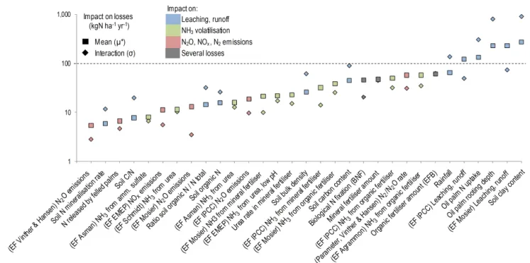
Figure

Documents relatifs
Examples are nutrient management, water level management on peat soils, pest control, residue treatment (EFB, POME and nutshells), energy efficiency in oil mills
Rules are applied on annual values, such as annual scores of losses, fraction of soil covered, annual fertiliser application rate, N lack or excess at least over one
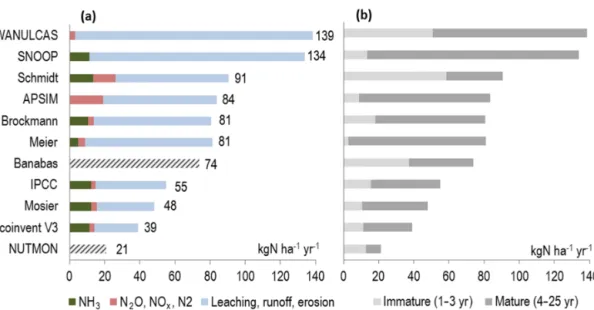
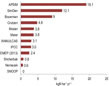
The results represented mostly losses through leaching due to low values for runoff losses (< 0.06 kg N ha −1 yr −1 ). The hatched bars represent calculations which include
We designed it to be easily implementable with available data on climate and soil conditions, and sensitive to practices such as fertiliser application (type, rate and timing),
Smallholders including family farms Africa « Palm grove » Oil palm smallholdings Africa Family farms Africa Traditional extraction by treading with water. Africa
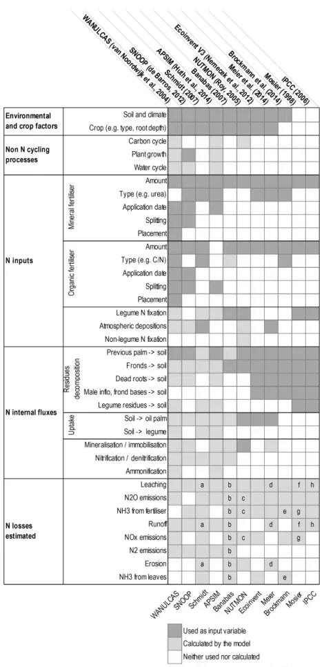
While a number of models exist to estimate nitrogen (N) losses from agricultural fields, they mostly pertain to temperate climate conditions and annual crops.. The lack of
To quantify the effects of rainforest to oil palm conversion on carbon, water and energy fluxes, a new plant functional type (PFT) and special multilayer structure are
We calculated a simplified annual gross margin of mature plantation, considering the main cost and benefits of the 3 oil palm cropping systems and the 2 rubber cropping
