O
pen
A
rchive
T
OULOUSE
A
rchive
O
uverte (
OATAO
)
OATAO is an open access repository that collects the work of Toulouse researchers and
makes it freely available over the web where possible.
This is an author-deposited version published in:
http://oatao.univ-toulouse.fr/
Eprints ID : 16005
To link to this article :
DOI:10.1016/j.jcp.2016.06.013
URL :
http://dx.doi.org/10.1016/j.jcp.2016.06.013
To cite this version :
Lepilliez, Mathieu and Popescu, Elena Roxana and Gibou, Frédéric
and Tanguy, Sébastien On two-phase flow solvers in irregular
domains with contact line. (2016) Journal of Computational Physics,
vol. 321. pp. 1217-1251. ISSN 0021-9991
Any correspondence concerning this service should be sent to the repository
administrator:
[email protected]
On
two-phase
flow
solvers
in
irregular
domains
with
contact
line
Mathieu Lepilliez
a,b,c,
Elena
Roxana Popescu
a,
Frederic Gibou
d,e,
Sébastien Tanguy
a,∗aInstitutdeMécaniquedesFluidesdeToulouse,2bisalléeduProfesseurCamilleSoula,31400Toulouse,France bCentreNationald’EtudesSpatiales,18AvenueEdouardBelin,31401ToulouseCedex9,France
cAirbusDéfence& Space,31AvenuedesCosmonautes,31402ToulouseCedex4,France
dDepartmentofMechanicalEngineering,UniversityofCalifornia,SantaBarbara,CA93106-5070,UnitedStates eDepartmentofComputerScience,UniversityofCalifornia,SantaBarbara,CA93106-5110,UnitedStates
Keywords:
Sharpinterfacemethods Irregulardomains Implicitviscosity Contactlines Levelsetmethod Ghost-FluidMethod
Wepresentnumericalmethods thatenablethedirect numericalsimulationoftwo-phase flowsinirregulardomains.Amethodispresentedtoaccountforsurfacetensioneffectsin ameshcellcontainingatriplelinebetweentheliquid,gasandsolidphases.Ournumerical methodis based onthelevel-set method tocapture theliquid–gasinterfaceand onthe single-phaseNavier–Stokessolverinirregulardomainproposedin[35]toimposethesolid boundaryinanEulerianframework.Wealsopresentastrategyfortheimplicittreatment oftheviscoustermandhowtoimposebothaNeumannboundaryconditionandajump conditionwhensolving for thepressure field. Special careisgiven on howto takeinto accountthe contactangle, the no-slipboundary condition for thevelocity fieldand the volumeforces.Finally,we presentnumericalresults intwoandthreespatialdimensions evaluatingoursimulationswithseveralbenchmarks.
1. Introduction
Multiphaseflows areubiquitous inmostmodern processing technologyand arecritical to theunderstandingofawide
range of physical and biological phenomena. Consequently, the design of numerical methods enabling the simulation of
multiphaseflowsisthesubjectofintenseresearch.Whenconsideringsolidboundaries,explicitdescriptionsofthegeometry
have demonstratedresults ofsuperior accuracy inthecaseofone-phaseflows,whencompared toimplicitrepresentations
ofthegeometry.Indeed, body-fittedgridscanbeconstructedtoenabletheaccuratetreatmentofboundaryconditionsand
to capture the rapid variations of the solution near walls, e.g. the turbulent boundary layer in high speed flows. In the
caseofmultiphaseflows, however, body-fittedapproachesareless practicalsinceconformingmeshmustbereconstructed
several time duringthe courseofa simulation.This is,for example, thecase ofthe simulationofbubbly flows or sprays,
where the fluid interface can be strongly deformed and stretched. The automatic meshing necessary in such cases is a
difficulttaskandinturn,theresulting meshcouldlackthequalityneeded toguaranteeaccuratenumericalresults.
Since the pioneer work of Peskin [38], introducing the immersed boundary method, an important research effort has
been devotedtothedevelopment ofEulerianfluidsolversinirregulardomains.Thesemethodshavetheadvantagethatno
remeshingisnecessaryduringthecourseofasimulationinthecaseofuniformgrids.Ifadaptive gridsareemployed,then
the remeshingisstraightforward sincethe free boundaryis embeddedinthe grid. Twoclasses ofmethodshave emerged
in the Eulerian framework: ‘delta’ formulations, where the Dirac distribution representing surface forces is approximated
by a regularized function [54] (and the references therein) and ‘sharp’ approaches, where jump conditions at the free
boundaryareenforcedatthediscretelevel [15,19,22,32,40,43,52,53,64,66](andthereferencestherein).Formulationsbased
onregularizedDiracdistributionsprovideapathwaytoeasilyextendsingle-phasetomultiphasesolvers[8,49].Ontheother
hand, these methods sufferfromdrawbacks that limittheir useinsome applications due totheinherent smearingofthe
solution near interfaces. Althoughefficient adaptive meshrefinement techniques [2,20] can help reduce the extent ofthe
smearingbyimposingincreasedresolutionwhereneeded, ‘sharp’numericalmethodsarestilldesired insome applications.
Thesemethods,however,aredifficulttodesign duetothedifficultyofimposingboundaryconditionsimplicitly.
While several works have been presented in thelast decade on immersed boundarymethods for incompressible
one-phase flows [4,25,31,33–35,56,57,59,63,65], only afew [29,36,58] have been dedicatedto incompressible two-phase flows,
especially inthecase whereacontact lineoftheliquid–gasinterface isformedon theembedded solidboundary. Insuch
a situation, two different interfaces must bemanaged in a computational cell, and the numerical solver for the pressure
mustimpose botha jumpconditionbetween theliquidandthegasto accountfor surfacetensioneffects and aNeumann
boundarycondition betweenthefluidand thesolidphasetoimposetheno-slip boundarycondition.
An attractive immersed boundary method for one-phase flows, based on a finite volume discretization of the Laplace
operator, has been proposed in [35]. Itenables to impose solid boundary conditions on the pressure and on thevelocity
with a second-order spatial accuracy and to maintain the symmetric definite positiveness of the resulting linear system.
Consequently, standardmethodssuch asthepreconditionedconjugategradient can beused toinvertefficiently thelinear
system.
Inthispaper,we proposeto extendtheworkof[35]to themorecomplex situation oftwo-phaseflows.Indeed, toour
knowledge, only a few methods are dedicated to thenumerical simulation of multiphase flows in irregular domains. As
two-phase flows are involved, surface tension has to be accounted for, even in the case where solid, liquid and gas are
present in thesame computationalcell. To that extent, we have developed a newnumerical scheme to account for both
a pressure jumpcondition due tothesurface tensionand aNeumanncondition on thesoliddomain inthesamecells,as
described in section 3.2. This spatialdiscretization enables thetreatment of volume forces inside themesh cells that are
crossedbythecontactline.Insection3.3,specificdetailsaregivenonhowtoperformanimplicittemporaldiscretizationof
theviscoustermswithacoupledlinearsysteminvolvingallthevelocitycomponents,whileimposingthejumpconditionon
viscosity.Insection3.4,wedescribehowtoenforcetheDirichletboundaryconditiononthevelocityfieldincomputational
cells crossed by the solid boundary, in order to ensure the no-slip boundary condition. To our knowledge, solving such
a coupled system with an immersed boundary condition has never been addressed in the existing literature. Finally, we
discuss insection 3.5howtoimposetheappropriatecontactanglebyextrapolatingtheliquid–gaslevel-setfunctioninside
thesoliddomainwithaniterativePDE.
Severalbenchmarksareproposedinsection4.Inthefirstpartofsection4,one-phaseflow simulationsarepresentedin
order to compare twopossible approachesto compute theviscous terms intwo and threespatial dimensions.Next,
test-cases involvingtwo-phaseflows in acomplex geometry(dropletdeposited on aslanted wall, half-filled rotatingspherical
tank) are presented and compared to theoretical solutions in order to highlight the behavior of the proposed numerical
methods for thecomputation of the surface tensionand the volume forcesin the grid cellsthat areboth crossed bythe
liquid–gas interface and the solid boundary. Orders of accuracy are difficult to determine for such simulations, however
grid sensitivitystudiesarepresentedforallthebenchmarksinordertoascertainthatallthecomputationsconvergetothe
correct solution.
2. Equationsandstandardprojectionmethods
The Navier–Stokes equations describe the motion of fluids at the continuum level. However, their formulations and
approximations depend on how surface forcesare represented. Nevertheless, standard state-of-the-art numerical
approxi-mationsarebasedontheprojectionmethodforsingle-phaseflows,introducedbyChorin[11].
2.1. Single-phaseflows
Consider a domain Ä= Äl∪ Äs with boundary ∂Ä. The regions Äl and Äs represent the fluidand solid regions,
re-spectively. Theboundarybetweenthefluidand thesolidisdenotedbyŴs.Theincompressible Navier–Stokesequationsfor
one-phaseNewtonianflowsarewrittenas:
∇ ·
u=
0 inÄ
l,
ρ
µ ∂
u∂
t+ (
u· ∇)
u
= −∇
p+
µ
1
u+
ρ
g inÄ
l,
where t theistime,
ρ
thefluiddensity,u= (u,v,w) thevelocity field,µ
theviscosity assumed constant, p the pressure and g theaccelerationduetogravity.Fig. 1. The computational domain in the case of two-phase flows in irregular domains.
Inthecaseofsingle-phaseflows,ChorinusedtheHodgedecompositionofvectorfields,todesignathree-stageprojection method to solvetheNavier–Stokes equations[11]:first, given a velocity un at timetn=n1t,anintermediate velocity u∗
canbecomputedforatimestep1t withoutconsideringthepressurecomponent:
u∗
=
un− 1
tµ
¡
un· ∇
¢
un−
µ
1
u nρ
−
g
.
Second,thepressurefield pn+1 servesasthescalarfunctionoftheHodgedecomposition, satisfying:
∇ ·
µ ∇
p n+1ρ
=
∇ ·
u ∗1
t,
(1)withhomogeneousNeumannboundaryconditionson ∂Äandnon-homogeneousNeumannboundaryconditionon Ŵs:
ns
·
∇
pρ
¯
¯
¯
¯
Ŵ s=
ns·
¡
u∗−
us¢¯
¯
Ŵs,
where us is thespecifiedvelocity fieldon thesolid’sboundary. Finally, thefluidvelocity un+1 isdefined at thenewtime
steptn+1 astheprojectionofu∗ ontothedivergence-freespace: un+1
=
u∗− 1
t∇
pn+1
ρ
.
2.2. Two-phaseflows
Consideracomputationaldomain,Ä,thatcontainssolid,liquidandgasregionsdenotedbyÄs,Äl andÄg,respectively1
(see Fig. 1).We call Ŵ theliquid’s boundary and n its outwardnormal. Likewise, we callŴs thesolid’s boundary and ns
its outward normal. Finally, ∂Ä denotes the boundary of Ä. The incompressible Navier–Stokes equations for Newtonian
two-phase flowscanbedescribed differently, whetherthejump conditionsareconsidered asfunctionsin theentire
com-putational domain,orassharpjumpconditionslocallyappliedtothedensity,viscosityand pressurefield.Inwhatfollows,
we brieflypresentthemainformulationsthat areused, keepinginmindthatanimplicitformulationoftheviscous terms
must be favored to perform computations on irregular domains because an immersed Dirichlet boundary condition has
to beimposed on thevelocity field. Indeed, asasubcell resolution isused to compute thisboundary condition, temporal
stabilityofthecomputationcannotbeachievedbyusinganexplicittemporaldiscretization,see[18]formoredetails.
2.2.1. The“delta”formulation
The“delta”formulation[44,49]writestheNavier–Stokesequationsfortwo-phaseflowsas:
∇ ·
u=
0,
ρ
µ ∂
u∂
t+ (
u· ∇)
u
= −∇
p+
ρ
g+ ∇ ·
³
2µ
D´
+
σ κ
nδ
Ŵ,
where
σ
isthesurface tension,κ
is theinterfacelocalmeancurvature, δŴ amultidimensionalDirac distributionlocalizedattheinterface,and D therate-of-deformationtensordefinedas:
D
=
∇
u+ ∇
uT
2
.
Thedensityand theviscosityarepiecewiseconstantandonlyvaryacross theinterface.Theycanthenbedefinedas:
ρ
=
ρ
l+
HŴ(
ρ
g−
ρ
l),
µ
=
µ
l+
HŴ(
µ
g−
µ
l),
with HŴ denotingtheHeaviside distribution,equalto 1in theliquidand 0inthegasphase, withthefollowingdefinition
fordensity andviscosityjumpconditions:
[
ρ
] =
ρ
l−
ρ
g,
[
µ
] =
µ
l−
µ
g.
When applying a projection method to the “delta” formulation, one obtains thefollowing explicit discretization: first,
solveforanintermediatevelocity fieldu∗1 with
u∗1
=
un− 1
t
¡
un· ∇
¢
un−
∇ ·
³
2µ
n+1Dn´
ρ
n+1−
σ κ
n+1ρ
n+1 nδ
Ŵ−
g
.
In therestof thepaper,we omitthe subscriptson
κ
andµ
, whichare alwaysestimatedattn+1.Second, solveaPoissonequationtodetermine theHodgefield:
∇ ·
µ ∇
p n+1ρ
n+1
=
∇ ·
u ∗ 11
t.
And finallyproject u∗
1 ontothedivergence-freevelocityfield:
un+1
=
u∗1− 1
t∇
p n+1ρ
n+1.
ThisnumericalschemeisusuallyusedintheframeworkoftheContinuumSurfaceForce(CSF)model,whichrequiresthe
definitionofsmoothedfunctionsδǫ and Hǫ toapproximate theDirac andHeavisidedistributions.Theease of
implementa-tionofthismethodcomes withdrawbackofartificiallythickeningtheinterface.UnliketheCSFmodel,the“sharp”interface
approach[24,39,50]buildsasharpdiscretizationofsingularsourceterms,avoidingtheintroductionofafictitiousinterface
thickness.Some detailsonthetheoreticalequivalencebetween thejumpcondition formulationand the“delta”formulation
isdetailedin[26,27].
2.2.2. TheGhost-FluidPrimitiveviscousMethod
Asplittingontheviscous-stresstensorcanbeapplied:
∇ ·
³
2µ
D´
=
2µ
∇ ·
³
D´
+
2[
µ
]
∂
un∂
nδ
Ŵn=
µ
1
u+
2[
µ
]
³
nT· ∇
u·
n´
δ
Ŵn.
(2)
Thisleadstoanewpossibledescriptionoftheintermediatevelocity,whereajumpcondition intheviscoustermhastobe
imposed.Thereadermayfindadetaileddemonstrationofequation(2)inAppendix A.
In[24],theauthorsproposedasharpinterfacemethodforincompressibletwo-phaseflowsbasedontheprinciplesofthe
Ghost-FluidMethod[15,28].Thisapproachiswidelyused intheliterature,eventhoughitisfirst-orderaccurateforsolving
the Poisson equation withjump conditions. In [21], asecond-order approachhas been developed, but notyet applied to
Navier–Stokes equations.TheGhost-FluidMethodintroducedin[24]canbedescribedbrieflyasproposedin[26]:first,the
intermediatevelocity u∗ 2 isupdatedwith u∗2
=
un− 1
tµ
¡
un· ∇
¢
un−
µ
1
u ∗ρ
n+1−
g
.
Next, thePoissonequationforthepressureissolvedwiththeappropriatejumpcondition:
∇ ·
µ ∇
p n+1ρ
n+1
=
∇ ·
u ∗ 21
t+ ∇ ·
Ã
σ κ
+
2[
µ
]
¡
nT· ∇
u·
n¢
nρ
n+1δ
Ŵn!
.
un+1
=
u∗2−
1
tρ
n+1Ã
∇
pn+1−
µ
σ κ
+
2[
µ
]
³
nT· ∇
u·
n´
n
nδ
Ŵ!
.
Thismethodhas beendubbedtheGhost-FluidPrimitiveviscous Method(GFPM)in[26].In thisframework,the
compu-tation oftheviscousterms requiresto determineexplicitly thejump conditionon theprojected viscousstresses. As these
jumpconditionsdependonthenumericalsolution,achievingafullyimplicittemporaldiscretizationoftheviscoustermsis
notastraightforwardtaskinthecaseoftheGFPM.Dependingon whethertheCSFformulationortheGFPM formulationis
used, theintermediatevelocity inthepredictionstepisdifferent.Even thoughthesetwo methodsareformallyequivalent,
theyleadtodifferentdefinitionsofthepredictedvelocityfieldintheprojectionstep.
2.2.3. TheGhost-FluidConservativeviscousMethod
In[50],Sussmanetal.introducedanotherformulationfor theintermediatevelocityfield,which refersto asthe Ghost-FluidConservativeviscousMethod(GFCM)in[26].Inthiscase,theintermediatevelocity u∗
3 isobtainedas: u∗3
=
un− 1
tµ
¡
un· ∇
¢
un−
1ρ
n+1∇ ·
³
2µ
Dn´
−
g
.
Next, thePoissonequationissolvedtodeterminethepressure field:
∇ ·
µ ∇
p n+1ρ
n+1
=
∇ ·
u ∗ 31
t+ ∇ ·
µ
σ κ
nδ
Ŵρ
n+1
.
Finallyinthecorrectionstep,thephysicalvelocity fieldcanbedeterminedwiththepressurefieldpreviouslycomputed:
un+1
=
u∗3−
1
tρ
n+1(
∇
pn+1
−
σ κ
nδ
Ŵ).
In order to remove the O¡1x2¢
time step restriction incurred by the viscosity term, the following implicit temporal
discretization isused, referred toin thispaperasthe Ghost-FluidConservativeMethod withan Implicitscheme(GFCMI):
theintermediatevelocityu∗
4isupdatedas:
ρ
n+1u∗4− 1
t∇ ·
³
2µ
D∗´
=
ρ
n+1¡
un
− 1
t¡¡
un
· ∇
¢
un
−
g¢¢ ,
(3)which leadstoalargelinearsystemwherethethreevelocitycomponentsarecoupled.Thesubsequentstepsaresimilarto
theoneusedinGFCM,withthecomputationofthepressurefield:
∇ ·
µ ∇
p n+1ρ
n+1
=
∇ ·
u ∗ 41
t+ ∇ ·
µ
σ κ
nδ
Ŵρ
n+1
,
followed bythecorrectionstep:
un+1
=
u∗4−
1
tρ
n+1(
∇
pn+1
−
σ κ
nδ
Ŵ).
2.2.4. TheGhost-FluidSemi-ConservativeMethodFinallyin[26]theauthorsproposedasemi-conservativeformulationfordiscretizingtheviscousterm,referredtointhis
paperastheGhost-FluidSemi-Conservative MethodwithanImplicitscheme(GFSCMI).Startingwiththesplitting:
∇ · (
2µ
D)
= ∇ · (
µ
∇
u+
µ
∇
Tu)
=∇ · (
µ
∇
u)
+ ∇ · (
µ
∇
Tu)
=∇ · (
µ
∇
u)
+ ∇
Tu· ∇
µ
+
µ
∇ · (∇
Tu)
=∇ · (
µ
∇
u)
+ [
µ
]∇
Tu·
nδ
Ŵ,
where ∇ · (
µ
∇u) isaformalequivalentoftheone-phaseflow formulationofviscouseffects. Thereforeeachcomponent issolved independently fromthe others,asthe cross-termsofthe viscousterm in [
µ
]∇Tu·nδŴ are enforcedexplicitly asa
jumpcondition.Thepredictionstepis:
ρ
n+1u∗5− 1
t∇ ·
³
µ
∇
u∗5´
=
ρ
n+1Ã
un− 1
tµ
¡
un· ∇
¢
un−
g
!
.
∇ ·
µ ∇
p n+1ρ
n+1
=
∇ ·
u ∗ 51
t+ ∇ ·
à ¡
σ κ
+ [
µ
]
¡
nT· ∇
u·
n¢
n¢
ρ
n+1 nδ
Ŵ!
.
(4)Finally, thecorrectionsteptocomputethedivergencefree velocityis:
un+1
=
u∗5−
1
tρ
n+1Ã
∇
pn+1−
µ
σ κ
+ [
µ
]
¡
nT· ∇
u·
n¢
n
nδ
Ŵ!
.
(5)Remark.Theimplementationofanimplicittemporaldiscretizationoftheviscoustermsiseasierwiththismethod(GFSCMI)
than GFCMI.Indeed if GFSCMIisused,eachvelocity componentcan becomputedbysolvingasimple linearsystem
(sym-metricdefinitepositive)thatdoesnottreatcross-derivativesimplicitly.However,eventhoughGFCMItreatscross-derivatives
implicitly, afew iterations ofGauss–Seidel suffice forconvergence and theresults are superior toGFSCMI. Thesemethods
are compared in section 3.4 to offer some insight on how velocity boundary conditions should be enforced on irregular
domains.
2.2.5. Anoteonthetimestepconstraint
Letusremarkthat,unlikeGFCMI,GFSCMIdoesnotfullyremovethestabilityconstraintonthetimestepduetoviscosity,
sinceanexplicitpartdependingontheviscosityjumpconditionremainsinequation(5).Therefore,asithasbeendiscussed
in[26],astabilityconstraintdependingontheviscosityjumpconditionmustbeimposedtoensurestabilityofthemethod.
Specifically,thefollowingstandardtimestepconstraintsfortheconvectionandthesurfacetensioneffects,mustbeimposed
toensurethetemporalstabilityofthecomputation:
1
tconv=
1
x max|
u|
,
1
tsurf_tens=
1 2r
ρ
lσ
1
x 3/2,
foraglobaltimesteprestriction of: 1
1
t=
11
tconv+
11
tsurf_tens.
(6)IfGFSCMIisused,thefollowingconstraintmustbeaddedtoaccountforthejumpconditiononviscosityinequation(5):
1
tvisc=
ρ
[
µ
]
1
x 2,
where
ρ
istheaveragedensity ofthetwophases.Thisleadstoanewglobaltimesteprestriction givenby:1
1
t=
11
tconv+
11
tsurf_tens+
11
tvisc.
2.3. Anoteonsolid’sboundaryconditionsformultiphaseflows
As stated earlier, when irregular domains are handled, Neumann boundary conditions on the domain boundaries are
enforcedonŴs thefluid–solidinterfaceforthepressurefield.ItleadstothefollowingrelationforGFCMI:
ns
·
∇
pρ
¯
¯
¯
¯
Ŵs=
ns·
¡
u∗−
us+
σ κ
nδ
Ŵ¢¯
¯
Ŵs,
and forGFSCMIas:
ns
·
∇
pρ
¯
¯
¯
¯
Ŵs=
ns·
Ã
u∗−
us+
³
σ κ
+ [
µ
]
¡
nT· ∇
u·
n¢
n´
nδ
Ŵ!¯
¯
¯
¯
¯
Ŵ s.
Onecannoticethatjumpconditionshavetobetakenintoaccountontheirregulardomainaswell.Section3willdiscuss
thenumericaldiscretizationofthese boundaryconditions.
3. Numericalmethods
Inthissection,weprovidethedetailsofthenumericalmethodsusedinourtwo-phaseflowsolverinirregulardomains.
First, we present the level-set method and the spatial discretizations of the two different projection methods that we
consider forirregular domains.Wethenprovidethedetailsoftheimplicitdiscretizationoftheviscoustermsand howthe
Fig. 2. StandardMACgridconfiguration:thescalarvariablesaresampledatthecells’centers(circles),thex-componentofthevelocityfieldissampled ontheverticalfaces(bluetriangles),andthey-componentofthevelocityfieldissampledonthehorizontalfaces(redtriangles).Theirregulardomain isrepresentedbytheshadedareaÄs.(Forinterpretationofthereferencestocolorinthisfigurelegend,thereaderisreferredtothewebversionofthis
article.)
3.1. Capturingthemovinginterface
Inthiswork, weusethelevel-setmethod ofOsherand Sethian [37]torepresent theinterfacebetween thetwofluids.
A signedand continuouslevel-set functionφ isdefined in adomain Ä suchasÄ−= {x: φ(x)<0}, Ä+{x: φ(x)>0} and
Ŵ= {x: φ(x)=0} whereŴ representstheinterfacecapturedbythefollowingtransportequation:
∂φ
∂
t+
u· ∇φ =
0.
(7)Oneofthebenefitsforusingthelevel-setfunctionisitsregularpropertyinthewholedomain.Sussmanetal.[49]
devel-opedanalgorithmallowingtomaintainthispropertybyre-initializingthelevel-set functionwiththefollowingequation:
∂
d∂
τ
=
Sign
(φ) (
1− |∇
d|),
(8)where Sign(φ) is a regularized signed functiondefined by Sussman et al. in [49] and d the update of the function φ.
Equation (8) iterates for a few fictitious time step
τ
to finally converge to a continuous signed distance function in thewhole domain.Thus,geometricpropertiessuchasn theoutwardunitnormalvectortotheinterfaceand
κ
thelocalmeancurvaturecanbeaccuratelycomputed:
n
=
∇φ
|∇φ|
,
andκ
(φ)
= ∇ ·
n.
Spatialderivativesinequations(7)and(8)arecomputedwiththeWENO-Zscheme[5],andthetemporalderivativewith
athirdorderTVDRunge–Kuttascheme.Letusnoticethat thetemporalintegrationisfully coupledwiththeNavier–Stokes
solver[24].
3.2. Discretizationoftheprojectionmethodinirregulardomains
The method developed in this study to solve thePoisson equation (4) on irregular domains is based on Ng, Min and
Gibou’salgorithm [35]. Thisnumericalmethodpresentsseveral attractivefeatures.Indeedthespatialdiscretization forthe
pressure Poisson equation is second order, for all computationalnodes, includingthe irregular domain nodes crossed by
thesolid–fluid interfacewhere theembeddedNeumannBoundary conditionis enforced.Moreover,theresulting matrix of
thelinearsystemisstillsymmetricdefinitepositivewhichallowsusingaclassicalPreconditioned ConjugateGradient.More
efficientsolvers,astheBlackBoxMultiGrid[13],canalsobeusedtospeed-upsimulations.
Consideravectorfieldu∗ inthedomainÄ,separatedbytheinterfaceŴs intotwodistinctsubdomainsÄf andÄs,such
as Ä= Äf ∪ Äs. As Äs would correspond to a solid media, weonly solvethe Navier–Stokes equations in Äf. Let φs be
another level-setfunctionsuch asÄs= {x: φs(x)>0},Äf{x: φs(x)<0} and Ŵs= {x: φs(x)=0}. Weconsider aMAC grid
configuration and a cell Ci,j= [i−1/2,i+1/2]× [j−1/2,j+1/2], partially covered with Äf. For moreclarity we only
consider a2Dexampletoillustratethemethodwhichcanbeextendedto3D.TheconfigurationisillustratedinFig. 2.
Consideringafinitevolumeapproach,weintegratethelefthandside ofequation(4)over Ci,j and applythedivergence
theorem:
Z
Ci,j∩Äf∇ ·
µ ∇
ρ
p
d A=
Z
∂(Ci,j∩Äf) n·
µ ∇
pρ
dl,
withd A anddl differentialareaandlength.Similarlyfortherighthandside:
Z
Ci,j∩Äf∇ ·
u∗d A+
Z
Ci,j∩Äf∇ ·
µ
FS Tρ
d A=
Z
∂(Ci,j∩Äf) n·
u∗dl+
Z
∂(Ci,j∩Äf) n·
µ
FS Tρ
dl,
where FS T canrepresent thesurface tensioneffects and thejump conditionsdue toviscosity depending onthe choiceof
theintermediatevelocity:
• ForGFCMI,FS T =
σ κ
nfδf. • ForGFSCMI,FS T= ³σ κ
+ [µ
]Ŵ ¡ nT· ∇u·n¢n´ nδf.Wenow onlyconsider thecontribution ofallthecomponents of∂(Ci,j∩ Äf), anddefinethelengthfractionLi,j ofthe
facecovered bytheirregular domain{x|φs(x)≤0} whichcanbelinearlyapproximatedherefor[i−12]× [j−12,j+12]by:
Li−1 2,j
=
1
yφ
i−1 2,j−12φ
i−1 2,j−12− φ
i−12,j+12 forφ
i−1 2,j−12<
0 andφ
i−12,j12>
0,
1
yφ
i− 1 2,j+12φ
i−1 2,j+12− φ
i−12,j−12 forφ
i−1 2,j−12>
0 andφ
i−12,j12<
0,
1
y forφ
i−1 2,j−12<
0 andφ
i−12,j12<
0,
0 forφ
i−1 2,j−12>
0 andφ
i−12,j12>
0.
(9)Formoreclaritythesubscript“s”isomitted,butitisthefunctionφs thatisusedtoestimatethelengthfractions. Using
thelengthfractionestablishedinequation(9),andsampledvaluesatthecenterofthecell,weobtain:
−
Z
∂(Ci,j∩Äf) n·
µ ∇
pρ
dl≃
Li −12,jρ
i−1 2,jµ
p i,j−
pi−1,j1
x
+
Li +12,jρ
i+1 2,jµ
p i,j−
pi+1,j1
x
+
Li,j−1 2ρ
i,j−1 2µ
p i,j−
pi,j−11
y
+
Li,j+1 2ρ
i,j+1 2µ
p i,j−
pi,j+11
y
−
Z
Ci,j∩Ŵ n·
µ ∇
pρ
dl,
where RCi,j∩Ŵ istheintegralover theinterfacewiththeirregular externalboundary.Similarly,weobtain:
−
Z
∂(Ci,j∩Äf) n·
u∗dl≃
Li −12,ju ∗ i−12,j−
Li+12,ju∗i+12,j+
Li,j−12v∗i,j−12−
Li,j+12v∗i,j+12−
Z
Ci,j∩Ŵ n·
u∗dl.
ForcellswherebothŴ andŴs arepresent,respectivelythefluid–fluidinterfaceandthefluid–solidinterface,the
Ghost-Fluid Method [15,28] is applied on eachpart of Ŵ:let βi,j= ρ1i
,j bea diffusion coefficient in the cell, computed with a
harmonic averageofthevalues β+ in theregion whereφ ispositive and β− for thenegativeregion, and a(xŴ)=
σ κ
thecorrespondingjumpfunctionforGFCMI.Fortheinterfacecrossingacellborderbetween xi,j and xi+1,j:
β
i+1/2,j=
β
+β
−β
+θ
+ β
−(
1− θ)
,
and a(
xŴ)
i+1/2,j=
σ κ
i,jθ
+
σ κ
i+1,j(
1− θ),
withθ
=
|φ
i+1,j|
|φ
i,j| + |φ
i+1,j|
.
Thenonecandefineg∗ i,j asin[26]: giL,j
= ±β
i−1 2,ja(
xŴ)
i−12,j g R i,j= ±β
i+12,ja(
xŴ)
i+12,j g B i,j= ±β
i,j−12a(
xŴ)
i,j−12 g T i,j= ±β
i,j+12a(
xŴ)
i,j+12 and finallyobtain:−
Z
∂(Ci,j∩Ä−) n·
µ
σ κ
n fδ
fρ
dl≃
Li −12,jg L i,j+
Li+12,jg R i,j+
Li,j−12g B i,j+
Li,j+12g T i,j−
Z
Ci,j∩Ŵ n·
µ
σ κ
n fδ
fρ
dl.
If GFSCMI is used, one can notice that the formulation is almost the same, except that the function a(xŴ) will be
completedwiththejumpduetotheviscousterm:
a
(
xŴ)
i+1/2,j= θ
³
σ κ
+ [
µ
]
Ŵ¡
nT· ∇
u·
n¢
n´
i,j+ (
1− θ)
³
σ κ
+ [
µ
]
Ŵ¡
nT· ∇
u·
n¢
n´
i+1,j,
and−
Z
∂(Ci,j∩Ä−) n·
³
σ κ
+ [
µ
]
Ŵ¡
nT· ∇
u·
n¢
n´
nfδ
fρ
dl≃
Li−1 2,jg L i,j+
Li+12,jgiR,j+
Li,j−12giB,j+
Li,j+12gTi,j−
Z
Ci,j∩Ŵ n·
³
σ κ
+ [
µ
]
Ŵ¡
nT· ∇
u·
n¢
n´
nfδ
fρ
dl.
Finally,oneobtainsthefollowingproblemwithNeumannboundaryconditionsontheembeddedsolidboundary:
Li −12,j
ρ
i−1 2,jµ
p i,j−
pi−1,j1
x
+
Li +12,jρ
i+1 2,jµ
p i,j−
pi+1,j1
x
+
Li,j −12ρ
i,j−1 2µ
p i,j−
pi,j−11
y
+
Li,j +12ρ
i,j+1 2µ
p i,j−
pi,j+11
y
=
Li −12,ju ∗ i−12,j−
Li +12,ju ∗ i+12,j+
Li,j −12v ∗ i,j−12−
Li,j +12v ∗ i,j+12+
Li−1 2,jg L i,j+
Li+12,jg R i,j+
Li,j−12g B i,j+
Li,j+12g T i,j.
As Ng,Minand Gibou demonstratedin[35],theabove discretizationformsa symmetricpositive definite linearsystem
forthepressurefield.
3.3. Spatialdiscretizationoftheviscousterms
As illustrated inSection 2, the implementation ofthe viscosity terms dependson the formulation ofthe intermediate
velocity,thusgeneratingdifferentdiscretizationsthatareformallyequivalents.TheimplicitformulationsforbothGFCMand
GFSCMarethoroughlydetailedinthefollowingsection.
3.3.1. GFCMIdiscretization
Wehaveseeninsection2that theequationoftheintermediatevelocityforGFCMIis:
ρ
n+1u∗− 1
t¡∇ ·
¡
2
µ
D∗¢¢ =
Frhs,
(10)withFrhs theright-handsideofequation(10):
Frhs
=
ρ
n+1¡
un− 1
t¡¡
un· ∇
¢
un−
g¢¢.
(11)Inorderto computetheintermediatevelocity field,onemustcomputeallthetermsoftheright-handside ofequation
(11). Theadvection termissolved withafifth orderWENO-Z scheme[5].Let usremind thestress tensorformulationfor
thediscretizationoftheviscousterm:
D
=
1 2³
∇
u+ ∇
Tu´
with∇
u=
∂
u∂
x∂
u∂
y∂
v∂
x∂
v∂
y
.
The discretizationis presentedasa 2Ddiscretization, but canbeeasily extended toa 3Dformulation. Byapplying the divergence operator:
∇ ·
³
2µ
D´
=
∂
∂
xµ
2µ
∂
u∂
x
+
∂
∂
yµ
µ
µ ∂
u∂
y+
∂
v∂
x¶¶
∂
∂
yµ
2µ
∂
v∂
y
+
∂
∂
xµ
µ
µ ∂
u∂
y+
∂
v∂
x¶¶
.
Byprojectingontheex direction:
∇ ·
³
2µ
D´
·
ex¯
¯
¯
i +12,j=
∂
∂
xµ
2µ
∂
u∂
x¶¯
¯
¯
¯
i +12,j+
∂
∂
yµ
µ
µ ∂
u∂
y+
∂
v∂
x¶¶¯
¯
¯
¯
i +12,j,
(12) with:∂
∂
xµ
2µ
∂
u∂
x¶¯
¯
¯
¯
i +12,j≃
2µ
i+1,jÃ
u i+32j−
ui+12,j1
x!
−
2µ
i,jÃ
u i+12,j−
ui−12,j1
x!
1
x,
∂
∂
yµ
µ
∂
u∂
y¶¯
¯
¯
¯
i +12,j≃
µ
i+1 2,j+12Ã
u i+12,j+1−
ui+12,j1
y!
−
µ
i+1 2,j−12Ã
u i+12,j−
ui+12,j−11
y!
1
y,
and∂
∂
yµ
µ
∂
v∂
x¶¯
¯
¯
¯
i +12,j≃
µ
i+1 2,j+12Ã
v i+1,j+12−
vi,j+121
x!
−
µ
i+1 2,j−12Ã
v i+1,j−12−
vi,j−121
x!
1
y.
Likewise,byprojectingontheey|i,j+1
2 direction:
∇ ·
³
2µ
D´
·
ey¯
¯
¯
i ,j+12=
∂
∂
xµ
µ
µ ∂
u∂
y+
∂
v∂
x¶¶¯
¯
¯
¯
i,j +12+
∂
∂
yµ
2µ
∂
v∂
y¶¯
¯
¯
¯
i,j +12,
(13) with:∂
∂
xµ
µ
∂
u∂
y¶¯
¯
¯
¯
i ,j+12≃
µ
i+1 2,j+12Ã
u i+12,j+1−
ui+12,j1
y!
−
µ
i−1 2,j+12Ã
u i−12,j+1−
ui−12,j1
y!
1
x,
∂
∂
xµ
µ
∂
v∂
x¶¯
¯
¯
¯
i,j +12≃
µ
i+1 2,j+12Ã
v i+1,j+1 2−
vi,j+121
x!
−
µ
i−1 2,j+12Ã
v i,j+1 2−
vi−1 j+121
x!
1
x,
and∂
∂
yµ
2µ
∂
v∂
y¶¯
¯
¯
¯
i,j +12≃
2µ
i,j+1Ã
v i,j+3 2−
vi,j+121
y!
−
2µ
i,jÃ
v i,j+1 2−
vi,j−121
y!
1
y.
Inordertocomputerightfullytheviscoustermattheintermediatetimestep,onemustsolveacoupledlinearsystemof
two matriceswith9diagonalspervelocitycomponentsas:
ai+1,ju∗i+3 2,j
+
ai,ju∗i−1 2,j+
ai+1 2,j+12u ∗ i+12,j+1+
ai+1 2,j−12u ∗ i+12,j−1+
α
u∗ i+12,j−
bi+1 2,j+12v ∗ i+1,j+12+
bi+1 2,j+12v ∗ i,j+12−
bi+1 2,j−12v ∗ i+1,j−12+
bi−1 2,j−12v ∗ i,j−12=
Fx_rhs and ci +12,j+12v ∗ i+1,j+12+
ci−12,j+12v∗i−1 j+12+
ci,j+1v∗i,j+32+
ci,jv∗i,j−12+ β
v∗i,j+12−
bi +12,j+12u ∗ i+12,j+1−
bi−12,j+12u∗i+12,j+
bi+12,j+12u∗i−12,j+1+
bi−21,j+12ui∗−12,j=
Fy_rhswith Fx_rhs and Fy_rhs the right-hand side terms from GFCMI projection method in equation (11), respectively projected
onto thex- and y-directions,respectively. Thematrixcoefficientsarededucedfromequations(10),(12)and (13)as:
ai+1,j
= −
2µ
i+1,j1
x21
t,
bi+12,j+12=
µ
i+1 2,j+121
x1
y1
t,
ci+12,j+12= −
µ
i+1 2,j+121
x21
t,
ai,j= −
2µ
i,j1
x21
t,
bi+12,j−12=
µ
i+1 2,j−121
x1
y1
t,
ci−12,j+12= −
µ
i−1 2,j+121
x21
t,
ai +12,j+12= −
µ
i+1 2,j+121
y21
t,
bi−12,j+12=
µ
i−1 2,j+121
x1
y1
t,
ci,j+1= −
2µ
i,j+11
y21
t,
ai +12,j−12= −
µi +12,j−12 1y21
t,
bi−12,j−12=
µ
i−1 2,j−121
x1
y1
t,
ci,j= −
2µ
i,j1
y21
t,
(14)α
=
ρ
n+1 i+12,j−
ai+1,j−
ai,j−
ai+12,j+12−
ai+12,j−12,
(15) andβ
=
ρ
n+1 i,j+12−
ci+12,j+12−
ci−12,j+12−
ci,j+1−
ci,j.
(16) Since the linear system is diagonally dominant,2 it can be solved efficiently with a few Gauss–Seidel iterations (<20 iterationsfortypicalmultiphaseflowconfigurations,suchasthebenchmarksofsection4).Fora3Dsystem,athirdcoupledmatrix hastobeaccountedfor, resultingina15-diagonalmatrixpervelocitycomponents.
3.3.2. GFSCMIdiscretization
GFSCMI projection proposed in [26] enables an easier implementation for an implicit temporal discretization of the
viscousterms,albeitsemi-implicit:
ρ
n+1u∗ 5− 1
t∇ ·
¡
µ
∇
u∗5¢ =
Frhs=
ρ
n+1µ
un− 1
t¡ ¡
un.
∇
¢
un−
g¢
.
(17)Theviscoustermcanbecomputedas:
∇. (
µ
∇
u)
=
∂
∂
xµ
µ
∂
u∂
x
+
∂
∂
yµ
µ
∂
u∂
y
∂
∂
xµ
µ
∂
v∂
x
+
∂
∂
yµ
µ
∂
v∂
y
.
Byprojectinginthex-direction:
∇ · (
µ
∇
u)
·
ex|
i+1 2,j=
∂
∂
xµ
µ
∂
u∂
x¶¯
¯
¯
¯
i +12,j+
∂
∂
yµ
µ
∂
u∂
y¶¯
¯
¯
¯
i +12,j,
(18) with:∂
∂
xµ
µ
∂
u∂
x¶¯
¯
¯
¯
i +12,j≃
µ
i+1,jÃ
u i+32j−
ui+12,j1
x!
−
µ
i,jÃ
u i+12,j−
ui−12,j1
x!
1
x,
and∂
∂
yµ
µ
∂
u∂
y¶¯
¯
¯
¯
i +12,j≃
µ
i+1 2,j+12Ã
u i+12,j+1−
ui+12,j1
y!
−
µ
i+1 2,j−12Ã
u i+12,j−
ui+12,j−11
y!
1
y.
Likewise,byprojectinginthe y-direction:
∇ · (
µ
∇
u)
·
ey¯
¯
i ,j+12=
∂
∂
xµ
µ
∂
v∂
x¶¯
¯
¯
¯
i ,j+12+
∂
∂
yµ
µ
∂
v∂
y¶¯
¯
¯
¯
i ,j+12,
(19)2 Depending onthetime stepconstraint,ifρ>> 6a
i j, thenthesystemisdiagonallydominant,whichisalwaysthecase in ourconfigurations, cf.
with:
∂
∂
xµ
µ
∂
v∂
x¶¯
¯
¯
¯
i ,j+12≃
µ
i+1 2,j+12Ã
v i+1,j+12−
vi,j+121
x!
−
µ
i−1 2,j+12Ã
v i,j+12−
vi−1 j+121
x!
1
x,
and∂
∂
yµ
µ
∂
v∂
y¶¯
¯
¯
¯
i,j +12≃
µ
i,j+1Ã
v i,j+32−
vi,j+121
y!
−
µ
i,jÃ
v i,j+12−
vi,j−121
y!
1
y.
Inordertosolvefortheviscoustermintheintermediatetimestep,onemustsolvealinearsystemineachdirection:
ai+1,ju∗i +32j
+
ai,ju∗i −12,j+
ai +12,j+12u ∗ i+12,j+1+
ai+12,j−12ui∗+12,j−1+
α
u∗i+12,j=
Fx_rhs,
and ci +12,j+12v ∗ i+1,j+12+
ci −12,j+12v ∗ i−1 j+12+
ci,j+1v∗i,j+3 2+
ci,jv∗i,j−1 2+ β
v∗ i,j+12=
Fy_rhs,
with Fx_rhsand Fy_rhstheright-handsidetermsfromGFSCMIprojectionmethodinEq.(17),respectivelyprojectedontothe x- and y-direction.Thecoefficients abovearegivenbyequations(14),(15)and(16).
As explained before, this formulation is quite straightforward as each component is decoupled from the others. This
section is concluded by some comments on how to define the density
ρ
n+1i,j+1 2
and
ρ
n+1i+1 2,j
, as well as all the viscosity constants
µ
i±12j±12.The definitionsmustbecompatible withthecomputationofthecorrectionstep,which itselfrelieson
the way the density is computed when the Poisson equation for the pressure is solved. We use the computation of the
harmonicaveragewhengridcellsarecrossedbythefluid–fluidinterface,asproposedin[24,28]:
1
ρ
n+1=
1ρ
+ρ
− 1ρ
+θ
+
1ρ
−(
1− θ)
=
ρ
− 1θ
+
ρ
+(
1− θ)
.
3.4. Velocityboundaryconditions
On thesolid–fluidinterface,we imposethefollowingDirichlet boundarycondition toenforcethesolid’svelocity us on
thefluidtoensuretheno-slipcondition: u
|
Ŵs=
us.
In[18],theauthorsintroducedasecond-orderaccuratenumericalschemetoenforceaDirichletboundaryconditionforthe
Poissonequationinirregulardomains.Wefollowthisapproachtoimplicitlyimposetheno-slipconditionwhenconsidering
theviscousterm,i.e.inthecaseofthelinearsystemsforbothGFCMIandGFSCMIgiveninsection3.3.2. Theprojectiononthex-directionofthestresstensorinthecaseofGFCMIgives:
∇ ·
³
2µ
D´
·
ex¯
¯
¯
i +12,j=
∂
∂
xµ
2µ
∂
u∂
x¶¯
¯
¯
¯
i +12,j+
∂
∂
yµ
µ
µ ∂
u∂
y+
∂
v∂
x¶¶¯
¯
¯
¯
i +12,j.
(20)Thediscretizationofequation(20)gives:
∇ ·
³
2µ
D´
·
ex|
i+1 2,j≃
2µ
i+1 jµ ∂
u∂
x
i+1,j−
2µ
i,jµ ∂
u∂
x
i,j1
x+
µ
i+1 2j+12µ ∂
u∂
y
i+12,j+12−
µ
i+1 2j−12µ ∂
u∂
y
i+12,j−121
y+
µ
i+1 2j+12µ ∂
v∂
x
i+12,j+12−
µ
i+1 2j−12µ ∂
u∂
x
i+12,j−121
y.
Eachtermisdiscretizedasfollows: • Discretizationof ∂u ∂x ¯ ¯ ¯ ¯ i+1,j : Ifφi+1 2,jφi+32j>0,thecell h
i+12,i+32i×[ j] isentirelycoveredwithfluid.Inthiscase,theapproximationis:
∂
u∂
x¯
¯
¯
¯
i +1,j=
ui +32j−
ui+12,j1
x.
Ifφi +12,jφi+ 3 2j≤0,therearetwopossiblesituations:eitherthecellpoint³i+12,j´isinthesoliddomain,whichmeans that ui
+12,j=0,orthecellpoint ³
i+ 32,j´isinthesoliddomain.Inthisscenario, themethodof[18]isapplied,giving:
∂
u∂
x¯
¯
¯
¯
i +1,j=
uŴ−
ui+1 2,jθ 1
x,
withuŴ thevelocityboundaryconditionandθ 1x thelengthfractionofthecellcoveredbythefluid,hence:
θ
=
|φ
i+1 2,j
|
|φ
i+12,j| + |φ
i+32j|
.
Theinterpolatedlengthfractioniscomputedonastaggeredcellpointinordertokeepsecond-orderaccuracy with:
φ
i+1 2,j=
φ
i+1,j+ φ
i,j 2 andφ
i+32,j=
φ
i+2,j+ φ
i+1,j 2.
• Discretizationof ∂u ∂x ¯ ¯ ¯ ¯ i,j : Ifφi+1 2,jφi−12,j>0 thecell hi−12,i+12i×[ j] isentirelycoveredwithfluid.Inthiscase,theapproximationis:
∂
u∂
x¯
¯
¯
¯
i ,j=
ui+1 2,j−
ui−12,j1
x.
Ifφi+12,jφi−12,j≤0,therearetwopossiblesituations:eitherthecellpoint ³
i+12,j´isinthesoliddomain,whichmeans that ui
+12,j=0,orthecellpoint ³
i− 12,j´isinthesoliddomain.Inthiscase,themethodof[18]isapplied,giving:
∂
u∂
x¯
¯
¯
¯
i,j=
ui+1 2,j−
uŴθ 1
x,
withθ
=
|φ
i+12,j|
|φ
i+12,j| + |φ
i−12,j|
.
• Discretizationof ∂u ∂y ¯ ¯ ¯ ¯ i+1 2,j+12 : Ifφi+1 2,j+1φi+12,j>0,thecell hi+12i×[ j,j+1] isentirelycoveredwithfluid.Inthiscase,theapproximationis:
∂
u∂
y¯
¯
¯
¯
i +12,j+12=
ui +12,j+1−
ui+12,j1
y.
If φi+12,j+1φi+12,j≤0, there are two possible situations: either the cell point ³
i+12,j´ is in the solid domain, which means that ui
+12,j=0, orthe cellpoint ³
i+12,j+1´ isin thesolid domain.In thiscase, themethodof [18]is applied, giving:
![Fig. 4. Streamline representation and vorticity contours (s − 1 ) [− 5 ; . 5 ; 5 ] for Case A (a, c) and B (b, d).](https://thumb-eu.123doks.com/thumbv2/123doknet/3154932.89893/18.892.208.683.107.467/fig-streamline-representation-vorticity-contours-s-case-b.webp)
![Fig. 5. (a) Vorticity contours [− 4 : . 15 : 4 ] for Case C. (b) and (c) represent the evolution of the drag and lift coefficients through time.](https://thumb-eu.123doks.com/thumbv2/123doknet/3154932.89893/19.892.77.825.105.660/fig-vorticity-contours-case-represent-evolution-drag-coefficients.webp)
![Fig. 11. Top: streamlines (left) and vorticity (right) contours [-5:.5:5] in the x– y plane for Re = 150](https://thumb-eu.123doks.com/thumbv2/123doknet/3154932.89893/22.892.125.769.470.776/fig-streamlines-left-vorticity-right-contours-x-plane.webp)
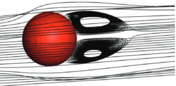
![Fig. 13. Illustration of streamlines for a flow past a sphere at Re = 250, on top our simulation and bottom corresponding results from [23]](https://thumb-eu.123doks.com/thumbv2/123doknet/3154932.89893/23.892.199.702.548.955/fig-illustration-streamlines-flow-sphere-simulation-corresponding-results.webp)
![Fig. 15. Characteristics of the final drop shape (from [14]).](https://thumb-eu.123doks.com/thumbv2/123doknet/3154932.89893/24.892.328.556.279.377/fig-characteristics-final-drop-shape.webp)
