an author's https://oatao.univ-toulouse.fr/27778
Jaroslawski, Thomas and Forte, Maxime and Delattre, Grégory and Gowree, Erwin Ricky and Moschetta, Jean-Marc Laminar to turbulent transition over a rotor at low reynolds numbers. (2021) In: 55th 3AF International Conference on Applied Aerodynamics, 12 April 2021 - 14 April 2021 (Piotiers, France).
55th 3AF International Conference
on Applied Aerodynamics. FP94-2020-jaroslawski
23 – 25 March 2020, Poitiers - France
LAMINAR TO TURBULENT TRANSITION OVER A ROTOR AT
LOW REYNOLDS NUMBERS
Thomas Jaroslawski (1) Maxime Forte(1) Gregory Delattre(1) Erwin Gowree(2) Jean-Marc Moschetta(2)
(1) ONERA, DMPE, Université de Toulouse, 31055, Toulouse, France. Email: [email protected]
(2) ISAE-SUPAERO, Université de Toulouse, 31055, Toulouse, France.
ABSTRACT
An experimental investigation on the flow topology and performance of a rotor operating at low Reynolds numbers is presented. The feasibility of laminar to turbulent transition experiments over small rotors is demonstrated. Phase-locked infrared thermography coupled with simultaneous force and torque measurements were used to study a three bladed NACA0012 rotor with a radius of 0.125 m and an angle of attack of 10 degrees. Boundary layer transition was fostered using two-dimensional (2D) and three-dimensional (3D) isolated roughness elements, placed at approximately 5% and 28% of the rotor blades chord. In the smooth rotor configuration, a 3D flow topology is observed, consisting of a clear laminar region closer to the blade root and a turbulent region at the blade tip. It was found that the state of the boundary layer can significantly affect the rotor’s performance, with the forcing of laminar to turbulent transition generally resulting in a loss of performance when compared to the smooth reference rotor case.
1. INTRODUCTION
Further knowledge of low Reynolds number flows is becoming increasingly important due to the rise in the demand of micro-aerial systems (MAS) and unmanned aerial systems (UAS). This encourages us to rethink the way conventional aerodynamic design is conducted, as these vehicles operate within a Reynolds number (Re= Vtipc / n ) regime of 103 < Re < 105 where one can expect
that the flow remains laminar to a greater extent but is still susceptible to transition. Understanding the impact of boundary layer transition becomes critical for the design of low Reynolds number flyers as it could lead to considerable deterioration in performance or in worst case scenarios, massive stall and control loss as they are more prone to separation in the low Reynolds number regime.
For 2D boundary layers subjected to a low disturbance environment, laminar to turbulent transition occurs through the exponential growth of Tollmien-Schichting (TS) waves. An adverse pressure gradient will
promote more rapid growth, reducing the local Reynolds number at which transition occurs. At low Reynolds numbers (<105) an LSB will be promoted in this recovery
or adverse pressure gradient region, significantly modifying the pressure distribution of the aerofoil. Environmental perturbations can be convected within the separation bubble and grow very rapidly leading to transition of the detached shear layer and reattachment to a turbulent state (Gaster 1967; Häggmark et al., 2000; Marxen et al., 2003a; Hosseinverdi and Fasel, 2019).
As mentioned above, the impact of the LSB and laminar separation on the performance of a 2D low Reynolds number aerofoil is well studied, however less is understood on how external perturbations such as roughness or freestream turbulence impact these mechanisms. Furthermore, for low Reynolds number rotors, there are significantly fewer studies. Singh and Ahmed (2013) took the LSB into consideration when designing a low Reynolds number wind turbine and noted that separation bubbles over low Reynolds number rotors cause excessive pressure drag, loss in aerodynamic lift and increase in the noise produced by the rotor. Koning et al. (2018) found little influence of the Mach number on the laminar-turbulent transition for low Re rotors. A recent study on the NASA Mars helicopter rover by Argus et al. (2020), used mid-fidelity RANS simulations coupled with a Blade Element Momentum Theory model to find that at Re= 20´103 and 80´103 increasing the
critical N-factor (an approximate measure of disturbance amplification to induce laminar to turbulent transition) from 3 to 11 decreased the figure of merit (FM) of the rotor by approximately 40%, suggesting that a performance gain is possible. They noted that in their configuration laminar separation without reattachment occurred.
Experimental investigations on boundary layer transition for rotor blades are relatively scarce. For example, some previous studies consisted of flow visualization with acenaphthene on full model scale rotors (Tanner and Yaggy 1966; McCroskey 1971). Contemporary boundary layer transition research on rotors commonly uses Infrared (IR) thermography, where
investigations on laminar to turbulent transition in rotary wing configurations entail more experimental difficulties than in fixed wing configurations. Richter and Schülein (2014) used high-speed IRT on boundary layer transition measurements on the suction side of a helicopter rotor. By synchronizing the IR camera with the rotor they were able to identify the start and end of transition by tracing the evolution of the pixel intensity for the entire rotor blade from a single IR image. Lang et al. (2015) used IRT and PIV to detect the presence of an LSB over a NACA 0015 rotor blade, showing that, the elevated temperature region could be used to determine the location of the bubble, the Re where the bubble was measured was 140´103. The locations of laminar separation and
turbulent reattachment were approximated through the analysis of the chordwise pixel intensity gradient. They defined the mean transition location as the mid-point between the location of laminar separation and turbulent reattachment. More recently, Thiessen and Schülein (2019) made a worthy experimental effort to understand the transition over a low Reynolds number rotor. They used IRT on a quadcopter rotor using laser heating. They suggest that there exists a region of separated flow, which they state to be an LSB that forms over the rotor blade, oil film topography measurements yielded further confirmation. The laminar separation bubble is a zone of almost stationary or low speed reverse flow, where the shear stress is zero or very low. In the separation region the heat transfer will be minimal and will begin to increase rapidly as transition and turbulent reattachment take place. In general, IR measurements conducted on a model which has a higher surface temperature than the free stream allows for identification of turbulent regions (low temperature), separated regions (high temperature) and laminar regions (medium temperature regions).
The objective of the present work is to demonstrate the feasibility of IR thermography to study boundary layer transition over small rotors at low Reynolds numbers and generate further insight into the 3D flow topology which will help in identifying the transition possible transition mechanisms.
2. METHODOLOGY 2.1. Experimental Setup
The experimental set up and test configurations are presented in Fig 1. The rotor had three blades with a NACA0012 profile, with a constant geometrical angle of attack of 10° and no twist. The radius (R) of the rotor was 0.125 m and the chord length (c) was 0.025 m, resulting the rotor having an aspect ratio (AR = R / c) of 5. Phase locked IRT was used to capture the temperature distribution of rotor blade surface. A Brüel & Kjær CCLD laser tacho probe was used to synchronize the blade with the IR Camera. A thin reflective film was placed on an opposing blade, so that for each rotation a voltage pulse was sent out by the laser to trigger the
camera. In order to increase the temperature difference between the ambient air and the blades surface, a 500W halogen lamp was used to heat-up the surface of the blade of interest. The experimental setup and test configurations are presented in Fig. 1.
Two chordwise positions for the roughness elements where used with the objective of investigating the impact of the roughness size with respect to the boundary layer thickness on transition. Where further downstream the boundary layer is expected to be thicker, resulting in the roughness element to have a smaller impact. The 2D roughness consisted of a carefully glued 100µm wire and the 3D roughness was comprised of adhesive laser pre-cut cylindrical discrete roughness elements spaced out at regular intervals, with a diameter of 1.27 mm, standard interval length of 2.54 mm and a of height of 200 µm. In total, one smooth and 8 roughness configurations at 6 different speeds where tested: the smooth rotor blade without any roughness is denoted as NoR, 2D roughness configurations are denoted as 2DR and 3D roughness configurations are denoted as 3D2SR, 3D3SR, 3D4SR for roughness spanwise spacing of 5.04, 7.62 and 10.16 mm, respectively. At the end of the abbreviation either P1 or P2 is used to indicate the chordwise position of the roughness element, where P1 and P2 indicate 0.05c and 0.28c, respectively. The rotational speed, Ω, was varied from 1000 to 6500 RPM, yielding a Reynolds number range of 6.2´103 to 144´103 based on radial speed,
Figure 1. Experimental setup and test configurations The presumption of laminar to turbulent transition via IRT is based on the principle that laminar and turbulent flows have different heat transfer rates, where turbulent flows tend to have a higher rate of heat transfer between the bulk fluid flow and the wall, due to a higher value of skin friction, 𝑐!. By means of the Reynolds
assumption (Richter and Shülein 2014), the Stanton number illustrates this behavior and is defined in Eq. 1 , where ℎ denotes the heat transfer coefficient, 𝜌 is the fluid density, 𝑈" is the flow velocity and 𝑐# is the
pressure coefficient. 𝑆𝑡 = ℎ 𝜌𝑐𝑝𝑈∞ ~ 𝑐𝑓 2 (1) During the IR camera measurement the heating lamp was turned off, the motivation of this technique is that in a turbulent flow region there will be more heat transfer between the wall and outer flow than in a laminar flow region. Therefore the temperature (pixel intensity) will vary differently in a turbulent, laminar or separated region as a function of time. Since a variety of configurations were tested, a pixel intensity normalization technique needed to be implemented for coherent analysis. Each IR image was normalized by the maximum pixel intensity present in the image so that the different test configurations would compared reliably.
Before starting the IR measurement, the blade of interest was systematically heated by the lamp at a distance of 0.15 m for 10 seconds. The room temperature was at 20 °C and the blade was heated to approximately 35-40 °C in each case, however the absolute temperature is not of great importance as the transition detection techniques are based on temperature differences. The Richardson number can be used to address the extent of the relevance of natural convection to forced convection. The Richardson number is defined in Eq. 2, where 𝜃, represents the volumetric thermal expansion coefficient. The model wall temperature, a denotes the rotational acceleration ( a = 𝑈𝑡𝑖𝑝2 / r ), and the ambient air
temperature are denoted by 𝑇𝑤 and 𝑇∞, respectively.
𝑅𝑖 = 𝑎𝜃𝑐(𝑇𝑤− 𝑇∞)/𝑈𝑡𝑖𝑝2 , (2)
Natural convection can be considered to be negligible if Ri < 0.1, in the present work Ri ~ 0.0032 at
r / R = 0.1 and decreases as r/R is increased, therefore
natural convection effects on the flow can be neglected. The high speed and high resolution IR camera (Telops Fast M3k) was used to characterize the flow topology of the rotor, where the pixel intensity is used to approximate the state of the boundary layer. The camera had 320 x 256 pixel spatial resolution, a typical Noise Equivalent Temperature Difference (NETD) of 25 mK
and operated in the 1.5 – 5.4 µm spectral range and was positioned 0.4m away from the rotor blade. The size of the field of view was 1c x 0.65R and the exposure time of the camera was 71µs, allowing for a good compromise between camera noise and motion blur. Since the camera was synchronized with the rotor, effectively, the sampling rate was that of the rotors turning rate (RPM) for the given run. There were at least 500 phase locked images captured for each run.
3. RESULTS
The following section presents the results of the force and torque measurements followed by the results of the IR measurements for both untripped (smooth) and tripped (2D and 3D roughness) configurations.
3.1. Force Measurements
Thrust and torque measurements were conducted simultaneously with IR camera measurements. The Figure of Merit (FM) and Power Loading (PL) are defined in Eqs. 3 and 4, Where T is the thrust, Q is the torque, r is the density of the ambient air, Ω is the rotational frequency and R is the rotor blade radius. The objective of these measurements was not to find an optimal tripping configuration, rather to demonstrate that the state of the boundary layer on a rotor operating at low Reynolds number can significantly affect the performance.
𝐹𝑀 = 𝑇3/2/ Ω𝑄√2𝜋𝑅2 (3)
𝑃𝐿 = 𝑇 / Ω𝑄 (4)
Referring to Figs. 2 an 3., the FM and PL are presented. It is interesting to note that more tightly spaced roughness
configurations perform worse than roughness
configurations which were further apart. This signifies that the interaction and spreading of the wakes downstream of the roughness plays a significant role in the transition process and performance of the rotor. The present results show that at lower Reynolds numbers and RPM, the effects of roughness are more prominent and that forcing transition generally results in a decrease in performance both in terms of FM and PL. The roughness height was not optimized in the present work, as a result
there are regions on the rotor where the boundary layer that are “over tripped”, resulting in massive performance loss. At the higher RPM and Re, the displacement thickness (approximately 2-3 times smaller than 𝛿, indicating that the roughness has a height beyond the critical height.) is smaller than the roughness element. The chordwise position of the roughness elements has a significant impact on the rotor performance.
Figure 2. Figure of Merit for all tested roughness configurations (top: tripping at 5% chord, bottom
boundary layer tripping at 28% chord).
Figure 3. Power Loading (PL) for all tested roughness configurations (top: tripping at 5% chord, bottom boundary layer tripping at 28% chord).
3.2. IR Measurements
In this section the results of the IR thermography measurements are presented. The smooth rotor configuration is presented in 3.2.1 and the configurations with boundary layer tripping are presented in 3.2.2 and 3.2.3.
3.2.1 Smooth configuration
The time averaged IR measurements of the clean, NoR configuration are presented in Fig. 4. For the three different rotational speeds the 3D nature of the flow is clear, where the spanwise (radial) non-uniformity is accentuated with increasing rotational speed.
Due to the experimental difficulty in measuring the boundary layer thickness (𝛿) over a rotating surface, the 𝛿 was calculated using ONERA’s in house boundary layer code 3C3D. The coefficient of pressure (Cp) over
the suction side of the rotor aerofoil was calculated using XFOIL. The local angle of attack was approximated with Blade Element Momentum Theory (BEMT) for the Reynolds number range investigated. The approximation of the range the values of 𝛿 are presented in Table 1.
Table 1. Estimated boundary layer thickness (in mm) near the rotor blade root (r/R = 0.3) and rotor blade tip (r/R = 1) and corresponding Reynolds numbers for 1000, 3000 and 6500 RPM.
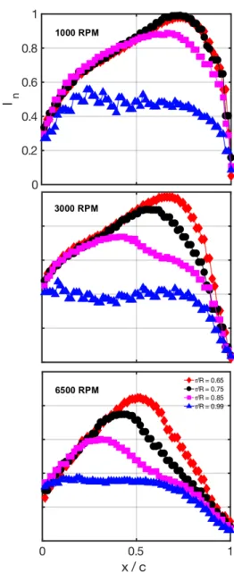
Referring to Fig 5, the location where 𝜕𝐼$ / 𝜕x ~
0 corresponds to where the skin friction is zero (Richter and Schülein 2014). The chordwise evolution of the pixel intensity is essentially the Stanton Number. The maxima in pixel intensity should indicate the region with low momentum similar to that in a separation bubble and rapid change in pixel intensity downstream would be due to high mixing turbulent flow. Therefore, here the location where 𝜕𝐼$ / 𝜕x ~ 0, the minimal value in skin
friction can be considered as the end of the transition process (if similarity was to be drawn with laminar separation bubble) and the point where a turbulent reattachment occurs.
On a heated surface, IR thermography measurements would show that a separated region of flow will cool down at a rate much slower than an attached flow. The same is true for an LSB, the region of almost stationary or low momentum flow will undergo very slow temperature change compared to an attached laminar or turbulent flow with the rate of change in the latter being greater. Referring to Fig. 6, the normalized pixel intensity ( 𝐼$, temperature higher with increasing
𝐼$) was probed at six positions along the span of the rotor,
with P1- P3 located in a region where the flow is suspected to be turbulent and P4 - P6 could be in a region of low momentum flow in the chordwise direction as in an LSB or laminar separation, which aggress with the rationale used by Miozzi et al. (2019), Thiessen and Schülein (2019), Wynnychuck and Yarusevych (2019) From the temporal pixel intensity evolution presented in Fig. 6 the difference between the inboard and the outboard station shows a variation of pixel intensity, which in turn, could imply a variation in the state of the flow.
Figure 5. Chordwise evolution of IN for radial positions
of r/R = 0.65, 0.75, 0.85, 0.99 for rotational speeds of 1000, 3000 and 6500 RPM.
In the regions of P4, P5 and P6 the evolution of 𝐼$ remains relatively constant confirming the presence of
a low momentum region, compared to positions P1, P2 and P3 where 𝐼$ decays rapidly due to higher mixing
possibly indicating the presence of a turbulent flow. Similar behaviour of low Reynolds number flows was demonstrated via IRT and PIV measurements by Lang et al. 2015 over a rotor and Miozzi et al. (2019) over a fixed aerofoil, both operating in a similar Reynolds number range as in the present work. Even if the low momentum regions (P1, P2 and P3) show similar behaviour in terms of rate of temperature change the flow is expected to behave rather differently from a laminar recirculating bubble over an upswept or 2D wing, where it retains spanwise uniformity. Ω Re ´103 (r/R =0.3) Re´103 (r/R =1) !!.!#$ (r/R =0.3) !!.!#$ (r/R =1) !!.%&$ (r/R =0.3) !!.%&$ (r/R =1) 1000 6.2 22 0.321 0.204 1.102 1.081 3000 19 66 0.182 0.131 0.633 0.615 6500 40 144 0.128 0.089 0.435 0.344
Figure. 6 Top: IR measurements of NACA 0012 (NoR configuration) rotor at 3000 rpm; Bottom: The differential temporal decay (𝐼$− 𝐼$%) of the normalized
pixel intensity (cooling) in a region of relatively stagnant temperature (P4-P6) and a region of rapid decay (P1-P3). The time axis (x) is normalized by tip velocity (Vtip) and
aerofoil chord.
3.2.2 2D Roughness configuration
The time averaged IR images of the 2D roughness configurations are presented in Fig. 7, with blue lines denoting the location of the 100µm trip. One of the major effects of the upstream 2D boundary layer trip is that the flow topology becomes more uniform in span (2D) compared to the untripped case, where a clear spanwisely varying (3D) flow topology was observed (refer to Fig 4.). Additionally, when the boundary layer trip is moved downstream, to a position of 0.28c, we can see that the pixel intensity abruptly decreases downstream of the wire, which suggests that the flow could transition in this region. This is due to the fact that the boundary layer would be thicker at 0.28c than at 0.05c, therefore the wire could provide a smaller disturbance in the boundary layer. As the Reynolds number increases, region of low pixel intensity moves upstream, signifying that the transition position in the 2DRP2 configuration moves closer to the wire which is expected as the boundary layer would be less stable. A similar observation can be made for the 2DRP1 configurations, where at 1000 RPM the flow topology remains similar to that on the clean aerofoil case indicating that the trip was not effective in tripping the boundary layer compared to 6500 RPM where the flow
appears to have been impacted by the presence of the wire and is possibly turbulent over most of the rotor blade (refer to Fig. 7).
Figure 7. IRT measurements of the 2D roughness configurations, where the blue line represents the tripping location. Top: 2DRP1; Bottom: 2DRP2
3.2.3 3D Roughness configurations
The IR measurements for the 3D roughness configurations at 5% and 28% are presented in Figs 8-10. We observe the formation of turbulent wakes and wedges behind the roughness elements.
Once the critical roughness Reynolds number is attained the streaks downstream of the isolated roughness break down into turbulent wedges as observed during very early experiments of Gregory and Walker (1956), where at larger roughness Reynolds numbers the breakdown could occur immediately downstream of the
roughness element. In the majority of cases tested, turbulent wedges are observed right after the roughness element and is explained by the fact the roughness elements are close to the height of the approximated boundary layer (Refer to Table 1.).
The wedge angle increases gradually as the rotation speed increases and the more extreme angles occur near the rotor blade tip, which could be larger due to blade tip vortices contaminating the turbulent wedge. At lower Reynolds numbers, the streaks might not breakdown at all (as seen at low RPMs in the present case), by increasing the Reynolds number, the streaks breakdown earlier and the wedge moves upstream, closer to the roughness, a further increase in the Reynolds number will promote immediate breakdown.
Finally, referring to Figs. 8-10, slight radial tilting of the undeveloped wakes generated by the roughness elements is observed. This could be due to the spanwise flow generated by the pressure gradient or rotational forces. As the radial position increases the radial tilting decreases and the wakes breakdown into turbulent wedges.
Figure 8. IRT measurements of the 3D roughness high packing density configurations. Top: 3DR2SP1; Bottom: 3DR2SP2
Figure 9. IRT measurements of the 3D roughness high packing density configurations. Top: 3DR3SP1; Bottom: 3DR3SP2
Figure 10. IRT measurements of the 3D roughness high packing density configurations. Top: 3DR4SP1; Bottom: 3DR4SP2
4. DISCUSSION
Tripping the boundary layer with roughness demonstrated a significant performance loss, however it is important to note that the roughness height was not
optimized in the present work, resulting in the boundary layer being “over tripped”. As mentioned in the results section, there could be a separated region of flow over the rotor and the addition of the optimal roughness could improve the performance. Systematic investigations on the impact of boundary layer trip height on rotor performance are warranted. The FM and PL increase when the roughness elements are moved from 0.05c to 0.28c. This is explained by the fact that the boundary layer thickness increases as the flow moves downstream. For example, at 3000 RPM, 𝛿𝟎.𝟎𝟓𝒄 = 0.131 mm and 𝛿𝟎.𝟐𝟖𝒄
= 0.633 mm, the 2D wire (0.1mm thick) and 3D isolated roughness elements (0.2 mm) will indeed provide a smaller perturbation to the boundary layer, resulting in transition occurring further downstream of the roughness element. At lower values of RPM and Reynolds number, where the roughness height is approximately 5 times smaller than the boundary thickness, the FM is unaffected by the presence of the roughness.
The impact of boundary layer transition on helicopter rotors (larger Re ~ 106) performance is known
to be detrimental. For example, Overmeyer and Martin 2017 investigated the impact of the boundary layer transition on a Mach scaled helicopter rotor. They found that when the transition was forced using roughness elements (placed at 0.05c) the FM decreased significantly. Richez et al. 2017 demonstrated that selecting the correct transition model in numerical simulations over a helicopter blade is critical to reproducing experimental data.
Experimental studies on the effects of roughness on transition for low Reynolds (Re = 104 – 105) number
rotor are scarce, therefore it is difficult to compare results to previous work. However, recent simulations on the NASA Mars rotor (Argus et al. 2020) showed that at lower Reynolds numbers configurations (Re< 100E3) the thrust generated by the rotor was slightly larger when transition occurred earlier (smaller critical N-factor) compared to when transition occurred later (larger critical N-factor). They suggested that earlier transition could eliminate boundary layer separation, resulting in a performance gain. At higher Re the benefit of early transition diminished and became detrimental for the thrust produced by the rotor. A similar trend was observed in the FM, where increasing critical N-Factors from 3 to 11 decreased the FM of the rotor by approximately 40%. This contradicts the present results,
however, we must state, that the rotor studied in Argus et al. (2020) had a much larger AR and transition was induced by decreasing the N-factor, meaning that the transition mechanism was different to the current work, where modal transition is bypassed with the roughness element.
In addition to the impact on performance, tripping the boundary layer with different roughness configurations significantly changes the flow topology over the surface of the rotor. In the case where the boundary layer is tripped via 3D roughness, possible tilting of the wakes downstream of the roughness elements is present, especially when they were yet to develop into turbulent wedges. From our measurements we observe that when the roughness Reynolds number, ,𝑅𝑒, (based on roughness height and the local tangential
velocity component, Vlocal = Ωr) is larger than
approximately 40 the turbulent wedge will develop, below this value the wakes generated by the roughness elements did not undergo break down. Previous work by Braslow (1960), demonstrated roughness could induce transition when ,𝑅𝑒, was approximately 20 – 30,
therefore the current results are not surprising.
When the roughness elements are located at 0.28c the turbulent wedges also formed ,𝑅𝑒, ≈
40 however they appear further downstream of the roughness element compared to the 0.05c configurations, due to the fact that the boundary layer is thicker at this position (refer to Table 1). Between the turbulent wedges and further downstream, the pixel intensity continues to increase and reaches a similar pixel intensity as in the wedge, which could allow for natural boundary transition to occur as observed in Richer and Schülein (2014). As the spacing between the roughness elements decreases the flow transitions further upstream due to the turbulent wedges interacting with each other.
The flow topology measurements show that the type of tripping 2D or 3D can modify the transition front significantly. According to 2D modal stability theory a critical 3D roughness will introduce a larger perturbation to the boundary layer as opposed to an equivalent 2D roughness. But here we observed that despite being twice lower in height the 2D roughness was more efficient in tripping the flow than the 3D roughness.
The slight radial tilting of the undeveloped wakes (Refer to Figs. 8-10) could be caused by a spanwise flow over the rotor, which will be generated by the pressure gradient or rotational forces, or a combination of both. In the present case, since there is no approach velocity AR = Ro, where the Rossby number is a dimensionless parameter to measure the relative contribution of the convective flow acceleration to Coriolis and centrifugal acceleration. Therefore, for a rotor with AR = 5, the rotational forces should be in the same order of magnitude as the convective forces. Weiss, et al. 2019 found that when the local AR is 4.76, there are no effects
of rotational forces on the boundary layer transition or chordwise extent of laminar flow over a DSA-9A aerofoil rotor. Numerical simulations by Hernandez (2012) over a NACA0015 rotor showed that rotational forces can have a stabilizing effect on boundary transition when Ro tended towards 1.
5. CONCLUSION
The performance and flow topology of a three bladed NACA 0012 rotor was investigated using IR thermography with simultaneous force and torque measurements to address the knowledge gap of the impact of laminar to turbulent transition on rotors operating in the low Reynolds number range of 103 to
105.
It was demonstrated that the state of the boundary layer has a significant effect on the performance of the rotor. Forcing laminar to turbulent transition with roughness results in a significant decrease in FM and PL. Roughness configurations with tight packing resulted in the largest performance losses and more sparse configurations where found to have almost the same performance as in the smooth reference case at lower RPM.
A 3D flow topology is observed, where a 3D separated region of flow is suspected based on the evolution of the temperature following that of Cf
distribution for a separated flow. However the existence of this 3D separated region cannot be exclusively confirmed from the present measurements.
Even if transition is seen to have a detrimental effect in this non-optimized rotor configuration, during multi-physics optimisation a compromise with aero-acoustic or aeroelastic performance could be achieved through boundary layer tripping. Therefore an understanding of the unperturbed flow topology becomes necessary for the placement of the optimal boundary layer trip.
Finally, the feasibility of conducting boundary layer transition experiments on a small rotor (radius of 12.5 cm, AR = 5) operating at low Reynolds numbers (103
-105) was demonstrated.
6. REFERENCES
[1] M. Gaster, “The Structure and Behaviour of Laminar Separation Bubbles,” Aeronaut. Res.
Counc. Reports Memo., no. 3595, pp. 1–31,
1967.
[2] C. P. Häggmark, A. A. Bakchinov, and P. H. Alfredsson, “Experiments on a
two--dimensional laminar separation bubble,” Philos.
Trans. R. Soc. London. Ser. A Math. Phys. Eng. Sci., vol. 358, no. 1777, pp. 3193–3205, 2000.
[3] O. Marxen, M. Lang, U. Rist, and S. Wagner, “A combined experimental/numerical study of unsteady phenomena in a laminar separation bubble,” Flow, Turbul. Combust., vol. 71, no.
1–4, pp. 133–146, 2003.
[4] S. Hosseinverdi and H. F. Fasel, “Numerical investigation of laminar--turbulent transition in laminar separation bubbles: the effect of free-stream turbulence,” J. Fluid Mech., vol. 858, pp. 714–759, 2019.
[5] R. K. Singh and M. R. Ahmed, “Blade design and performance testing of a small wind turbine rotor for low wind speed applications,” Renew.
Energy, vol. 50, pp. 812–819, 2013.
[6] W. J. F. Koning, E. A. Romander, and W. Johnson, “Low reynolds number airfoil evaluation for the mars helicopter rotor,” Annu.
Forum Proc. - AHS Int., vol. 2018-May, pp. 1–
17, 2018.
[7] F. J. Argus, G. A. Ament, and W. J. F. Koning, “The Influence of Laminar-Turbulent Transition on Rotor Performance at Low Reynolds
Numbers,” 2020.
[8] W. H. Tanner and P. F. Yaggy, “Experimental boundary layer study on hovering rotors,” J.
Am. Helicopter Soc., vol. 11, no. 3, pp. 22–37,
1966.
[9] W. J. McCroskey, Measurements of boundary
layer transition, separation and streamline direction on rotating blades, vol. 6321. National
Aeronautics and Space Administration, 1971. [10] K. Richter and E. Schülein, “Boundary-layer
transition measurements on hovering helicopter rotors by infrared thermography,” Exp. Fluids, vol. 55, no. 7, 2014, doi: 10.1007/s00348-014-1755-z.
[11] W. Lang, A. D. Gardner, S. Mariappan, C. Klein, and M. Raffel, “Boundary-layer transition on a rotor blade measured by temperature-sensitive paint, thermal imaging and image derotation,” Exp. Fluids, vol. 56, no. 6, pp. 1–14, 2015, doi: 10.1007/s00348-015-1988-5.
[12] R. Thiessen and E. Schülein, “Infrared Thermography and DIT of Quadcopter Rotor Blades Using Laser Heating,” in
Multidisciplinary Digital Publishing Institute Proceedings, 2019, vol. 27, no. 1, p. 31.
[13] M. Miozzi, A. Capone, M. Costantini, L. Fratto, C. Klein, and F. Di Felice, “Skin friction and coherent structures within a laminar separation bubble,” Exp. Fluids, vol. 60, no. 1, p. 13, 2019. [14] N. T. Gregory and W. S. Walker, The effect on
transition of isolated surface excrescences in the boundary layer. HM Stationery Office,
1956.
[15] A. D. Overmeyer and P. B. Martin, “Measured boundary layer transition and rotor hover performance at model scale,” in 55th AIAA
Aerospace Sciences Meeting, 2017, p. 1872.
[16] F. Richez, A. Nazarians, and C. Lienard,
“Assessment of laminar-turbulent transition modeling methods for the prediction of helicopter rotor performance,” in rd European
Rotorcraft Forum (), 2017.
[17] A. Weiss, A. D. Gardner, T. Schwermer, C. Klein, and M. Raffel, “On the effect of rotational forces on rotor blade boundary-layer transition,” AIAA J., vol. 57, no. 1, pp. 252–266, 2019.
[18] S. J. N. & S. W. Z. Martinez Hernandez G. G., “Laminar-Turbulent transition on Wind