AUTOMATIC 3D BUILDINGS COMPACT RECONSTRUCTION FROM LIDAR POINT
CLOUDS
G.-A. Nys 1,*, R. Billen 1, F. Poux 1
1 Geomatics Unit, University of Liège (ULiège), Allée du six Août, 19, 4000 Liège, Belgium; (ganys, fpoux, rbillen)@uliege.be
Technical Commission TCII - Photogrammetry
KEY WORDS: LiDAR, Smart Cities, 3D City Model, CityJSON, Point Cloud
ABSTRACT:
Point clouds generated from aerial LiDAR and photogrammetric techniques are great ways to obtain valuable spatial insights over large scale. However, their nature hinders the direct extraction and sharing of underlying information. The generation of consistent large-scale 3D city models from this real-world data is a major challenge. Specifically, the integration in workflows usable by decision-making scenarios demands that the data is structured, rich and exchangeable. CityGML permits new advances in terms of interoperable endeavour to use city models in a collaborative way. Efforts have led to render good-looking digital twins of cities but few of them take into account their potential use in finite elements simulations (wind, floods, heat radiation model, etc.). In this paper, we target the automatic reconstruction of consistent 3D city buildings highlighting closed solids, coherent surface junctions, perfect snapping of vertices, etc. It specifically investigates the topological and geometrical consistency of generated models from aerial LiDAR point cloud, formatted following the CityJSON specifications. These models are then usable to store relevant information and provides geometries usable within complex computations such as computational fluid dynamics, free of local inconsistencies (e.g. holes and unclosed solids).
*Corresponding author
1. INTRODUCTION
The digital twins are part of a movement that focuses attention on collaborative processes. These replicas allows a better understanding of the urban built environment and in particular the management of flows (winds, floods, heat radiation, etc.). It is not only a common representation of a city but an integrating base for all applications and usages. It aims to improve cities assets management: traffic, environmental monitoring, calorific diagnosis, etc. Hence, the stakeholders’ collaboration in a single digital model could improve their insight taking into account an increased number of factors. Beside these urban-centred considerations, the pooling and the sharing of knowledge are part of a dynamic increasingly focused on the web. Formatting the data in a normalised way allows its exchange in a collaborative way. CityJSON, as a lightweight version of the CityGML schema, provides a structure to represent cities following the new web trends and formats. In this research, we target the automatic reconstruction of consistent 3D city buildings highlighting closed solids, coherent surface junctions, perfect snapping of vertices, etc. Within the urban context, the automatic generation of buildings, i.e. the city backbone, from an airborne laser scan (ALS) is the first step in an integrated solution for the smart cities management.
Guiding this transformation, this paper is structured as follows: first, the advantages of JSON-encoding are presented in regard of the XML format specifications. CityJSON is presented and discussed on the main lines. In a second time, the segmentation of the scattered point cloud is made thanks to unsupervised methods. Two methods have been tested: RANSAC shape detection and region growing based on curvature smoothness. From the segmented parts, the roof planes and their
corresponding connectivity graph are constructed. Roof vertices and rupture elements are then generated under the strict condition of perfect snapping (i.e. no holes are allowed). After this, before moving to conclusion and future works, the results are discussed taking into account the topologic and geometric consistency of the generated models. Official tools as CJIO and val3dity ensure the quality control.
2. RELATED WORKS
Generating buildings from airborne point cloud is now a common procedure. In general, modelling building rooftops from ALS data can be categorized into data-driven, model-driven and hybrid-model-driven (Wang et al., 2018). Our methodology is part of the graph-based modelling. It is a subpart of the hybrid-driven family, since it is based on the Roof Topology Graph (Verma et al., 2006). It is a good balance between the flexibility of the reconstruction methods and the quality of the reconstructed building models. Among others, several researches propose solutions similar to the RT graph: Roof Attribute Graph (RAG) (Hu et al., 2018) or the Roof Topology Graph (Xiong et al., 2015). The main difference with these graphs lies in the parallelism support: the other proposals do not consider parallelism in its own right. Considering it, the provided simplification allows a more efficient management of gable roofs among others. It is especially useful in Belgium where gable roofs represent the majority of roof shapes. Some differences with other recent works are notable: CityJSON is not yet considered; generation steps are not always in the same order; primitives modelling tend to fit premade models to point clouds reducing metrics (RMSE, Hausdorff distance, etc.) (Wichmann, 2018). Commonly, no matter the construction method, not all models are relevant in The International Archives of the Photogrammetry, Remote Sensing and Spatial Information Sciences, Volume XLIII-B2-2020, 2020
order to perform complex processes: finite elements computations suffer from non-coherent geometries and local singularities (i.e. the slightest hole can lead to aberrant results). Therefore, the topological consistency of the generated geometries is a major concern. The methodology is similar to the one proposed in TopoLAP (Liu et al., 2019). Even if the topology of planar and linear primitives is the primary purpose of this process also, the compactness of the models could limit their usability in small devices. Moreover, airborne data are used for the registration of models but the generation of the models impose the use of photogrammetry. On the other hand, about the accuracy of the generated roof planes, improvements are made with more or less results adjusting the models iteratively (Kurdi et al., 2019). Note that the standard deviation of lower quality is justified by the low accuracy of the point cloud (acquired in 2002 and 2008 - point density varying between 4 and 9 point per square meter).
3. 3D CITY MODELS
The JavaScript Object Notation (JSON) data specifications allow developers to store and transmit information in a human-readable format. It is an effective syntactic framework for data interchange. Moreover, on the other side, machines can efficiently parse and generate it. It is often adopted in mobile and web-based applications since it is light and compact. In the context of 3D City modelling, CityJSON proposes a compact and easy-to-use JSON-encoding for semantic 3D city models (Ledoux et al., 2019). It is maintained by the 3D Geoinformation of the TU Delft. Its 1.0.x version follows the CityGML 2.0 conceptual model and focuses, among others, on reducing the number of redundancies (Gröger & Plümer, 2012). In this research, the generated city models concentrate compactness, expressivity and interoperability using the promising CityJSON format.
In more detail, JSON is less verbose and faster than XML: it does not use end tags, which reduce format redundancies; it uses arrays, which do not impose to repeat metadata; etc. Nonetheless, several points agree on their usability, as they are both self-describing, hierarchical and fetched within HTTP requests. About the hierarchy in particular, while JSON is structured as a map (similar to nested key-value pairs), XML is structured as a tree. Trees can be tedious and time-consuming task to parse. Hence, in short, XML is better to store information, thanks to namespaces, and JSON is for data delivery, thanks to its compactness.
Previous works have proposed pipelines to create approximate CityGML models and use them in diverse applications (Billen et al., 2014; Biljecki et al., 2015). However, as the use of city models are expanding in many web-based applications and thus mobile devices, CityJSON should find a place in this ecosystem by offering a light alternative. Note that CityJSON is currently in discussion to become an OGC Community Standard.
4. METHODOLOGY
In order to be agnostic from the input source, we use only X, Y, and Z attributes from point cloud data. No symmetry, global regularity or repetition rules are set up. Only the intrinsic information brought by the points coordinates are used. The test data are those produced by the Walloon Public Service
over the south part of Belgium. Those have been acquired during the summer of 2012. It represents a mean point density of 0.78 point per square meter, which defines it as a sparse point cloud.
The methodology reconstructs objects in a level of details that represents roof shapes under refined conditions (LoD 2.x) (Biljecki et al., 2016). It is here worth mentioning that if LoD 2.x could not be generated for an object, we still generate LoD 0.x and LoD 1.x. As these levels are easier to generate and could overvalue the accuracy, the accuracy study in the end of this paper does not consider these geometries in the synthesis. The height of the LoD 1.x elements is the maximum height of the points (i.e. LoD 1.x is the bounding box of the building). The approach is subdivided in four consecutive steps: (a) unsupervised point cloud segmentation to detect roof planes; (b) construction of connectivity graph and the corresponding roof shape; (c) generation and semantic labelling of planes (“GroundSurface”, “RoofSurface” and “WallSurface”) and (d) reconstruction of the 3D CityJSON buildings and city model. Some metadata are computed and are added to the model afterwards (e.g. the global bounding box). Several elements of related works, which bring an improvement to a specific step, are discussed in the following section.
4.1 Segmentation
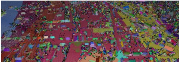
The correct detection of planar surfaces is essential and represents a basic assumption in the succession of the different modules. Two unsupervised segmentation algorithms and some refinements have been compared: RANdom SAmple Consensus (RANSAC) for shape detection and region growing based on curvature smoothness. The preliminary results of the fully unsupervised region-growing algorithm is shown in Figure 1. The choice of these algorithms was motivated by their robustness concerning outliers, their effectiveness to infer planar shapes (i.e. roof segments) and the minimal tuning of hyper-parameters. The implemented region growing algorithm, even if it has been developed for indoor purposes, shows very promising results in the urban built environment (Poux et al., 2018). This is an interesting intermediate result since the nature of airborne LiDAR data is much sparser than indoor point clouds. Potential improvements could study the tuning of parameters on curvature and point density to improve the element detection.
Figure 1. Fully unsupervised segmentation's results In both methods, RANSAC is used to interpolate planes on points clusters rather than least mean squares (Schnabel et al., 2007). Differences between the two are listed below: (a) the first method only relies on RANSAC to determine the maximum number of planes following a short list of parameters (distance to be considered as an outlier and minimum number of points to form a plane). The algorithm then randomly determine seeds and aggregate points as they The International Archives of the Photogrammetry, Remote Sensing and Spatial Information Sciences, Volume XLIII-B2-2020, 2020
meet the cluster requirements. Method B does not rely on any hyper-parameters but determines clusters of points based on their common intrinsic or assimilated attributes. (b) RANSAC is often seen as a limiting process because it is time-consuming. This is checked one more time here as the whole process is 58% longer in the first method where RANSAC identifies planes without any previous segmentation. On the other hand, the region growing method processes one million of points in a second. Nonetheless, the errors are located on the same buildings. This point informs us that the point cloud is most certainly locally problematic (too sparse, cluttered, etc.). Overall, the final quality of buildings is not far different between the two methods.
4.2 Roof construction
Once point’s clusters are segmented, planes are interpolated using RANSAC by extracting the point’s normal and their respective inliers. From these characteristics, the spatial extent of each plane is determined by determining the minimum oriented bounding rectangle comprising the inliers. Then, the assemblage of different planar primitives is conducted by constructing the connectivity graph (Verma et al., 2006). The planes relationship can be classified within three constrained families and a default one:
• O+ planes have normals that when projected are orthogonal and point away from each other.
• O- planes have normals that when projected are orthogonal and point towards each other.
• S+ planes have normals that when projected are parallel and point away from each other.
• N no constraint.
This normalised graph collects the connectivity information between the planar segments but also the nature of these connections (valleys, hips and ridges). The information about the topology between the planes is defined according to the distances of the planes and their overlap. Point out that the N family is not stored at all as it does not bring any information. Since elements are connected in pair, the connectivity and its nature are sorted in two matrices: adjacency (arrays of connected elements) and relationship (nature of the adjacency). In order to refine the grouping, the connections are translated into “rupture elements”. These elements define connection modes between pair of planes. For instance, the parallel roof planes of a gable roof are intersected as a rupture line and two points intersects the roof perimeter. The line and these points are parts of the backbone of the roof shape. From these sets of “rupture elements” and the connectivity graph, the roof shape is geometrically constructed linking vertices and lines of all pairs. In order to ensure an accurate and coherent representation of buildings, a perfect snapping tolerance of vertices is essential for the generated model. In the case where a vertex belongs to several planes (commonly two or more), its height is computed as the mean between the planes equations to which it belongs. This allows spreading the error in a manner that reduces its relative impact on planes interpolation. Finally, by projecting the detected planes on the digital elevation model (sub-product of the LiDAR campaign), we can determine the footprint of the building. Note that the generalisation of this footprint is made under normalised
CityGML specifications (e.g. the footprint of a building should be greater than six square meters wide). In the end, what comes out of this module are the footprint of the building and several roof planes suspended right over it.
4.3 Labelling planes
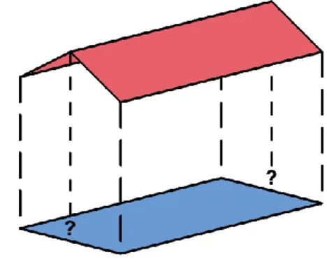
The semantic labelling of the planes are direct and unequivocally. Only three classes are encountered during the process: “RoofSurfaces”, “GroudSurfaces” and “WallSurfaces”. Since roof planes are always determinate in first and footprint comes in a second time, there is no space left for semantic uncertainty. Afterwards, the walls are generated as linking components of the two previous sets. It is by travelling through the successive edges of the footprint that we find the homologous edges from the roof planes. Note that this automatic mapping is not straightforward since not all roof vertices have homologous vertices in the footprint. It is especially the case in gable roofs where roof backbone directly connects to the periphery elements but none remarkable element of the footprint corresponds to it (see Figure 2). To ensure the consistency of the wall surfaces, the non-intersecting polygon is determinate based on the intersection of vertices from the roof projected on the XY plane and the footprint segment. The wall surfaces are consequently considered as vertical.
Figure 2. Closing of the geometry by the walls It is here worth mentioning that the normal direction of surfaces do have an important impact, sometimes for the semantic validity of the model, sometimes for visualisation purposes. Once the building geometry has been determinate, one can validate that normals are pointing towards the exterior of the building. Otherwise, if back-face culling is a consideration, models can be non-coherent in some applications.
4.4 Construction of buildings and city models
The proposed methodology partially relies on the binding hypothesis that the segmentation properly detects planes and their related connectivity graph. In the case when a plane is not consistent or correctly segmented, it is simply not generated. Therefore, some geometries lack of some planes but the rest of the whole geometries is still created. Improvements can close failing geometries: one can for instance use a top-down shrink-wrapping process to remesh the polygonal surfaces (Zhao et al., 2013).
The International Archives of the Photogrammetry, Remote Sensing and Spatial Information Sciences, Volume XLIII-B2-2020, 2020 XXIV ISPRS Congress (2020 edition)
Once the footprint, the roof planes and the walls are generated, the buildings are reconstructed following the 1.0.1 CityJSON specifications. The city model consists of the concatenation of all the buildings as Solids geometries (See Figure 3). Metadata complete it all providing information about the coordinate reference system, the geographical extent of the model, the model versioning, etc.
Figure 3. Generated city model 5. RESULTS
On a visual basis, the generated city models look promising. Even if some geometries are inconsistent or incomplete, they represent a reduce part of the whole (See bottom right of the Figure 3). Even if gable roof shapes represent the majority of the roofs shapes, pyramidal and more complex shapes are represented within the dataset also. The consistency of models is studied on two different aspects: format compliance and topological/geometrical consistency. While the first is made overall on CityJSON compliance of the generated file, the second is guaranteed during the process on buildings parts and buildings. The conformity at every level is assessed with official tools afterwards.
Concerning the CityJSON compliance, the format is controlled thanks to the Python Command Line Interface CityJSON/io (https://github.com/cityjson/cjio). No error is encountered at all for vertex indices coherency, specifics for CityGroups, semantic arrays coherency with geometry, root properties, empty geometries, duplicate vertices, orphan vertices and required CityGML attributes. It is mainly explained by the fact that every single attribute is restrained during the process: metadata are simple; semantic uncertainty is handled in the different modules; JSON-encoding is intuitive, etc.
As stated before, when it comes to use the city models in simulations such as Computational Fluid Dynamics (i.e. wind, floods, etc.), the geometric coherence and integrity to common topological rules are primordial. This restrictive hypothesis imposes to produce sometimes models at the expense of a certain misrepresentation of reality (vertical planes, limited details, etc.). However, the method is strict given that geometries are classified on a binary basis: valid or invalid. Still, further analysis are required to assess on the buildings quality in order to provide solutions or areas of improvements. As a reminder, the main source of errors comes from the vertices. Indeed, the extremities could lead to local singularities. Therefrom it is important to limit these singularities ensuring the perfect snapping of extremities. For this purpose, topologic conditions are set. For example, no new nearby vertex will be created if another one belonging to the same object already exists under a certain distance threshold. Accordingly, to CityGML specifications, a threshold of two meters rules this generalisation.
To assess on the model quality, the 3D Geoinformation group from the TU Delft provides a tool compliant with ISO19107 and GML/CityGML: val3dity (Ledoux, 2018). This tool offers many possibilities of parametrisation in a versatile way and already supports CityJSON in addition to CityGML and other known schemas. The validation non-default parameters are the following:
• Snap tolerance: 0.001 m • Planarity tolerance: 0.05 m • Overlap tolerance: unused
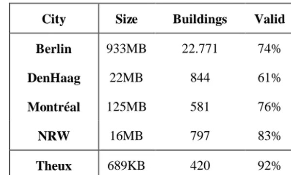
Table 1 provides a summary of the quality assessment for the open city models for international cities. Last line is the result of our method on the dataset provided by the Walloon Public Service. The area of interest concern the city of Theux, the chief town of a district in the south part of Belgium. The area counts residential buildings but also shops, sports hall, restaurant, etc. It is five hundred square meter wide and counts four hundred sixty four buildings. Note that the planarity tolerance for the other dataset has been set to 0.1 meters. Moreover, the planarity conformity is determined on a different basis in the SIG3D quality assessments. The least squares are preferred in this context.
City Size Buildings Valid Berlin 933MB 22.771 74%
DenHaag 22MB 844 61%
Montréal 125MB 581 76%
NRW 16MB 797 83%
Theux 689KB 420 92%
Table 1. Comparison to open models (from Ledoux, 2018) Only four hundred twenty buildings have been generated from the initial dataset. This is explained by the fact that not every building is considered as a building in regard of CityGML specifications (a building area should at least be greater than six square meters). Some garden sheds for instance are therefore filtered. Regarding the size, the difference comes from the fact that the other datasets are formatted in CityGML while our model is in CityJSON (see section 3 on 3D city models for explanation). No more information were given about the creation process of the other datasets. Finally, the methodology provides a very good quality for the geometries. First results show that the geometric validation reaches a level of 92% of consistent LoD 2.x buildings while the validation of the other datasets stabilized under 80%. However, even if these results are very promising, it appears that the segmentation methodology is the weak link during the process. Table 2 provides the detail of the quality control.
The International Archives of the Photogrammetry, Remote Sensing and Spatial Information Sciences, Volume XLIII-B2-2020, 2020 XXIV ISPRS Congress (2020 edition)
Error
Code Corresponding definition
Number of errors
101 Too few points 3
203 Non-planar plane 33
302 Shell not closed 3
303 Non manifold case 12
307 Polygon wrong orientation 8 Table 2. Overview of the validation results
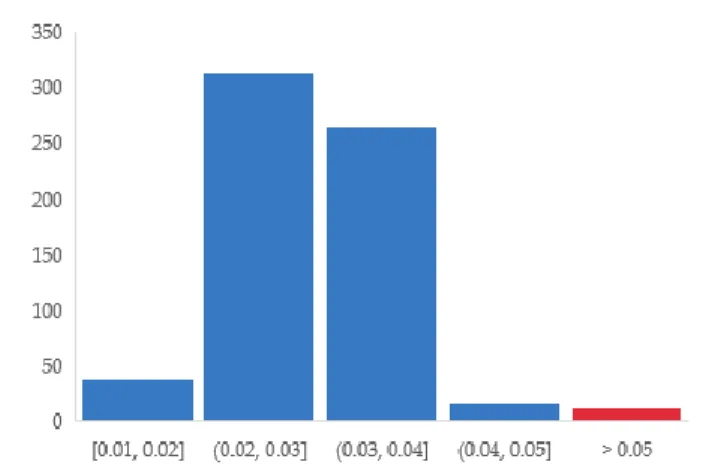
Even if the number of errors looks important in regard of the number of objects, these errors are spread over thirty-five buildings. Moreover, non-planar planes are limited to a much-reduced number of objects. The explanation of this concentration is due to the mean interpolation of the vertices height. As stated before, the error is spread on several planes within the same objects. This has the effect of multiplying their number but minimizing their relative impact. To estimate this non-planarity failure, the Root Mean Square Error (RMSE) has been computed on each detected plane, no matter the building to which they belong. Figure 4 classifies the RMSE into five classes of centimetric accuracy.
Figure 4. Planes per RMSE class
Six hundred forty four planes were tested. Among them, fifty-nine errors are counted. Point that sometimes, several errors occur on the same plane. Only eight planes have a RMSE greater than five centimetres. Those are actually extreme outliers as they greatly exceed one meter. Note that every point is considered in this calculus, not only inliers of every subset. Overall, the characteristics of the sample are good and little distributed:
Median: 0.028 meters 95th percentile: 0.039 meters
The quality control in a cascading way (from the object into its constituting parts) as proposed by the val3dity tool is a good point. Indeed, taking the example of a building where a single plane is missing, controlling every surface would not detect the hole: every vertex exist in other planes, topology between existing planes is correct, the majority of errors considered in Table 2 would not be encountered, semantic is coherent et the file format is verified also. The overall object must be evaluated to detect the inconsistency. It is explained by the fact
that many details for some cases cannot be reliably detected by the airborne LiDAR (windows, ventilation systems, etc.).
6. CONCLUSION AND FUTURE WORKS The automatic generation of compact city models from airborne LiDAR data still represents a challenge. Nonetheless, this paper provides an effective way to handle buildings generation concentrating compactness, expressivity and interoperability. Thanks to the promising CityJSON format, the generated model ensure topologic and geometric consistency. Compared to the current state of international cities, our results are promising. The simplicity and the effectiveness in regard of state of the art processes are also promising. However, to assess on its adaptability, the comparative analysis of the proposed methods should be performed on a set of common roof shape data such as RoofN3D. This dataset counts more than hundred thousand of buildings. This will bring information on the time consumption of the method and its scalability.
Since the geometric generation process already shows good results, future developments will study the semantic information support enrichment. The support of different classes of city objects (roads, bridges, vegetation) is a subject for future work. Such enhancement will open possibilities to cross-domain applications. Finally, the support of face-related information is a great improvement as materials and textures are important for visualisation purposes. Many applications in the Internet of Things or mobiles usages (autonomous cars, traffic management, etc.) would enjoy such compact city models.
REFERENCES
Biljecki, F., Ledoux, H., & Stoter, J. (2016). An improved LOD specification for 3D building models. Computers,
Environment and Urban Systems, 59, 25–37.
https://doi.org/10.1016/j.compenvurbsys.2016.04.005
Biljecki, F., Stoter, J., Ledoux, H., Zlatanova, S., & Çöltekin, A. (2015). Applications of 3D City Models: State of the Art Review. ISPRS International Journal of Geo-Information,
4(4), 2842–2889. https://doi.org/10.3390/ijgi4042842
Billen, R., Cutting-Decelle, A.-F., Marina, O., de Almeida, J.-P., M., C., Falquet, G., Leduc, T., Métral, C., Moreau, G., Perret, J., Rabin, G., San Jose, R., Yatskiv, I., & Zlatanova, S. (2014). 3D City Models and urban information: Current issues and perspectives: European COST Action TU0801. In R. Billen, A.-F. Cutting-Decelle, O. Marina, J.-P. de Almeida, C. M., G. Falquet, T. Leduc, C. Métral, G. Moreau, J. Perret, G. Rabin, R. San Jose, I. Yatskiv, & S. Zlatanova (Eds.), 3D City
Models and urban information: Current issues and perspectives – European COST Action TU0801 (pp. I–118).
EDP Sciences. https://doi.org/10.1051/TU0801/201400001 Gröger, G., & Plümer, L. (2012). CityGML – Interoperable semantic 3D city models. ISPRS Journal of Photogrammetry
and Remote Sensing, 71, 12–33.
https://doi.org/10.1016/j.isprsjprs.2012.04.004
Hu, P., Yang, B., Dong, Z., Yuan, P., Huang, R., Fan, H., & Sun, X. (2018). Towards Reconstructing 3D Buildings from The International Archives of the Photogrammetry, Remote Sensing and Spatial Information Sciences, Volume XLIII-B2-2020, 2020
ALS Data Based on Gestalt Laws. Remote Sensing, 10(7), 1127. https://doi.org/10.3390/rs10071127
Kurdi, F. T., Awrangjeb, M., & Liew, A. W.-C. (2019). Automated Building Footprint and 3D Building Model Generation from Lidar Point Cloud Data. 2019 Digital Image
Computing: Techniques and Applications (DICTA), 1–8.
https://doi.org/10.1109/DICTA47822.2019.8946008
Ledoux, H. (2018). val3dity: Validation of 3D GIS primitives according to the international standards. Open Geospatial
Data, Software and Standards, 3(1), 1.
https://doi.org/10.1186/s40965-018-0043-x
Ledoux, H., Ohori, K. A., Kumar, K., Dukai, B., Labetski, A., & Vitalis, S. (2019). CityJSON: A compact and easy-to-use encoding of the CityGML data model. ArXiv:1902.09155 [Cs]. http://arxiv.org/abs/1902.09155
Liu, X., Zhang, Y., Ling, X., Wan, Y., Liu, L., & Li, Q. (2019). TopoLAP: Topology Recovery for Building Reconstruction by Deducing the Relationships between Linear and Planar Primitives. Remote Sensing, 11(11), 1372. https://doi.org/10.3390/rs11111372
Poux, F., Neuville, R., Nys, G.-A., & Billen, R. (2018). 3D Point Cloud Semantic Modelling: Integrated Framework for Indoor Spaces and Furniture. Remote Sensing, 10(9), 1412. https://doi.org/10.3390/rs10091412
Schnabel, R., Wahl, R., & Klein, R. (2007). Efficient RANSAC for Point-Cloud Shape Detection. Computer
Graphics Forum, 26(2), 214–226.
https://doi.org/10.1111/j.1467-8659.2007.01016.x
Verma, V., Kumar, R., & Hsu, S. (2006). 3D Building Detection and Modeling from Aerial LIDAR Data. 2006 IEEE
Computer Society Conference on Computer Vision and Pattern Recognition - Volume 2 (CVPR’06), 2, 2213–2220.
https://doi.org/10.1109/CVPR.2006.12
Wang, R., Peethambaran, J., & Chen, D. (2018). LiDAR Point Clouds to 3D Urban Models: A Review. IEEE Journal of
Selected Topics in Applied Earth Observations and Remote
Sensing, 11(2), 606–627.
https://doi.org/10.1109/JSTARS.2017.2781132
Wichmann, A. (2018). Grammar-guided reconstruction of
semantic 3D building models from airborne LiDAR data using
half-space modeling.
https://doi.org/10.14279/DEPOSITONCE-6803
Xiong, B., Jancosek, M., Oude Elberink, S., & Vosselman, G. (2015). Flexible building primitives for 3D building modeling.
ISPRS Journal of Photogrammetry and Remote Sensing, 101,
275–290. https://doi.org/10.1016/j.isprsjprs.2015.01.002 Zhao, Z., Ledoux, H., & Stoter, J. (2013). AUTOMATIC REPAIR OF CITYGML LOD2 BUILDINGS USING SHRINK-WRAPPING. ISPRS Annals of Photogrammetry, Remote
Sensing and Spatial Information Sciences, II-2/W1, 309–317.
https://doi.org/10.5194/isprsannals-II-2-W1-309-2013
The International Archives of the Photogrammetry, Remote Sensing and Spatial Information Sciences, Volume XLIII-B2-2020, 2020 XXIV ISPRS Congress (2020 edition)