Forecasting for dynamic line rating

HAL Id: hal-01199238

https://hal-mines-paristech.archives-ouvertes.fr/hal-01199238

HAL is a multi-disciplinary open access

archive for the deposit and dissemination of sci-entific research documents, whether they are pub-lished or not. The documents may come from teaching and research institutions in France or abroad, or from public or private research centers.

L’archive ouverte pluridisciplinaire HAL, est destinée au dépôt et à la diffusion de documents scientifiques de niveau recherche, publiés ou non, émanant des établissements d’enseignement et de recherche français ou étrangers, des laboratoires publics ou privés.

Forecasting for dynamic line rating

Andrea Michiorri, Huu-Minh Nguyen, Stefano Alessandrini, John Bjørnar

Bremnes, Silke Dierer, Enrico Ferrero, Bjørn-Egil Nygaard, Pierre Pinson,

Nikolaos Thomaidis, Sanna Uski

To cite this version:

Andrea Michiorri, Huu-Minh Nguyen, Stefano Alessandrini, John Bjørnar Bremnes, Silke Dierer, et al.. Forecasting for dynamic line rating. Renewable and Sustainable Energy Reviews, Elsevier, 2015, 52, pp.1713-1730. �10.1016/j.rser.2015.07.134�. �hal-01199238�

1

Copyright notice: this is the self-archived version of an article proposed for publication in the journal

“Renewable and Sustainable Energy Reviews”; the copyright ownership of this document may change in the next future.

F

ORECASTING FOR

D

YNAMIC

L

INE

R

ATING

Authors

Andrea Michiorri, MINES ParisTech, France Huu-Minh Nguyen, University of Liege, Belgium Stefano Alessandrini, RSE, Italy

John Bjørnar Bremnes, Norwegian Meteorological Institute, Norway Silke Dierer, Meteotest, Switzerland

Enrico Ferrero, Universita del Piemonte Orientale, Italy

Bjørn-Egil Nygaard, Norwegian Meteorological Institute, Norway Pierre Pinson, Technical University of Denmark, Denmark Nikolaos Thomaidis, Aristotle University of Thessaloniki, Greece Sanna Uski, VTT, Finland

Corresponding author:

Andrea Michiorri, PhD

MINES ParisTech - Department of Energy and Processes

Centre PERSEE: Processes, Renewable Energies and Energy Systems 1, Rue Claude Daunesse - CS 10207 - 06904 Sophia-Antipolis, France Tel: +33 (0)4 93678977

2

ABSTRACT

This paper presents an overview of the state of the art on the research on Dynamic Line Rating forecasting. It is directed at researchers and decision-makers in the renewable energy and smart grids domain, and in particular at members of both the power system and meteorological community. Its aim is to explain the details of one aspect of the complex interconnection between the environment and power systems.

The ampacity of a conductor is defined as the maximum constant current which will meet the design, security and safety criteria of a particular line on which the conductor is used. Dynamic Line Rating (DLR) is a technology used to dynamically increase the ampacity of electric overhead transmission lines. It is based on the observation that the ampacity of an overhead line is determined by its ability to dissipate into the environment the heat produced by Joule effect. This in turn is dependent on environmental conditions such as the value of ambient temperature, solar radiation, and wind speed and direction.

Currently, conservative static seasonal estimations of meteorological values are used to determine ampacity. In a DLR framework, the ampacity is estimated in real time or quasi-real time using sensors on the line that measure conductor temperature, tension, sag or environmental parameters such as wind speed and air temperature. Because of the conservative assumptions used to calculate static seasonal ampacity limits and the variability of weather parameters, DLRs are considerably higher than static seasonal ratings. The latent transmission capacity made available by DLRs means the operation time of equipment can be extended, especially in the current power system scenario, where power injections from Intermittent Renewable Sources (IRS) put stress on the existing infrastructure. DLR can represent a solution for accommodating higher renewable production whilst minimizing or postponing network reinforcements. On the other hand, the variability of DLR with respect to static seasonal ratings makes it particularly difficult to exploit, which explains the slow take-up rate of this technology. In order to facilitate the integration of DLR into power system operations, research has been launched into DLR forecasting, following a similar avenue to IRS production forecasting, i.e. based on a mix of statistical methods and meteorological forecasts. The development of reliable DLR forecasts will no doubt be seen as a necessary step for integrating DLR into power system management and reaping the expected benefits.

3

KEYWORDS

4

ABBREVIATIONS

Above Ground Level (AGL)

Active Network management (ANM) Canadian Meteorological Centre (CMC) Computational Fluid Dynamic (CFD)

Consortium for Small-scale Modelling (COSMO) Direct Model Output (DMO)

Distribution System Operators (DSO) Dynamic Line Ratings (DLRs)

Electric Power Research Institute (EPRI)

European Network of Transmission System Operators for Electricity (ENTSO-E) Ensemble Prediction System (EPS)

Eulerian Autocorrelation Functions (EAFs)

Flexible Alternated Current Transmission Systems (FACTS) Grand Limited Area Ensemble Prediction System (GLAMEPS) High Resolution Limited Area Modelling (HIRLAM)

Information and Communication Technology (ICT) Institute of Electrical and Electronics Engineers (IEEE) Intermittent Renewable Sources (IRS)

International Council for Large Electric Systems (CIGRE) Limited Area Model (LAM)

Low Wind Speed (LWS)

Micro Electro Mechanical Systems (MEMS)

National Centre for Environmental Prediction (NCEP) National Oceanic and Atmospheric Administration (NOAA) Net Transfer Capacity (NTC)

Numerical Weather Prediction (NWP) Probability Density Function (PDF) Real Time Thermal Rating (RTTR) Red Electrica de España (REE) Return on Investment (ROI) Root Mean Square Error (RMSE) Transmission System Operator (TSO)

Weather Intelligence for Renewable Energies (WIRE) Wind Atlas Analysis and Application Program (WAsP)

5

1 INTRODUCTION

Dynamic Line rating (DLR, also referred to as dynamic thermal rating or real time thermal rating) is a technology that can dynamically increase the current carrying capacity of electric transmission lines. It is based on the observation that the ampacity of an overhead line is determined by its ability to dissipate into the environment the heat produced by Joule effect. The ampacity of a conductor is defined as the maximum constant current which will meet the design, security and safety criteria of a particular line on which the conductor is used [1]. This in turn is dependent on environmental conditions such as the value of ambient temperature, solar radiation, and wind speed and direction. Currently, only conservative seasonal estimations of meteorological values are used to determine ampacity. In a DLR framework, ampacity is considered as a dynamic variable giving a conservative estimate of the critical value at which the line may be operated at each time unit of operation. This phenomenon is particularly obvious on overhead transmission lines, where DLR can provide considerable uprating. In the current power system scenario, where the rise of power from Intermittent Renewable Sources (IRS) puts stress on the existing infrastructure, making network reinforcements necessary, DLR can represent a solution for accommodating higher renewable production whilst minimizing or postponing network reinforcements. Furthermore, similarly to IRS production forecasts, the development of reliable DLR forecasts is seen as a necessary step for integrating DLR into power system management and reaping the expected benefits. Practices in power system operations are expected to evolve dramatically in the coming years under the pressure of an increasing share of renewable and intermittent energy generation in the energy mix and a changing environment due to the liberalization of electricity markets. The consumption patterns of end-consumers are also evolving, and more interactions are expected in the future, e.g. in the case of demand-side management. An overview of the challenges of wind power generation is given in [2] while some of the key issues and potential benefits of more proactive participation of electric demand in power system operations (potentially through electricity markets) can be found in [3]. It is worth mentioning that the share of solar energy in the electricity mix is sharply increasing and will represent a substantial proportion of the electricity mix in the future.

Transmission and distribution networks are conservatively dimensioned, resulting in a typical usage rate lower than their maximum transmission capacity for security reasons. This is because the system is planned and operated in order to guarantee the highest possible security and quality of supply, which involves using conservative worst-case assumptions at the planning stage. Furthermore, recent work [4] illustrates how wind power generation, or similarly, electricity prices, could highly influence power flows over the whole European power system governed by the European Network of Transmission System Operators for Electricity (ENTSO-E) and operated by its member TSOs. Such a situation calls for reinforcing and further developing the network from a strategic point of view, and accounting for the characteristics of such power flows as influenced by renewables, with their generation patterns of strong spatial correlations [5]. The evolving context of electricity markets also needs to be considered as part of the transmission expansion problem [6].

Transmission expansion planning is associated with longer time scales, since new lines typically take 5 to 10 years from the initial planning stage to construction and operation, and require massive investment (up to hundreds of thousands of euro per km) and social acceptance. Meanwhile, innovative solutions are being sought in a smart grid context, with increased capabilities for monitoring and communicating

6

relevant information, combined with solid modelling and control approaches. Among the approaches studied over recent years, DLR has the potential to unlock latent network transmission capacity, delay network reinforcements, and facilitate the connection of renewables to the grid. Arguably, integrating DLR into power system operations may result in higher penetration of renewable energy, reduced greenhouse gas emissions [7] and increased social welfare in coupled electricity markets by lowering overall generation costs.

In order to incorporate DLR in TSOs’ operational practices, reliable ampacity forecasts need to be available for specific lines or the full network. This challenge has already been highlighted in the relevant literature, such as the pioneering works by Hall and Deb [8], Douglass [9] and Foss [10]. In today’s context, the time scales involved are in line with electricity markets where most operational decisions are made the day before operation: DLR forecasts should employ lead times roughly between 12 and 36 or 54 hours. Forecasts should also be available with a resolution specified by the users’ needs (from minutes to hours).

This document is structured as follows: a historical perspective on the DLR challenge and the renewed interest in this concept are first presented in Section 2. Section 3 provides a review of some of the key characteristics of the DLR forecasting problem, covering the known relationship between meteorological variables and corresponding line rating, and the issue of predicting these meteorological variables is reported in Section 4. Finally Section 5 introduces the mathematical framework for forecasting and verification, applications and foreseen benefits are presented and discussed in Section 6, before the concluding remarks in Section 7.

7

2 HISTORICAL AND PRACTICAL PERSPECTIVES

Research related to DLR is based on investigations on overhead conductor ratings, which started before World War 2. In 1958, House and Tuttle at Alcoa Research Laboratories (USA) suggested the steady state ampacity model [11]) which is basically the one currently used. About ten years later, Morgan [12] at the National Standards Laboratory of Sydney (AU) proposed a similar steady-state rating model, while [13] and [14] at Jersey Central Power (USA) proposed dynamic models for describing the thermal behaviour of conductors. These models are the basis of the International Council for Large Electric Systems CIGRE [1] and Institute of Electrical and Electronics Engineers (IEEE) [15] models still broadly used today. These standards will be referred to simply as the CIGRE standard or IEEE standard throughout the document. The possibility of using variable line ratings to increase line utilization was studied for the first time by Davis at the Detroit Edison Company (USA) who, between 1977 and 1980 published a series of texts [16][17][18][19][20] on different aspects of the problem, calculating daily and hourly ratings and comparing the actual rating distribution with the rating-risk curve applied.

Research continued with the group of Foss, Lin and Maraio at General Electric (USA) [21][22][23][10] who in the years 1983 – 1992 further developed the models and studied their dependence on each variable. [23] also reports the results of one of the first monitoring campaigns of the temperature of different points on an overhead line, and proposes the first method for DLR forecasting based on weather forecasts. During the same period, the first patent [24] for an overhead line temperature monitoring system was granted to Fernandes and Smith-Vaniz of the Niagara Mohawk Power Corporation.

Another research group was active around Douglass and Edris at Power Technologies and the Electric Power Research Institute EPRI in the USA [25][9][26][27][28]. From 1988 – 2000 they integrated a software for calculating dynamic thermal ratings for several power system components (not only overhead lines) in substation controls and tested it at four utilities in the USA. The system they developed employed thermal measurements and interpolated ratings using semi-empirical parameters. Another system, described by Seppa [29][30] at The Valley Group (USA), was based on measuring conductor tension and used cellular telecommunication to retrieve data from several locations. In 2000, according to [31] more than 50 utilities used a transmission line monitoring system on one of their lines to evaluate its thermal limitations, and most of these were based on a tension measurement method. The system described is also partially covered by a patent [32], and in 1999 a patent [33] was awarded to a weather-based ampacity calculation software.

Among the different methods proposed for estimating DLRs, it is also worth mentioning the use of differential GPS [34][35] at Arizona University, the use of phasor measurement [36][37] also covered by a patent [38], and the measurement of conductor vibrations [39] at the University of Liege in 2010, also covered by a patent [40]. Comprehensive DLR systems reviews and good operational practice recommendations are mentioned in technical brochures by international engineering organizations [1]. From an early stage, DLR technology was tested by several utilities and records of several pilot projects exist. In Europe, an early example is the DLR system developed by Red Electrica de España (REE) and Iberdrola in 1998 [41], where a minimal number of meteorological stations were used to gather real-time data. The data was then processed using a meteorological model based on the Wind Atlas Analysis and Application Program (WAsP), taking into account the effect of obstacles and ground roughness, and

8

finally the rating was calculated. Another test was carried out by Nuon in 2004 [42] and consisted of a fiber-optic-based temperature monitoring system for electric cables, power transformers and overhead lines. In recent years, the application of DLRs has been studied and tested, particularly in the UK, for accommodating new wind power generation by Central Networks (Yip, 2009), Scottish and Southern Energy [43], Iberdrola Scottish Power [44][45][46] and Northern Ireland Electricity [47], and also the Belgian ELIA [48]. The situation is different for solar radiation, as few dedicated applications exist. Note that the characteristics of solar radiation (frequency distribution) are different from wind power.

The study of DLRs has proceeded almost continuously for more than thirty years, mainly in the USA, and by different groups. The predominance of American research may be explained by the fact that the USA experienced summer peaks before European countries, leading to more research and development on the physical limits of conductors. Several techniques have been developed around the world for real-time DLR, such as measuring conductor temperature, tension and vibration, but for long-term forecasts the greatest potential is clearly the estimation of DLRs from weather parameters combined with in-situ measurements. Recently, focus on this technology has increased because of the development of Micro-Electro-Mechanical Systems (MEMS), IT, and wireless communications, and its potential consequences on the integration of IRS, and the subsequent appearance of network congestions, particularly in Europe but also in the USA and Asia.

9

3 THE IMPACT OF WEATHER PARAMETERS ON LINE RATINGS

Overhead line ratings are constrained by the necessity to maintain statutory clearances between the conductor and other objects or the ground. DLR is based on the concept that overhead line rating is limited by a maximum conductor temperature in order to respect these clearances and preserve mechanical integrity. Although the conductor’s temperature is dependent on the electrical load, it is also strongly influenced by environmental conditions, such as wind speed, air temperature, and incident radiation.. But variable conductor temperatures on the line can modify the span sag by up to several metres, depending on the mechanical tension and the length of the span. In fact, a rise in temperature causes the conductor to elongate which, in turn, increases the sagging. A schematic vision of an overhead line and its sag and clearance is provided in Figure 1.

Figure 1: Sketch of Sag (S) and Clearance (C) of an overhead conductor in a level span. (courtesy: Ampacimon)

The sag S [m] can be modelled as a catenary equation or as its parabolic approximation, given by:

(1)

depending on conductor properties (mass per unit length m [kg·m-1], span length L [m]) and the horizontal component of the conductor tensile force (H [kg.m.s-2]), which depends in turn on the thermal-tensional equilibrium of the conductor [49].

– – . (2)

In the above formula,

- A [kg.m.s-2K-1] and B [kg3.m3.s-6] are parameters depending on conductor properties such as the thermal elongation coefficient, Young’s modulus, and the cross sectional area, conductor mass, and span length,

- Tc [K] is the conductor temperature,

- H is the horizontal component of the tension and the subscripts 1 and 2 refer to two different

10

A reference state 1 can be relative to standard design conditions, whilst state 2 changes according to temperature. Therefore a one-to-one relationship can be modelled between the span sag (and hence the clearance) and the conductor’s mean temperature over that span, and more generally over the line section [50] [51].

However, it should be pointed out that standard design conditions are seldom respected in practice (e.g. plastic elongation due to initial tensioning and severe ice/wind loads, metallurgical creeping, installation conditions, etc.). Furthermore, it is difficult to measure the mean conductor temperature on which the sag (and thus the clearance) depends.

3.1 DYNAMIC THERMAL MODE L FOR OVERHEAD LINES

IEEE and CIGRE models have been regularly updated since they were first proposed and are frequently used by engineers as calculation standards to assess the thermal behaviour of overhead lines. Despite some differences in their detailed formulation, the approach followed is similar and the conductor steady-state temperature results from a heat balance:

(3)

where:

- Qs [W/m] is the solar heating depending on solar radiation and albedo,

- Qr [W/m] is the radiative cooling depending on conductor and ambient temperature (as a first

approximation),

- Qc [W/m] is the convective cooling, mainly influenced by wind speed and direction,

- I [A] is the conductor electrical load

- R(Tc) [/m] is the conductor’s electrical resistance per unit length at the specified conductor

temperature.

The main difference between the IEEE and CIGRE models lies in the expression of the convective term Qc, which is also the prevailing term for conductor cooling. This term is essentially driven by wind speed, with a dramatic impact at low wind speeds (<5m/s). These different formulations result in significantly different line ratings for low wind speed values. However, the two models yield similar results for the design wind speed (usually in the region of 0.5 m/s). Both the IEEE and CIGRE models now include a fairly comprehensive solar irradiance model that takes account of the geographic position, altitude and time of year.

The non-steady-state heat balance is the same 1st order differential equation for both models:

[ ] (4)

where:

- m [kg/m] is the mass per unit length of conductor material

11

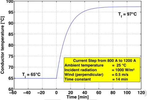
This results in a time constant of about 10-20 minutes for the design wind speed for most of the conductors. The time constant can decrease to only 5-10 minutes for higher wind speeds (> 3m/s). An illustration of the transient temperature response is given in Figure 2.

Figure 2: Transient temperature response to a “step” change in current. Three to four time constants are needed to reach the steady state; this dynamic aspect can be used by the TSO, as in a N-1 situation1, it takes about 1 hour for the conductor to reach the steady-state temperature at the design wind speed (about 0.5 m/s) [AMS570 conductor].

3.2 RELATIVE IMPORTANCE OF ENVIRONMENTAL P AR AMETERS

The influence of the four environmental parameters on the conductor rating is variable because of the non-linearity of the heat exchange mechanisms. This makes it impossible to reduce the study to a particular parameter and force a DLR system to take the value of all of the environmental parameters involved into account.

As reported in [45], wind speed is the most important variable for mid-range wind speed values, although the sensitivity of ampacity vs. wind speed is higher for low wind speed values. In parallel, the worst operating conditions for overhead lines occur in cases of low wind speed, when air temperature and solar radiation become critical factors. In an operational context, where all of these variables evolve rapidly and dynamically, the influence of all of these variables should be monitored and predicted. These variables include wind speed (Ws), wind direction (Wd), ambient temperature (Ta), and solar radiation (Sr).

1 _{The N-1 principle guarantees that the loss of any set of network elements is compatible with the system’s} operational criteria, taking into account the available remedial actions. For power lines, in practice this means keeping some line capacity reserve for each line in operation. It ensures that if one line trips, the additional electrical load shifted onto other lines will not lead to cascade tripping.

12

The relative impacts of weather variables are further described and discussed in the following paragraphs and in [52]. They are analyzed based on observations of the variables involved, and on IEEE and CIGRE standard models for overhead line rating. The nature and strength of such relationships between meteorological variables and overhead line rating should be appraised in a different manner when considering a forecasting setup perspective.

The case of solar radiation is particularly interesting: its effect is in general negligible since other parameters, notably wind speed, have a far larger impact on the cooling of the conductor. However, in low wind speed conditions, it can considerably increase the temperature of the conductor, also with low current values, and thus become a significant limiting factor.

Line icing and its impact on ratings forms a specific topic that includes studying effects such as over-sagging due to ice load, non-uniform icing, modification of the state-change equation, galloping and other vibration issues, etc. Thus, icing will not be discussed in this document.

Another aspect to be considered is the sensitivity of measurement equipment, which can vary according to the parameter measured and its impact. For example, air temperature can be measured accurately with respect to determining ampacity during the calculation process, whilst effective wind speed along the whole line section cannot (in particular for low wind speeds).

It should also be considered that environmental parameters, and in particular wind speed and direction, may change considerably along the path of a transmission overhead line. Indeed, the exploitable ampacity actually unlocked by DLR corresponds at any time to the minimum of all ampacities calculated for each critical span in the line. Therefore, a DLR system and a DLR forecast must take into account this phenomenon and provide estimates of the actual current carrying capacity for the whole line.

3.2.1 WIND SPEED

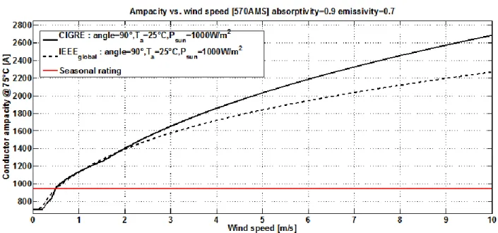
Wind speed has a prevailing impact on power line ampacity as it is the main variable responsible for cooling down the conductor, and hence for the sag value. Its influence is illustrated in Figure 3, based on the CIGRE and IEEE standards and for a given set of standard conditions with respect to wind angle relative to the conductor, temperature and incident radiation.

13

Figure 3: Relationship between wind speed and conductor ampacity, following the CIGRE/IEEE standards, for a set of other environmental variables for an AMS570 conductor rated at 75°C. The differences between the two standard models decrease near the seasonal rating due to the fact that the empirical equations used to calculate convective heat exchange are centred on the conservative conditions of very low wind speeds.

Although the relationship between wind speed and ampacity is clearly defined in the IEEE and CIGRE standard models, in practice such dependence may be more complicated to establish and observe, since wind speed varies in time along the length of each span and vertically.

First, wind speed exhibits significant temporal variability in magnitude and even in the nature of its dynamics, evolving significantly within minutes [53] and hence challenging the steady-state representation of the various standard models. Second, the spatial variability in wind is such that wind speed also varies along the span (spatial coherence), wind vortices having a typical average size of several tens of metres [54]. Therefore, a typical span length of several hundred metres is subject to a variable wind speed along its length. Third, wind speed also varies greatly vertically, as the conductor is located within the boundary layer. Wind speed may also vary due to local effects, such as screening from trees or buildings. Note that the elevation of the conductor may change by more than 15 metres in a single span. Consequently, the sag may also be subject to differences in level between the end points of a span. Such elevation differences near the ground may have huge effects on the wind characteristics, which are highly sensitive to changes in elevation so close to the ground.

On a line section made up of multiple spans linked to each other via suspension insulators, the horizontal component of the tension – and thus sag - is balanced to a certain extent [55]: therefore, the behaviour of a single span (typically 400 m length) within a line section depends on all the other spans in the same section. This means that environmental parameters, such as wind speed or wind direction varying over several tens of metres, should normally be considered for the whole section. The integrated effect of high frequency wind variations can also be used to calculate the mean effect of wind on ampacity since the dynamic behaviour of the conductor (time constant) acts as a filter.

14

3.2.2 WIND DIRECTION (AND ITS ANGLE WITH LINES)

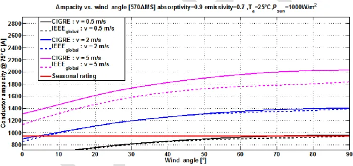
Wind angle is defined as the angle between the wind vector and the conductor axis of the span of interest. Figure 4 shows the relationship between wind angle and ampacity, based on IEEE and CIGRE standards, and for various sets of wind speed, incident radiation and ambient temperature. In addition to wind speed, wind angle may have a non-negligible impact on ampacity, especially for almost-parallel wind flows. In practice, due to turbulence, the variation in conductor temperature and line ratings caused by wind direction is substantially lower than assumed based on theoretical DLR calculations. Therefore conservative assumptions are usually made. For example, on hot summer days with low wind speeds, the standard deviation of the wind angle is typically about 45 degrees or more [56]. In such situations, the effective yaw angle of the wind is set between 35 and 45 degrees (depending on user practices) irrespective of the average wind direction [57].

For this reason, the concept of “effective” wind speed has been introduced: effective wind speed is defined as the equivalent perpendicular wind speed that produces the same cooling effect as the actual wind. The wind angle is considered only under laminar conditions, e.g. with a standard maximum deviation of 20 degrees, which can occur at night.

Figure 4: Relationship between wind angle (i.e., angle between wind vector and the span direction) and conductor ampacity, based on IEEE/CIGRE standards, and for various sets of other environmental variables for an AMS570 conductor rated at 75°C, Ta=25°C, Psun=1000W/m2).

3.2.3 AMBIENT TEMPERATURE

Ambient air temperature has a significant impact on ampacity, as illustrated in Figure 5. This effect is quasi linear considering a limited range of temperatures and substantial for all temperature levels in a temperate climate range. A Root Mean Square Error (RMSE) < 2°C in the modelling or forecasting of ambient temperature may be considered satisfactory. This is easily achievable using weather stations and

15

state-of-the-art meteorological forecasting approaches. Another advantage is that the temperature varies little over the time and spatial scales of interest here, except perhaps in highly complex areas, for instance from one valley to the next in mountainous terrains.

It should be also considered that ambient temperature influences both convective and radiative heat exchange, with an almost linear effect on ampacity behaviour shown in Figure 5.

Figure 5: Relationship between ambient temperature and conductor ampacity, based on IEEE/CIGRE standards, and for various sets of other environmental variables for an AMS570 conductor rated at 75°C, angle=90°, Psun=1000W/m2).

3.2.4 PRECIPITATION

Rain has a significant impact on conductor cooling but, as heat loss rate modelling requires several parameters, such as the water’s physical state, relative humidity, precipitation rate, wind speed, and air pressure, it is often neglected in line design standards. However, for DLR, as the ampacity is computed dynamically, rain cannot be put aside completely. Precipitation information gathered from observations or forecasts can be valuable for computing a conservative ampacity using a somewhat simplified model. An example of an overhead conductor rating model incorporating the role of precipitation can be found in [58][59].

3.2.5 SOLAR RADIATION

Similarly to wind speed, a single-point measurement of effective incident radiation is not sufficient to compute the global combined effect of solar irradiance and albedo over a whole span. Its influence can be considered linear for this application. This is represented in Figure 6 based on the IEEE and CIGRE standards, for various sets of other environmental variables. For very low wind speed conditions (Ws<0.5 m/s), solar radiation can become a limiting factor for overhead line ampacity, since it can raise the temperature of the conductor far above the air temperature.

16

Figure 6: Relationship between incident radiation and conductor ampacity, based on IEEE/CIGRE standards, and for various sets of other environmental variables for an AMS570 conductor rated at 75°C, angle=90°, Ta=25°C).

0 100 200 300 400 500 600 700 800 900 1000 800 1000 1200 1400 1600 1800 2000 2200 2400 2600 2800 Incident radiation [W/m2] C o n d u c to r a m p a c it y @ 7 5 °C [ A ]

Ampacity vs. Incident radiation [570AMS] absorptivity=0.9 emissivity=0.7 ,angle=90°,T

a=25°C CIGRE : v = 0.5 m/s IEEE global : v = 0.5 m/s CIGRE : v = 2 m/s IEEE global : v = 2 m/s CIGRE : v = 5 m/s IEEE global : v = 5 m/s Seasonal rating

17

4 METEOROLOGICAL MODELLING AND FORECASTING CONSIDERATIONS

4.1 METEOROLOGICAL AND FORECASTING MODELS RELEVANT TO DLR

The basis for meteorological modelling and modern weather forecasting was laid down in the early 20th century, when it was established that if the state of the atmosphere is known at any point in time, its future state can be determined using the fundamental laws of standard physics. The standard principles in fluid mechanics of mass conservation, and momentum change due to mechanical forces, were combined with the standard fundamental laws of thermodynamics to produce a closed set of non-linear, partial differential equations (thermo-hydrodynamic equations). These equations give time tendencies of the standard meteorological variables, wind, pressure, temperature, and humidity, in any part of the atmosphere, provided their values are given in the entire atmosphere at a given time (the initial state, also called the analysis) and at any time at the top and bottom of the atmosphere (the boundary conditions). Fundamental mathematical theory predicts that a single solution to the equations with the given initial and boundary conditions exists. As such, the problem of weather prediction is formally deterministic. However, practical solution methods for general cases are not known. Thus, systematic simplifications and discretization of the equations in time and space are necessary to find an approximate solution. The outcomes of this process are numerical models of the atmosphere, which for the purpose of weather forecasting, are referred to as Numerical Weather Prediction (NWP) models. The numerical discretizations and other approximations necessitate so-called parameterizations, which are empirical formulae that represent the effects of the simplifications. NWP models are computationally very demanding and some of the most powerful supercomputers are today employed for this purpose [60].

The horizontal domain of a NWP model is either global, covering the entire earth, or regional, limited to a smaller area. Due to atmospheric motions, a global domain is required for forecast horizons beyond three or four days. For shorter horizons, computational resources often focus on a smaller domain implying the possibility of higher spatial resolutions and more accurate modelling of the physical processes. The latter so-called Limited Area Models (LAMs) are, however, dependent on forecasts from global models at the boundaries of their domains. Most of the systems being developed are NWP systems, run on an operational basis by national meteorological services and universities. To date, there are roughly ten operational NWP models for the global domain, running with horizontal resolutions between 15 and 40 km. For smaller domains, typically a few thousand kilometres in each direction, LAMs run with a horizontal resolution of a few kilometres. For special applications, NWP models with even finer horizontal resolutions are also applied.

Weather forecasts are calculated using LAMs that simulate atmospheric flows from synoptic scale to a few kilometres. These solve the averaged Navier-Stockes equation and parameterize turbulence using different schemes, which entail diffusion coefficients and turbulent kinetic energy. The equations are solved on different nested grids. The resolution of the inner grid is usually two kilometres, while the ratio between the resolutions of the different grids is about four. Topography is usually introduced using terrain-following vertical coordinates. Schemes are determined for the lateral boundary conditions and the radiation parameters for evaluating both shortwave radiative transfer and long wave radiation.

The process of making weather forecasts starts by collecting measurement data from satellites, radars, aircrafts, ships, buoys, radiosondes and conventional instruments at the Earth’s surface for a relatively large geographical area. To achieve this, all countries share a huge amount of observational data using fast

18

telecommunication networks. Information from the measurements is then extracted in a dynamic and consistent way to estimate the state of the atmosphere on a three-dimensional spatial grid at a given point in time. The irregularly spaced observations are insufficient on their own. The best estimates are obtained by combining these observations with a previous forecast in a process known as data assimilation. Data assimilation provides initial conditions for forecast models, which then are integrated forward in time, step by step with time resolutions in the order of seconds/minutes until the required length of forecast has been reached. Forecast models are very complex due to a large number of mathematical and physical challenges that must be considered - ranging from numerical aspects in the dynamical part of the model to parameterizations of physical processes that are too small in scale or too complex to be modelled explicitly.

National Meteorological Services (NMS) are required to provide short- and medium-range weather forecasts, warnings and alerts for their territory. Medium-range forecasts require global models such as those provided by the European Centre for Middle Range Weather Forecast (ECMWF) or the National Oceanic and Atmospheric Administration (NOAA). For short-range applications, it is more cost effective, and even necessary for very high resolution, to run the Numerical Weather Prediction (NWP) systems for only a limited part of the globe using an LAM. These LAMs require boundary conditions from global models, like the ECMWF model.

4.2 INCREASING ROLE OF METEOROLOGICAL FORECA STING IN POWER SYSTEMS OPERATIONS

With the further deployment of renewable energy generation capacities in Europe, but also in the US, China, etc., it is clear that power generation is increasingly reliant on the weather and climate. Power generation from most renewable energy sources is a direct function of the onsite meteorological conditions. This is the case for wind farms and solar panels, which are at the origin of the increasing role of meteorological forecasting in power system operations, especially over the last few decades. Hydro power is also directly dependent on weather conditions, but its different time dynamic makes it much less variable than the previously mentioned renewable sources. A comprehensive, recent overview of the importance of weather and climate for energy-related problems is given in [61].

Prior to the recent large deployment of renewable energy capacity, a number of researchers and practitioners had already observed that the electrification of heating and cooling in a number of areas of the world was making electricity consumption increasingly sensitive to ambient temperature. Consequently, temperature forecasts became the first and most relevant type of meteorological information to take part in power system operations, following the pioneering work of Papalexopoulos and Hesterberg [62] among others. Note that in addition, the relatively high accuracy of temperature forecasts make them an ideal input for load forecast algorithms. Meteorological information for renewable energy forecasting, and dynamic line rating forecasting prediction in particular, is more complex. The methods used for electric load forecasting have thus been gradually extended to a probabilistic framework, for instance based on overall temperature forecasts, discussed below. As an example, the reader is referred to [63].

19

In comparison, since the beginning of the new millennium, renewable energy generation (first wind power, then solar power) has been the main driver for using basic and advanced meteorological forecasting products in power system operations. The focus has also shifted to variables that were formerly considered less important. For instance, the accuracy of wind predictions had been considered sufficient for most applications, but with the sensitivity of wind turbines’ power output to changes in wind speed/direction, even small errors in wind forecasts can lead to significant errors in power predictions. Similarly, the need for additional variables has become apparent, for instance related to solar radiation or to a better description of wind profiles. Recent overviews and discussions of load and renewable energy forecasting can be found in [64] and [65]. The renewed interest in the impact of the weather on electric lines will also potentially strengthen the focus on various types of meteorological predictions.

4.3 DOWNSCALING

Wind speed depends both on atmospheric conditions and topographical features. Different stability conditions develop during the daily cycle, and particularly during the night, when the stable boundary layer creates conditions for low wind speeds. Wind velocity is influenced by surface roughness, topography features such as the presence of flat or complex terrains, and the presence of a coastline. Mountains act as shield for the wind, which descends low into valleys, and breeze circulation may develop.

Wind speed and direction have a high temporal and spatial variability. Significant changes in wind speed and direction in the space of a few metres are caused by obstacles, terrain and roughness changes in the vicinity of the span. In order to consider these effects in a weather forecast model, meter-sized grid sizes would be required. However, the grid sizes on today’s high-resolution weather forecast models are in the range of about 1 km. Thus, important impact factors are not resolved in the models. Regarding ampacity, though, the effect of weather parameters is integrated over the span’s length, and more generally over each line section, leading to less constraining requirements on the grid size.

Different methodologies exist to refine the results of weather forecast models. These methods basically fall into two groups: statistical and dynamical downscaling procedures.

Statistical downscaling describes the relationship between the results of weather forecast models and measurements using statistics, e.g. multiple linear regressions or Kalman filtering. These methods are well tested for wind forecasting for wind power predictions and result in significant improvements compared to Direct Model Output (DMO) from weather forecast models. Statistical methods require on-site measurements/estimations of wind speed and direction. However, measurements are not available at every point of interest and additional methods are needed for e.g. spatial interpolation. An example is a method that interpolates in space the coefficients of a multiple linear regression in order to obtain forecasts for positions between the measurement sites [66]. This and other similar methods need to be tested in the framework of DLR, especially in complex terrains.

An alternative approach is dynamical downscaling. Dynamical downscaling increases the spatial resolution of weather forecast models by applying higher resolution dynamical models. This kind of grid size requires switching to LES or Computational Fluid Dynamic (CFD) models.

20

A common method for simulating a wind field is the mass-consistent model. This is a diagnostic model based on mass conservation for incompressible fluids (∇·u=0). Measurements are interpolated on a high-resolution (up to 100 m) grid. Stationary conditions are assumed and the turbulence is not simulated. More sophisticated models account for turbulence. Three main approaches can be considered.

- Reynolds-Average models (RANS) - Direct Numerical Simulation (DNS) - Large Eddy Simulation (LES)

In a RANS model, mesoscale models resolve the equation for the mean values of each parameter but parameterize the turbulence in an approximated way. In a DNS approach, the equations for the second order moments (Reynolds stress) are solved and a closure problem arises. To prescribe these quantities, on which the mean values depend, dynamical equations must be resolved. These equations entail the third-order moments, which in turn depend on the fourth-third-order moments and vice versa. Therefore a closure hypothesis is needed. Generally the fourth-order moments are expressed as a function of the second ones, assuming a Gaussian probability density function of at least this order, [67][68][69]. Unfortunately this approximation does not apply in low-wind conditions [70]. In this model, Navier-Stokes equations are resolved at all scales. This implies a very high computational power and as a consequence Reynolds numbers, as those of the atmosphere cannot be reproduced. However, DNSs are useful for theoretical studies.

In an LES approach, turbulence is divided into so-called “large eddies” containing most of the energy, which are directly resolved, and so-called “sub-filter scale eddies” with low energy content, which are not resolved but parameterized. LES is generally used to simulate the stationary atmospheric boundary layer in different stability conditions but it can be also nested in the mesoscale models. The sub-filter-scale model makes the hypothesis that LES is not sensitive to the sub-scale filter itself, but the model is not totally reliable close to the surface, where smaller scale eddies develop.

Several studies have tested LES for wind energy applications. In simple terrains, the effect was found to be small [71], while other studies showed good results in complex terrains and for flow around obstacles [72]. LES involves large amounts of computing time, which explains why it is currently not possible to run online-forecasts. It could, however be used in a statistical-dynamical approach.

CFD models are often used for wind resource assessment to simulate the flow field in complex terrains. CFD models are run with grid sizes as small as a few metres and thus allow a fine resolution of obstacles and terrain features. Unfortunately, CFD models’ ability to correctly simulate situations with low wind speeds is not yet proven. Additionally, CFD models do not cover important atmospheric processes that might be relevant for local circulation systems, like radiation or clouds. This shortcoming is tackled by coupling CFD models with weather forecast models, whereby local flow regimes are simulated by the weather forecast model and the flow field is refined by the CFD model. First studies show promising results [73].

Dynamical-statistical downscaling is used to keep the forecasting computation time short: it describes an approach where relevant weather situations are defined, refined to very high resolution by dynamical downscaling, and correction factors are derived. The daily weather forecasts are classified according to the

21

relevant weather situations and the correction factors are applied. These methods have been successfully applied in the framework of regional climate modelling and also in wind power forecasting [74][73].

4.4 FOCUS ON LOW WIND SPEEDS

Low Wind Speed (LWS) conditions, roughly defined as periods when the mean wind speed at 10 m a.g.l is less than 2 m·s-1, are particularly important for the science of air pollution dispersion because it is under such conditions that the severity of pollution is often high due to weak dispersion [75]. Despite their considerable practical interest, LWS are difficult to predict, especially in conditions of strong atmospheric stability when the state of the lower atmosphere is not well defined.

Due to the non-linearity of a conductor’s thermal behaviour, wind speed and in particular LWS is considered as a critical parameter. Furthermore, low wind speeds are expected to be the limiting parameter in a DLR forecast application and an accurate forecast of this parameter is considered crucial for R&D. However, in operational practice, the important information is the probability of LWS occurrence, which is the information that TSOs require. As forecasting LWS will remain difficult in the near future, standard rating may continue to be used in such cases.

LWS is a very common condition in many European areas, for example, in the Po valley in Italy, which is characterized by frequent low wind speed conditions. More than 80% of mean wind measured there is u < 1.5ms−1 at 5m a.g.l, probably due to the shielding effect of the surrounding mountains and hill chains. The rare cases of strong wind are caused by the dry down-slope wind from the Alps, also known as “Foehn”, which occur in the cold season typically about 15 times per year.

4.4.1 LOW WIND CHARACTERISTICS

Most papers proposed in literature on low wind focus on the dispersion issue. The turbulence, e.g. the standard deviation of the wind velocity fluctuation, needs to be determined in order to provide input for a dispersion model.

LWS can have different origins, but in general it is associated with stable atmospheric conditions, such as high atmospheric pressure. LWS can also originate at night when the ground surface cools down and creates a stable temperature gradient in the surface layer.

Important aspects for the study of LWS are:

- Meandering

- Turbulence statistics

Meandering is defined as the slow oscillating motion of airflow. Oettl and Goulart [76][77] suggested that meandering is an inherent property of atmospheric flows in low-wind speed conditions and generally does not result from any particular trigger mechanism. According to those works, meandering can exist in all meteorological conditions, regardless of the atmospheric stability, specific topographical features, or season, provided the average wind speed is less than about 1.5 ms−1.

22

The causes of meandering vary. One possible cause is the vertical directional shear induced by a terrain. Gravity waves, vortices with either a horizontal or vertical axis, and so-called vortical modes, are potential mechanisms for generating a meandering flow. A stable stratification of the boundary layer is seen as a necessary pre-requisite for obtaining a meandering flow regardless of the possible processes initiating it. The meandering scale lies in between the turbulence scale and the mesoscale. A parameter sometimes used to detect meandering is the standard deviation of the crosswind component σv scaled by the friction velocity [78][79]:

(5)

where is the friction velocity, z the height above the ground and L the Monin-Obhukov length which indicates the stability. This quantity indicates the extent of the wind lateral fluctuations, which are determined by the turbulence and, in the LWS case, by the horizontal meandering as well.

Regarding turbulence statistics, LWS presents specific features in its auto-correlation function and Eularian auto-correlation function. The horizontal wind velocity autocorrelation functions do not fit in with an exponential decay but display oscillating behaviour [78] probably determined by horizontal coherent structures. Another characteristic is that the horizontal Eulerian Autocorrelation Functions (EAFs) are not exponential (as in a windy case) but rather reveal a negative lobe and an oscillating behaviour. Also, in low wind conditions, the higher order of the probability density function reveals specific behaviour. In normal conditions, the wind EAF is positive, but during meandering its values are in general lower and present negative values for some spatial and time lags. This is a consequence of the mass conservation law applied to slow oscillating incompressible flows.

Observed spectra for the crosswind component for different meteorological conditions [78] show that in low wind, the spectra are lower and the peak is not present, regardless of the stability conditions. Other turbulence analysis results in low wind [70] show that the fourth-order moments of the velocity probability density function are not Gaussian, as generally assumed, and that skewness is generally different from zero, while kurtosis attains higher values than Gaussian.

Another relevant aspect in forecasting low wind speed conditions using mesoscale modelling is that wind meandering is determined by motions whose scales lie between those resolved by the model and the parameterized turbulence. Thus the meandering motion itself needs to be parameterized. This necessarily involves understanding the motions resolved by the NWP model. Some interesting considerations on this topic have been discussed in [80]. In this paper, NWP model data with different time and space resolutions are compared with measured data that evaluate the missing wind speed variance. It is important to stress that unresolved computed variance can reach values slightly greater than 1 m/s. Considering a different instantaneous wind U representation from that usually considered by the Reynolds average hypothesis, the meander term must be added as follows:

23 where:

̅ is the NWP-resolved mean wind velocity,

is the turbulent velocity component from the turbulence parameterization

is the low frequency meander velocity component from the meander parameterization.

The relevant conclusion is that if ̅ is lower than 3 m/s, then considering a variance of up to 1 m/s will determine stochastic oscillations of U of the same order of magnitude as ̅ itself (the data usually supplied as output by the NWP model). This confirms the low predictability that occurs when wind speed drops to a threshold of 3 m/s.

In summary, low-wind speed simulation is a very difficult task and turbulence is very different from usual strong-wind conditions. Description of turbulent processes needs to be improved in mesoscale models. This can be accomplished by including higher order moments in the RANS models, by nesting LES in mesoscale models, or by directly parameterizing the low-frequency meander.

4.5 EXTENSION TO ENSEMBLE FORECASTING

The traditional method for producing a deterministic weather forecast has been to take the best-available model and run it until it loses its skill due to an increase in small errors in the initial conditions. Typically, a meteorological model’s skill is quite low after 6-7 days, depending on the season and on the specific initial state of the atmosphere. However, a deterministic NWP model forecast can provide useful information for decision-making for such a forecast lead-time. Its capacity is however fundamentally limited as it represents only a single possible future state of the atmosphere from a continuum of possible states which results from imperfect initial conditions and model deficiencies that lead to non-linear error growth during model integration [81].

In the last 30 years, some methods have been developed that produce forecasts with skill up to 15 days after the initial forecast and attempt to represent that continuum: these are called "ensemble forecasting" models. Instead of using just one model run, multiple runs are performed with slightly perturbed different initial conditions. An average, or "ensemble mean", of the different forecasts is produced. This ensemble mean is likely to have more skill because it averages out over the many possible initial states and essentially smoothens the chaotic nature of the atmosphere. This approach makes it possible to forecast the probabilities of different future conditions because of the broad ensemble of forecasts available. The two main benefits of the ensemble model forecast are: the estimate of the forecast error (uncertainty) and the increased predictability.

Forecast errors occur during each process of a numerical weather prediction system, due to observation uncertainty, data assimilation, forecast model (dynamical process, discretization, physical parameterization, etc.) and grid resolution (vertical and horizontal). Early studies [82][83] suggested that initial errors could grow very fast into the different scales independently from how small the initial error is. In fact, forecast errors increase continually with the model’s integration until it is saturated. The optimum solution to capture and reduce this forecast error (uncertainty) is to use an ensemble forecast

24

instead of a single deterministic forecast, because an ensemble forecast produces a set of randomly-equally-likely independent solutions for the future. In an optimal ensemble model, the diversity of these solutions, which is called the forecast spread, accurately represents the forecast uncertainty. The relationship between ensemble spread and ensemble mean error (uncertainty) is one of the main performance tests for an ensemble model. In fact, if evaluated over a long period, the perfect ensemble prediction system is expected to produce a very similar spread to the ensemble’s mean error (or a high correlation between the ensemble spread and ensemble’s mean error).

In the past 15 years, different methodologies have been applied at the National Center for Environmental Prediction (NCEP) in the USA, the ECMWF and the Canadian Meteorological Centre (CMC), to simulate the effect of initial and model uncertainties on forecast errors. The different performances of these three main models have been examined and compared in many studies as in [84][85] and summarized in [86]. There are two main ways of producing ensemble meteorological models. One of these (as used by NCEP and ECMWF) is to consider that a deterministic model is perfect and then introduce uncertainty into the initial conditions, based on the fact that the state of the atmosphere is measured with a sparse network allowing room for different states of the model all of which are compatible with the measurements. As a consequence, the initial analysis field is appropriately perturbed, introducing random equally probable deviations from the best guess. In particular, the ECMWF Ensemble Prediction System (EPS) applies initial condition perturbations using a mathematical method based on singular vector decomposition and stochastic parameterization to represent model uncertainty. The approach searches for perturbations that maximize the impact on a two-day ahead forecast, as measured by the total energy above the reference hemisphere (at 30° latitude). ECMWF EPS consists of 50 different evolutions of the desired atmospheric variable, plus a non-perturbed member (the control run, which only differs from the deterministic run for its lower resolution). The horizontal resolution of EPS was increased in January 2010 from approximately 60 km to 32 km [87].

Another way to produce ensemble forecasts is to use different numerical models and different physical parameterization in the same models. An example is the COSMO-LEPS system. The Limited-Area Ensemble Prediction System (LEPS) is created with 16 different integrations of the non-hydrostatic mesoscale model COSMO, which in turn is nested on selected members of the ECMWF EPS. The so-called “ensemble-size reduction” process is required to maintain affordable computational time. The selected global ensemble members provide initial and boundary conditions to the integrations, and the COSMO model is then run for each selected member with a different physical parameterization. The basic principle of COSMO-LEPS is to combine the advantages of a probabilistic approach based on the use of a global ensemble system with the details obtainable from high-resolution mesoscale integration. COSMO-LEPS runs daily with a horizontal resolution of ~10 km and 40 vertical layers, starting at 12 UTC with a forecast range of 132 hours [87].

The COSMO-LEPS application on DLR forecasting is particularly interesting. This is because its higher resolution compared to other “global” EPS models could be an advantage in complex topography applications, where low wind speeds are more difficult to predict using a low spatial resolution.

In recent years, EPS systems have been applied to energy related applications, like wind power forecasting. In general, they present a bias of the ensemble mean compared to wind observations. Furthermore it has been shown in different studies [88] that these kinds of models are under-dispersive in

25

the first 72 hours of prediction lead times. This means that the ensemble spread, computed as the standard deviation between the ensemble members and the ensemble mean, is lower than the error calculated as the RMSE between the mean of the ensemble and the wind measurement. To overcome this issue, different calibration techniques have been proposed to appropriately increase the spread and at the same time remove the bias of the ensemble mean. Incidentally, all of these methods require local wind measurements. Furthermore, it is not a straightforward process to take one calibration post processing assessed at one point and then use it in another position where local measurements are not available. This means that applying EPS models to forecast DLR with a probabilistic approach cannot be done without a calibration of meteorological variables. Wind, which is one of the main influences on ampacity, requires particular attention: the model output calibration cannot avoid the use of time series of observations performed very close to the line section of interest.

4.5.1 EXISTING MODELS FOR DAY-AHEAD EPS

In Europe, different consortia collaborate on LAM, such as the High Resolution Limited Area Modelling (HIRLAM), the Limited Air Adaptation dynamic International Development (ALADIN) and the Consortium for Small-scale Modelling (COSMO). HIRLAM was the first group to be established and has expanded from the Nordic countries to include others in western and southern Europe. The system is mainly used to produce operational weather forecasts for its member institutes, with particular emphasis on detecting and forecasting severe weather, supporting aviation meteorology and services related to public safety. The modelling system forms the basis of a very wide range of national operational applications, such as oceanographic, wave and storm surge forecasting, road condition predictions, aviation, hydrological forecasting, etc. Further applications involve regional climate modelling, air quality prediction, dispersion modelling and use of the model as a tool for other atmospheric research.

The models that are being developed within the context of HIRLAM are:

- An operationally suitable mesoscale model at a target horizontal resolution of 2.5 km (HARMONIE)

- The synoptic scale (5 - 15 km horizontal resolution) HIRLAM model

- An operationally suitable short-range multi-model limited area ensemble prediction system, specifically suitable for severe weather, the Grand Limited Area Ensemble Prediction System (GLAMEPS).

Several HIRLAM and ALADIN institutes have either developed or are in the process of developing a variety of techniques for short-range ensemble forecasting in limited domains. The HIRLAM and ALADIN consortia aim to integrate the knowledge, experience, and results from these activities, and incorporate them into an operationally feasible distributed ensemble forecasting system. The major challenge for this system is to provide reliable probabilistic forecast information, for the short term (up to 60h), at a spatial resolution of 10-20 km, and particularly suited to the probabilistic forecasting of severe, high-impact, weather. Individual countries from HIRLAM and ALADIN each produce a subset of ensemble members in a variety of ways. Results from each member are exchanged in real-time between GLAMEPS participants and combined into a common statistic for probabilistic forecasting.

26

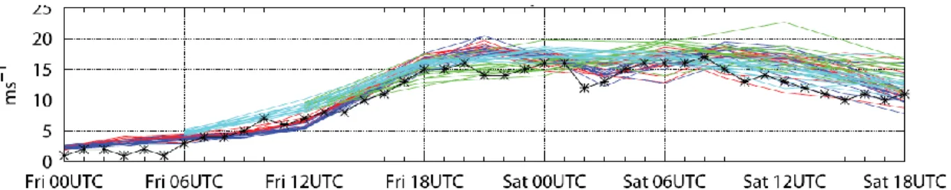
Examples of GLAMEPS forecasts are shown in Figure 6 which represents a meteogram collecting a series of runs of this model.

Figure 7: EPS-meteograms for the site 06235 De Kooy on the northwest coast of the Netherlands for an extreme weather case. The dates on the x-axes start on 29 February 2008 00UTC and end 42 h later, with 6 h between tick marks. Multicoloured curves on the bottom two diagrams are from the different model components of GLAMEPS EXP_0.2. Black curves with markers are observations. The curves show wind speed at a height of 10 m.

27

5 M ATHEM ATICAL FRAM EWO RK FOR DYNAM IC LINE RATING FORECASTING

An introduction to the mathematical framework of DLR forecast is presented here. As a reminder, DLR forecasts must be calculated for an entire line section or with a resolution up to the single span. Also, DLR forecast leadtime can be split into intraday forecasts (a few hours) and day-ahead forecasts, similar to other energy-related problems, which may involve different approaches.

Observations of raw ampacity may be available at temporal resolutions in the order of minutes, for instance from sag measurements post-processed with the meteorological conditions in the vicinity of the span. Let us denote by the raw ampacity reported at time t. In practice, for operational management decisions, the temporal resolution for the line rating forecast does not need to be too high. Time steps of 1-3 hours may be considered sufficient for operational purposes, but the dynamic thermal behaviour of the conductor must be taken into account at least for very short-term predictions (< 1h) as the typical time constant of a conductor is 10-20 min. In parallel, overhead line thermal rating is defined as a conservative estimate of the raw ampacity that may be observed within a time interval. Therefore typically for a time interval covering time steps from t-t to t, the minimum ampacity yt over that time interval is given as:

(7)

Other versions of this sampling procedure may be employed, i.e., more robust ones, in cases where it is suspected that outliers or poor-quality measurements may be present in the raw data reported. By applying this sampling procedure over the whole set of data available, the result is a time series of minimum ampacity for a span or line section of interest.

Since DLR forecasts give a conservative estimate of the ampacity of a span or line section, they may be naturally defined in a quantile forecasting framework. Indeed, when issuing a forecast at time t for lead time t+k, a quantile forecast with nominal proportion  is such that:

[ ̂ ] (8)

This means that there is only a probability  that the actual observed ampacity for the span or line is less than that forecast ̂ . By setting this nominal proportion at a sufficiently low level, say, 0.02, one may

then consider that the forecast gives a fairly safe minimum ampacity for the time interval index by t+k. Working with a quantile forecasting framework has the advantage that a number of time series and regression models exist that may be applied, inspired for instance by literature on probabilistic forecasting of wind power generation [89], or more generally literature on probabilistic forecasting in meteorology or economics.

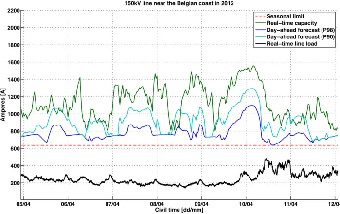
5.1 LINE CAPACITY FORECAST, EXAMPLE

DLR forecasts were calculated for the EU project TWENTIES, and in particular in the demonstration NETFLEX, for which the overhead line of the Belgian TSO ELIA was instrumented, with sag measurement units providing real-time ratings. During the project, line ampacity values were forecast for different time horizons up to 48 hours. Being able to forecast line capacity up to 2 days ahead is crucial to efficiently operate a flexible network and brings added value to DLR. Indeed, firmly forecast extra capacity can be directly used in today’s electricity market. In reality, essential core security calculations