HAL Id: hal-00916754
https://hal.archives-ouvertes.fr/hal-00916754
Submitted on 10 Dec 2013
HAL is a multi-disciplinary open access
archive for the deposit and dissemination of
sci-entific research documents, whether they are
pub-lished or not. The documents may come from
teaching and research institutions in France or
L’archive ouverte pluridisciplinaire HAL, est
destinée au dépôt et à la diffusion de documents
scientifiques de niveau recherche, publiés ou non,
émanant des établissements d’enseignement et de
recherche français ou étrangers, des laboratoires
Ray-Traced Collision Detection : Interpenetration
Control and Multi-GPU Performance
François Lehericey, Valérie Gouranton, Bruno Arnaldi
To cite this version:
François Lehericey, Valérie Gouranton, Bruno Arnaldi. Ray-Traced Collision Detection :
Interpenetration Control and MultiGPU Performance. 5th Joint Virtual Reality Conference of EuroVR
-EGVE, 2013, Paris, France. pp.1-8. �hal-00916754�
Joint Virtual Reality Conference of EGVE - EuroVR (2013) B. Mohler, B. Raffin, H. Saito, and O. Staadt (Editors)
Ray-Traced Collision Detection : Interpenetration Control
and Multi-GPU Performance
François Lehericey† Valérie Gouranton‡ Bruno Arnaldi§
INSA de Rennes, IRISA, Inria Campus de Beaulieu, 35042 Rennes cedex, France
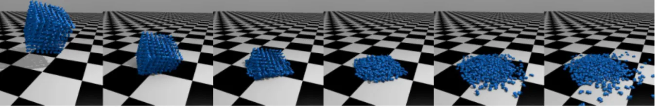
Figure 1: 512 concave mesh objects fall on a planar ground, up to 7300 pairs of objects are tested in the narrow phase. Abstract
We proposed in [LGA13] an iterative ray-traced collision detection algorithm (IRTCD) that exploits spatial and
temporal coherency and proved to be computationally efficient but at the price of some geometrical approximations that allow more interpenetration than needed. In this paper, we present two methods to efficiently control and reduce the interpenetration without noticeable computation overhead. The first method predicts the next potentially colliding vertices. These predictions are used to make our IRTCD algorithm more robust to the above-mentioned approximations, therefore reducing the errors up to 91%. We also present a ray re-projection algorithm that improves the physical response of ray-traced collision detection algorithm. This algorithm also reduces, up to 52%, the interpenetration between objects in a virtual environment. Our last contribution shows that our algorithm, when implemented on multi-GPUs architectures, is far faster.
Categories and Subject Descriptors(according to ACM CCS): I.3.1 [Computer Graphics]: Hardware Architecture—
Parallel processing I.3.5 [Computer Graphics]: Computational Geometry and Object Modeling—Physically based modeling
1. Introduction
In virtual reality (VR) and others applications of 3D environ-ments, collision detection (CD) is an essential task. Given a set of objects, those which might collide have to be known. Although this formulation is simple, collision detection is currently one of the main bottlenecks of VR application
be-† [email protected] ‡ [email protected] § [email protected]
cause of the real-time constraint imposed by the direct
inter-action of the user and the natural complexity (O(n2)) of the
naive algorithms. Recently, new approaches using GPGPU (General-Purpose computing on Graphic Processing Unit) have emerged while taking advantage of the GPU
compu-tational performances [AGA11].
In [LGA13] we presented an iterative ray-tracing algo-rithm for collision detection that uses spatial and tempo-ral coherency to improve performance. The main idea is to update when possible the result of the previous time step rather than computing new collisions from scratch. When
François Lehericey & Valérie Gouranton & Bruno Arnaldi / Interpenetration Control in Ray-Traced Collision Detection compared to non-iterative algorithms, the speedup obtained
with this algorithm is up to 33 times. Nevertheless, the main drawbacks of this method are: (1) it makes approximations when updating the collision and (2) the overall technique makes approximations on the direction of the physical re-action. These approximations may let the objects enter in further collision, increasing the total amount of interpene-tration in the virtual scenes.
In order to make this algorithm usable and efficient, we propose to control the interpenetration without loss of per-formances. This is performed using two methods that correct the approximations. The first one is a novel collision predic-tion method that predicts future collisions to reduce the er-rors when updating the previous result. The second one is a ray re-projection algorithm aiming at correcting the direc-tion of the physical reacdirec-tion.
We also propose to use multi-GPU architectures to exploit further the parallelization potential of the iterative and the predictive algorithm.
The paper is organized as follows: Section2presents the
related work. After a brief introduction of our previous
al-gorithm [LGA13], Section 3explains how we can reduce
the amount of interpenetration in the physics simulation with our predictive collision detection and re-projection
al-gorithms. Section4shows how we can use several GPUs to
improve the performances. Section5describes performance
improvements in our test scenes. Section6concludes this
paper and gives future work. 2. Related Work
In this section we focus on the literature of collision detec-tion that is the most relevant to our work. For a deeper in-troduction we suggest the reader to refer to surveys on the
topic [TKH∗05,KHI∗07]. Collision detection has to deal
with a large variety of objects and properties of these ob-jects. All these parameters can change the method used, and thus have created a lot of different solutions. Objects can be concave or convex, with or without holes. Objects can be solid, deformable, liquid and topology may change (they can split or merge). Objects can be represented with polyhe-drons (generally with triangular faces), CSG (Constructive Solid Geometry) or parametric functions.
Hubbard [Hub93] proposed to decompose collision
detec-tion in two phases, the broad-phase and the narrow-phase. The broad-phase plays the role of a filter by performing a cheap non-collision test to quickly remove non-colliding jects. The narrow-phase works with the pairs of objects ob-tained from the broad-phase. These pairs are in potential col-lision and the goal of the narrow-phase is to perform an exact collision test to give contact or interpenetration information so the physical response can be computed.
The broad-phase takes a set of objects as inputs and out-puts a set of potentially colliding pairs. Nowadays this phase
is less critical than the narrow-phase for performance. Aside brute force, broad-phase algorithms can be classified in three categories: spatial partitioning, kinematic and topology.
The narrow-phase takes the pairs produced by the broad-phase and performs an accurate collision test. It outputs a set of colliding objects and information about the contacts between objects for the physical response. Narrow-phase al-gorithms can be classified in four categories: feature-based, simplex-based, bounding volume hierarchy and image-based.
Nowadays GPUs (Graphics Processing Units) are broadly used to improve the performance of collision detection. [LHLK10] perform a massively parallel version of
sweep-and-prune algorithm on GPU for the broad-phase. [PKS10]
execute both broad and narrow phases on GPU and multi-GPU architectures with spacial subdivision.
2.1. Ray-Traced Collision Detection
Ray-Tracing Collision Detection Algorithms belong to the image-based category of narrow-phase algorithms. Several algorithms have been proposed in the literature. Wang and
al. [WFP12] launch rays from an irregular grid to
com-pute a layered depth image, the density of rays is higher around small objects to avoid missing them. Cinder
algo-rithm [Kno03] casts rays from the edges of an object and
counts how many object faces the ray passes through. If the result is odd then there is collision otherwise not. These rays are cast toward a regular grid.
Hermann and al. [HFR∗08] proposed to detect collision
by casting rays from the vertices of the objects. The algo-rithm is placed on the narrow-phase of the collision detec-tion pipeline and thus works on pair of potentially colliding objects. Rays are cast from each vertex of each object in the opposite direction of their normal. If a ray hits inside the other object before leaving the source object then a collision
is detected. Figure2shows an example. The plain arrows are
three rays that spot collision, the dotted arrow is a rejected ray because it hits the other object from outside.
Figure 2: Hermann and al. algorithm in 2D.
The main advantage of this algorithm is the information given for physical response. For other narrow-phase algo-rithms, when a collision is spotted additional computation is needed to compute the physical response. Hermann and al. algorithm gives for each penetrating vertex a direction and a
distance to separate the two objects (as can be seen in
Fig-ure2). The problem is, using the rays as is for the collision
response in the physical simulation gives incorrect behavior because the rays are not always correctly oriented to give a realistic physical response.
When using repulsion forces, Hermann and al. proposed an algorithm to weight the forces in order to reduce the tangential forces, but they are not suppressed. When using constraint-based response, weighting cannot be used as con-straint cannot be weighted. Furthermore to reduce the cost of constraint solver, contact-points reduction is applied on each colliding pair. After the reduction, the selected subset may contain only incorrectly oriented constraint. This will cause an incorrect physical response that can lead to accept further interpenetration by letting the objects sliding into each other. 3. Minimum Penetration Control
Based on Hermann et al. algorithm, we introduced in [LGA13] IRTCD: a new Iterative Ray-Traced Collision De-tection algorithm that is used to update the collision in a pair of objects when their relative displacement is inferior to a threshold displacementT hreshold. At each time step if the displacement exceeds the threshold we compute the rays with a standard algorithm (and reset the displacement to 0) otherwise we update the ray of the previous step with the iterative algorithm. The iterative algorithm relaunches the ray on the previously colliding triangles and iterates over the neighboring triangles until the new colliding ones are found. In this section we present how we reduce the total amount of interpenetration by making the detection and the physical
response better. Section3.1explains how we strengthen the
iterative algorithm with predictions. Section3.2shows how
we improve the physical response. 3.1. Predictive Collision Detection
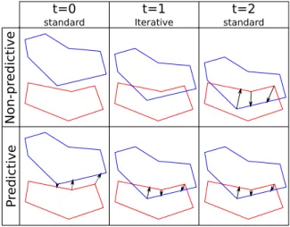
The main drawback of the iterative algorithm is it only works with previously detected rays. When new vertices enter in collision they will be taken into account only in the next standard step. This may postpone the collision detection of a pair of objects for several time steps, this will lead to
ac-cept further interpenetration. The first row of Figure3shows
an example of this situation. At t = 0 a standard algorithm is executed and no collision is detected. At t = 1 the previ-ous rays are updated, as the two objects were not colliding at t = 0 there are no rays to update. In this case the iterative algorithm fails to detect the collision. At t = 2 a standard algorithm is executed and the collision is detected. In this example the detection is postponed for only one step, but in practical cases it can be more.
We propose to solve this problem by performing a predic-tive ray/triangle intersection. When a ray does not detect any collision (and thus the corresponding vertex is not in colli-sion), we cast a predictive ray from the same vertex but in the
No n -p red ic ti v e P red ic ti v e t=0 standard t=1 Iterative t=2 standard
Figure 3: Comparison of predictive and non-predictive col-lision detection, with predictive rays the colcol-lision is detected earlier resulting in less interpenetration.
opposite direction. If this predictive ray hits a triangle and if the distance is short, the corresponding vertex may hit that triangle (or the neighboring ones) in a near future. Equation
1gives the distance from which we can cull the predictive
rays because the distance is too big. cullingDist depends on
displacementT hresholdand a confidence level of at least 1.
cullingDist= con f idence × displacementT hreshold (1)
The predictive rays are injected in the iterative
algo-rithm as candidates for the next steps. Algoalgo-rithm1 gives
the ray/triangle-mesh intersection algorithm that can han-dle prediction. The modification from the original algorithm [LGA13] is the addition of line 6 and 7. If the ray does not hit the current triangle, before looking at the neighboring tri-angle, we check if the current triangle is behind the ray. In such case the corresponding vertex is not in collision and the current triangle is kept as a candidate for the next step.
The second row of Figure3shows how these predictive
rays prevent delayed collision detection. At t = 0 a standard algorithm is executed and no collision is detected, predictive rays are cast outside the objects and three predictive rays kept. At t = 1 the predictive rays are updated and collision is successfully detected, at t = 2 a physical response can be applied to prevent further interpenetration.
We cast rays from the vertices that are inside the intersec-tion of the bounding volumes, this is an optimizaintersec-tion
pro-posed by [HFR∗08] to reduce the number of rays. In the
context of predictive rays this optimization may discard pre-dictive rays and delay the collision detection. To avoid this problem we extend the intersection of the bounding vol-umes by a distance of distanceExtension in all the directions
François Lehericey & Valérie Gouranton & Bruno Arnaldi / Interpenetration Control in Ray-Traced Collision Detection
Algorithm 1 Iterative ray/triangle-mesh intersection with
prediction handling
1: functionITRAYTRIINTERSEC(Ray ray, Triangle tri)
2: for i= 1 → maxIt do
3: intersection ←cast ray on tri
4: if rayhits tri then
5: return intersection
6: else if opposite(ray) hits tri then
7: return keepAsPrediction(tri)
8: else
9: edge ← closestEdge(tri, ray)
10: tri ← ad jacentTriangle(tri, edge)
11: end if
12: end for
13: return intertsectionNotFound
14: end function
which corresponds to a confidence zone. distanceExtension must be greater that displacementT hreshold, this ensures that we do not discard predictions that are essential for the iterative algorithm. The value of distanceExtension must be minimized for better performances because higher values in-crease the number of ray cast thus increasing computation.
In term of performance, casting a second ray in the oppo-site direction theoretically doubles the cost of the standard ray-tracing algorithm. In practical case we use two proper-ties to reduce the cost of the predictive rays. First the rays share several parameters in common, they have the same starting point and follow the same line (in the opposing di-rection). These shared parameters allow to factorize a por-tion of the two rays depending on the ray-tracing algorithm used. The second property is that we do not need to follow the predictive ray beyond the distance distanceExtension as it is exiting the confidence zone. This allows to shorten the ray traversal thus making it less expensive.
The evaluation of this predictive algorithm is given in
Sec-tions5.2and5.3.
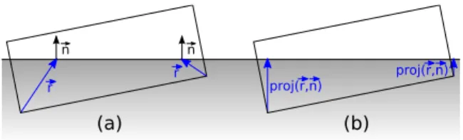
3.2. Ray Re-projection
With Hermann et al. algorithm, the orientation of the rays does not give the optimal direction for the physical response.
Figure4.a shows an example, the rays correctly detect the
collision but their directions do not correspond to the needs of the physical response (normal and tangential information)
shown in Figure4.b.
When executing the ray-tracing from the vertices, we record for each ray the normal of the impacted surface. Then we propose to post-process the rays by re-projecting them on the normal of the surface they collide. This re-projection minimizes the length of the rays. In physical simulation it corresponds to the Minimum Translational Distance (MTD)
[CC86], which is considered as a good heuristic for a
phys-ical collision response. An example of a ray re-projection is
shown in Figure4.b . (a) (b) n n r r proj(r,n) proj(r,n)
Figure 4: Collision between the box and the ground. In (a) the rays do not give the optimal separating direction. In (b) the rays have been re-projected on the normal of the surface they hit, these rays give the optimal collision response.
Projecting a ray on a vector can be done quickly with
Equation2, where ~r is the ray (the vector from the ray
ori-gin to the impacted point) and ~n is the unitary normal of the impacted surface.
pro j(~r,~n) = ~n × (~r ·~n) (2)
Collision response uses contact points to represent sion. A contact point is generally represented by one colli-sion point P with its penetration depth pd and its
separat-ing direction ~d(an example can be found in Figure5). With
this representation we can avoid to compute explicitly the re-projection of the ray with P = colliding vertex, pd =~r ·~n
and ~d= ~n.
This method makes no assumption on the physical re-sponse used and thus can be used with any physical rere-sponse algorithms.
P
d
pd
Figure 5: A contact point is composed of a point P, a
sepa-rating direction ~d and a penetration distance pd.
4. Adaptation for Multi-GPU Architectures
In [LGA13] we proposed to execute the iterative and stan-dard ray tracing algorithms on GPU to improve perfor-mance. GPU works with highly parallelized execution, we have to send to the GPU the work as an array of threads of several indices. We proposed to work with two indices.
The first index iterates through the pairs of objects from the broad-phase and each pair appears two times in opposite or-der. The second index iterates through the vertices of the first object of the pair, in each thread we cast the ray from the current vertex of the first object of the pair on the second object. This division on the work allows to parallelize the
ray-tracing by executing one ray cast per thread. Figure6
shows an example of such distribution.
ABBA ACCABDDBCDDCCE EC 1 2 3 4 5 6 pairs x,y i thver te x of x
Figure 6: Work distribution on one GPU. Each column cor-responds to a pair of objects, each row corcor-responds to a ver-tex of the first object of the pair. Filled squares are ray cast
from the ithvertex of x, white square are padding as each
object may have a different number of vertices.
We propose to exploit several GPUs to increase perfor-mance. To divide the work between the GPUs we break the first iteration into several blocks and execute these blocks on
different GPUs. Figure7gives an example with three GPUs.
The iterative algorithm uses at each step the result of the pre-vious step, this prepre-vious result is held in the memory of the GPU that proceed it. Memory transfers between two GPUs are expensive. To avoid transferring the previous result to another GPU we add a constraint: when a pair of objects is proceeded on one GPU, it must be processed on the same GPU until the pair is removed from de broad-phase.
ABBA ACCA 1 2 3 4 5 6 1 2 3 4 5 6 BDDBCD DCCE EC 1 2 3 4 5 6 ABBA ACCABDDBCDDCCE EC 1 2 3 4 5 6
Figure 7: Work distribution on several GPUs (three in this case). The iteration over the pairs is divided into several blocks that are assigned on different GPUs.
5. Performance Comparison
This section presents our experimental scenes and the result of our tests.
Section5.1presents our experimental scenes. Sections5.2
and5.3give the performances in term of detection and
com-putation time when our predictive algorithm is used.
Sec-tion5.4compares the physical response when our ray
re-projection algorithm is used. Section5.5gives the
perfor-mance improvements when using several GPUs. 5.1. Experimental Setup
We have tested our iterative ray-tracing collision detection algorithm with two different scenes. The first experimental scene is an avalanche of 512 concave meshes on a planar
ground (see Figure1), each mesh is composed of 453
ver-tices and 902 triangles. When the objects hit the ground, approximately 7300 pairs of objects are sent to the narrow-phase. The simulation is set to work at 60 Hz for 10
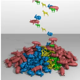
sec-onds. In the second experimental scene (see Figure8),
ob-jects are continually added in the scene at 10 Hz from a moving source that follows a circle. Four different concave meshes are used in equal quantity composed respectively of 902, 2130, 3456 and 3458 triangles. The simulation works at 60 Hz for 50 seconds. At the end 500 objects are present in the scene making a total count of approximately 1.2 million triangles in the scene and around 10,000 pairs of objects are sent to the narrow-phase in the last steps.
Figure 8: Second experimental scene, up to 10,000 pairs of objects are tested in the narrow-phase.
The experimental scenes were developed using Bullet
Physics (http://bulletphysics.org/). The
broad-phase and the physical response are executed on the CPU. Our narrow-phase algorithm was developed with OpenCL (http://www.khronos.org/opencl/) and can be executed on one or several GPUs. This setup generates mem-ory transfers between the CPU and the GPU as our algorithm is located in the middle of the physical simulation pipeline. In a real situation, the whole physical simulation pipeline would be implemented on GPU thus removing the memory transfers.
François Lehericey & Valérie Gouranton & Bruno Arnaldi / Interpenetration Control in Ray-Traced Collision Detection The iterative tracing algorithm needs a standard
ray-tracing algorithm as a starting point, we have implemented two algorithms:
Basic traversal:This algorithm does not use any
acceler-ation structure, for each ray we iterate through each triangle. This method has a high complexity but is simple.
Stackless BVH traversal:This algorithm uses a
bound-ing volume hierarchy (BVH) as an accelerative structure [WBS07] with a stackless traversal for GPUs [PGSS07]. This algorithm is more computationally efficient but has in-creased memory usage due to auxiliary data structures.
5.2. Predictive Detection Performances
To evaluate the importance of predictive rays, we run our two sample scenes with and without the predictive rays. Throughout the simulation we compare the results of the it-erative and itit-erative + predictive algorithms with a standard
ray-tracing algorithm used as a reference. Figures9and10
give the percentage of incorrect rays (i.e. when the result be-tween the standard and our algorithm is different). Results show a reduction up to 91% of the percentage of incorrect ray with the collision prediction algorithm.
0 0.02 0.04 0.06 0.08 0.1 0.12 0 1 2 3 4 5 6 7 8 9 10 In c o rrec t ra y s (p er c en ta g e) Time in simulation (s) Iterative Iterative + Predictive
Figure 9: Percentage of erroneous ray in the first scene.
To evaluate the impact of the predictive rays on the physics simulation we measure the cumulative length of all rays with a standard algorithm along the simulation, this value measures the amount of interpenetration in the whole scene. In the first scene the cumulative length of rays de-creases by 45% when using predictive rays. In the second scene we get a 56% decrease. This mean that the predictive rays effectively reduce the total amount of interpenetration.
5.3. Predictive Time Performances
To measure the impact on the computation time of predictive rays, we measure the time taken by the ray-tracing with and without the predictive ray with both ray-tracing algorithms.
0 0.02 0.04 0.06 0.08 0.1 0.12 0 5 10 15 20 25 30 35 40 45 50 In c o rrec t ra y s (p er c en ta g e) Time in simulation (s) Iterative Iterative + Predictive
Figure 10: Percentage of erroneous ray in the second scene.
Figures11and12show the time spent on ray-tracing along
the simulation for each scene on a Nvidia GTX 660. When the iterative algorithm is used (e.g., part C of
Fig-ure11), the usage of predictive rays has a small impact on
the computation time. This is because the casting of the pre-dictive ray in the iterative algorithm can be factorized with the casting of the standard ray, resulting in a low overhead.
When there is less spatial and temporal coherency and the standard ray-tracing algorithm is intensely used (e.g., B of
Figure11), the impact on the computation time of the
pre-dictive rays depends on the ray-tracing algorithm used. With the basic traversal we can completely factorize the casting of the predictive with the standard ray to avoid traversing the object twice. This makes the cost of the pre-dictive ray negligible. In parallel the usage of prepre-dictive rays reduces the amount of interpenetration in the scene which re-duces the number of collision and consequently rere-duces the number of rays to compute. Finally the cost of casting the predictive rays is lower the gain we have by decreasing the number of rays to compute. This result can be seen in part B
of Figure11where we have an average 1.27 speedup.
With the stackless BVH traversal we cannot factorize the traversing of the predictive ray with the standard ray. But we can limit the traversal of the BVH by limiting the ray length
to a maximum of cullingDist as explained in Section3.1
to avoid doubling the cost of the standard algorithm. In our experimental scenes, the worst speedup we have by adding predictive ray to the stackless is an average of 0.78 in part B
of Figure11.
These results show that the computational cost of using the re-projection algorithm is low, in the worst case we have a 0.78 speedup and in the best case we have a 1.27 speedup. 5.4. Ray Re-projection Performances
As a test we can consider the case of an object in collision with the ground, in such case the reaction should be
0 10 20 30 40 50 60 70 0 1 2 3 4 5 6 7 8 9 10 Co mp u ta ti o n ti me (ms ) Time in simulation (s) A B C
iterative basic traversal iterative basic traversal + predictive iterative stackless BVH traversal iterative stackless BVH traversal + predictive
Figure 11: Time spent executing ray-tracing with and with-out predictive rays in the first scene.
0 20 40 60 80 100 120 140 50 100 150 200 250 300 350 400 450 500 Co mp u ta ti o n ti me (ms )
Number of objects in the scene iterative basic traversal
iterative basic traversal + predictive iterative stackless BVH traversal iterative stackless BVH traversal + predictive
Figure 12: Time spent executing ray-tracing with and with-out predictive rays in the second scene.
onal to the ground. This test has been proposed by Hermann
et al. [HFR∗08] for evaluating their weighting algorithm. We
have tested three objects: a discretized sphere and two irreg-ular shapes. Each object has been tested with 400 different orientations and 20 different interpenetration depths (as
il-lustrated in Figure13). Table1gives the average deviation
defined as the ratio of the tangential and normal forces, in theory this deviation should be zero.
Figure 13: To test the average deviation of the reaction of an object and the ground, we perform the collision detection with several interpenetration distance and orientations.
Technique sphere bunny pig
Number of vertices 70 453 1085
Standard 3.97 22.0 27.0
Weighting [HFR∗08] 2.66 16.5 20.6
Re-projection 0.00 0.00 0.00
Table 1: Average deviation of penalty forces in percent for three meshes against the ground.
The deviation of the forces with the sphere is low. This can be explained by the regularity of the shape. Due to the symmetry, the forces balance with each other. With irregu-lar objects forces do not balance as well and deviation is not negligible. The weighting technique proposed by Hermann et al. reduces the tangential forces, but it only reduces the de-viation by about 25% for irregular shapes. Our re-projection technique guarantees a 0% deviation as the forces are reori-ented toward the optimal direction.
We have tested our re-projection algorithm with our two experimental scenes, the collision response is managed with a sequential impulse solvers with contact-points reduc-tion. We perform the simulation with and without ray re-projection and measure the total length of the rays along the simulation as a global interpenetration measurement. Table
2gives the cumulative length of all rays for both scenes with
and without ray re-projection and the decrease percentage. Results shows that our solution effectively reduces the total interpenetration, up to 59%.
Standard Re-projection Decrease
Scene 1 16 115 10 793 59%
Scene 2 66 094 38 398 42%
Table 2: Comparison of the cumulative length of all rays along the simulation with and without ray re-projection.
5.5. Multi-GPU Performances
We run our experimental scene with the iterative ray-tracing algorithms on one Nvidia GTX 580 and on multi-GPU setup
of two Nvidia GTX 580. Figures14and15show the time
spent on ray-tracing on the GPU at each simulation step for each scene. With two GPUs, we get an average speedup of 1.77 and 1.66 for respectively the first and second scene. 6. Conclusion and Future Work
In the context of iterative ray-tracing for collision detection, our collision prediction algorithm avoids to miss new col-lision when the iterative ray-tracing algorithm is used. Re-sults show a reduction of the total interpenetration in our test scenes up to 56% with our collision prediction algorithm. We also presented a ray-reprojection algorithm to improve the
François Lehericey & Valérie Gouranton & Bruno Arnaldi / Interpenetration Control in Ray-Traced Collision Detection 0 1 2 3 4 5 6 7 8 9 0 1 2 3 4 5 6 7 8 9 10 Co mp u ta ti o n ti me (ms ) Time in simulation (s) One GPU Two GPU
Figure 14: Time spent executing ray-tracing on one and two Nvidia GTX 580 in the first scene.
0 2 4 6 8 10 12 50 100 150 200 250 300 350 400 450 500 Co mp u ta ti o n ti me (ms )
Number of objects in the scene One GPU Two GPU
Figure 15: Time spent executing ray-tracing on one and two Nvidia GTX 580 in the second scene.
collision response. Total interpenetration in our test scenes has been reduced up to 52%. We have presented an adapta-tion for multi-GPU architectures that gives a speedup up to 1.77 with two GPUs.
In our methods we have three constants along the simula-tion: maxIt and displacementT hreshold that comes from the iterative ray-tracing algorithm, and distanceExtension that come from the collision prediction algorithm. Their values depend on the object sizes and velocities in the scene. In fu-ture work it would be interesting to study more deeply the impact of the choice of these values on the simulation and to try to use dynamics values instead of constants in order to optimize these values along the simulation.
We also want to study the multi-GPU scalability of our al-gorithm when using many GPUs to be able to simulate more complex scenes.
It also would be interesting to extend our algorithm to de-formable bodies. With rigid bodies we can use accelerative ray-tracing structure with a high construction cost. In the
case of deformable bodies the ray-tracing accelerative struc-ture needs to be updated at each time step making complex ray-tracing techniques more expensive. In addition self colli-sion has to be detected. We believe that our iterative, predic-tive and re-projection algorithms are suitable for deformable bodies and should improve the performance of ray-tracing collision detection algorithms for deformable bodies. References
[AGA11] AVRILQ., GOURANTONV., ARNALDIB.: Dynamic adaptation of broad phase collision detection algorithms. In VR Innovation (ISVRI), 2011 IEEE International Symposium on (2011), IEEE, pp. 41–47.1
[CC86] CAMERONS., CULLEYR.: Determining the minimum translational distance between two convex polyhedra. In Robotics and Automation. Proceedings. 1986 IEEE International Confer-ence on(1986), vol. 3, IEEE, pp. 591–596.4
[HFR∗08] HERMANNE., FAUREF., RAFFINB.,ET AL.:
Ray-traced collision detection for deformable bodies. In 3rd Interna-tional Conference on Computer Graphics Theory and Applica-tions, GRAPP 2008(2008).2,3,7
[Hub93] HUBBARDP.: Interactive collision detection. In Virtual Reality, 1993. Proceedings., IEEE 1993 Symposium on Research Frontiers in(1993), IEEE, pp. 24–31.2
[KHI∗07] KOCKARA S., HALIC T., IQBAL K., BAYRAK C.,
ROWE R.: Collision detection: A survey. In Systems, Man and Cybernetics, 2007. ISIC. IEEE International Conference on (2007), IEEE, pp. 4046–4051.2
[Kno03] KNOTTD.: Cinder: Collision and interference detection in real–time using graphics hardware.2
[LGA13] LEHERICEYF., GOURANTONV., ARNALDIB.: New iterative ray-traced collision detection algorithm for gpu archi-tectures. In Proceedings of the 19th ACM Symposium on Virtual Reality Software and Technology(2013), ACM, pp. 215–218.1,
2,3,4
[LHLK10] LIUF., HARADAT., LEEY., KIMY. J.: Real-time collision culling of a million bodies on graphics processing units. In ACM Transactions on Graphics (TOG) (2010), vol. 29, ACM, p. 154.2
[PGSS07] POPOVS., GÜNTHERJ., SEIDELH.-P., SLUSALLEK
P.: Stackless kd-tree traversal for high performance gpu ray trac-ing. In Computer Graphics Forum (2007), vol. 26, Wiley Online Library, pp. 415–424.6
[PKS10] PABSTS., KOCHA., STRASSERW.: Fast and scalable cpu/gpu collision detection for rigid and deformable surfaces. In Computer Graphics Forum(2010), vol. 29, Wiley Online Library, pp. 1605–1612.2
[TKH∗05] TESCHNERM., KIMMERLES., HEIDELBERGERB.,
ZACHMANN G., RAGHUPATHI L., FUHRMANN A., CANI
M., FAURE F., MAGNENAT-THALMANN N., STRASSERW.,
ET AL.: Collision detection for deformable objects. In Computer Graphics Forum(2005), vol. 24, Wiley Online Library, pp. 61– 81.2
[WBS07] WALDI., BOULOSS., SHIRLEYP.: Ray tracing de-formable scenes using dynamic bounding volume hierarchies. ACM Transactions on Graphics (TOG) 26, 1 (2007), 6.6 [WFP12] WANGB., FAUREF., PAID.: Adaptive image-based
intersection volume. ACM Transactions on Graphics (TOG) 31, 4 (2012), 97.2