A node-nested Galerkin multigrid method for metal forging simulation

HAL Id: hal-00581743

https://hal-mines-paristech.archives-ouvertes.fr/hal-00581743

Submitted on 31 Mar 2011

HAL is a multi-disciplinary open access archive for the deposit and dissemination of sci-entific research documents, whether they are pub-lished or not. The documents may come from teaching and research institutions in France or abroad, or from public or private research centers.

L’archive ouverte pluridisciplinaire HAL, est destinée au dépôt et à la diffusion de documents scientifiques de niveau recherche, publiés ou non, émanant des établissements d’enseignement et de recherche français ou étrangers, des laboratoires publics ou privés.

A node-nested Galerkin multigrid method for metal

forging simulation

Benoît Rey, Katia Mocellin, Lionel Fourment

To cite this version:

Benoît Rey, Katia Mocellin, Lionel Fourment. A node-nested Galerkin multigrid method for metal forging simulation. EMG 2005 - Multigrid, Multilevel and Multiscale Methods, Sep 2005, Delft, Netherlands. 10 p. - ISBN 90-9020969-7. �hal-00581743�

A node-nested Galerkin multigrid method for metal forging simulation

B. Rey*, K. Mocellin, L. Fourment

CEMEF, Ecole des mines de Paris, BP 207, 06904 Sophia Antipolis, France E-mail address: benoit.rey@ensmp.fr

Abstract :

A node-nested Galerkin multigrid method is developed to solve systems provided by mixed formulations of 3D metal forming problems. An algebraic approach is used where operators are built on node-nested coarse meshes obtained by an automatic coarsening algorithm. This blackbox multigrid preconditioner is developed within the PETSc library. It is plugged to the FORGE3® finite element software. The linear rate of convergence and the very high efficiency of the resulting multigrid solver are evaluated for large scale problems with non-linear behaviour.

Keywords: algebraic multigrid, mixed formulation, finite element method, 3D metal forming,

mesh coarsening, node-nested meshes, automatic remeshing

1. Introduction

This work is motivated by the success of the finite element methods for solving three dimensional metal forming problems at industrial scale. However, the constant need for more accuracy and reliability of the computations result in smarter spatial discretization that cannot be only made available by more powerful computers. In fact, reducing the mesh size by a factor of 2 in each space direction in 3D, which is not much, results into an increase of the number of nodes by a factor 8. As at least 75% of the computational time of a finite element simulation is spent for the resolution of linear systems, using an iterative solver which computational cost is proportional to N3/2 (N being the number of degrees of freedom), this reduction will result into an increase of computational time by about a factor of 20. This shows the need to reduce the computational cost of systems resolution and more particularly its dependency to the number of degrees of freedom, independently on the increase of the computers power. Therefore, solver with a linear rate of convergence is quite an attractive solution. Multigrid method is known to be efficient for solving systems derived from finite element problems [1]. As discussed in [2], multi-scale strategies have the unique potential of solving most of the mathematical problems with N unknowns in O(N) works. This paper discusses the implementation of a multigrid solver into the Forge3® F.E. software that is dedicated to 3D thermo-mechanical forging simulation.

2. Forging simulation problem

More details on Forge3® model are available in [3]. For simplicity, the problem equations are presented under hot forging conditions when the elastic deformations can be neglected and the material assumed to be homogenous, isotropic and incompressible. The mechanical problem consists in the equilibrium equation, where inertia and gravity contributions can be neglected, and the incompressibility equation:

⎩ ⎨ ⎧ Ω = Ω = in 0 div in 0 div v σ (1)

where Ω is a time dependant domain, σ the stress tensor and v the velocity. This couple of equations has to be completed with boundary conditions where the boundary of domain Ω is decomposed into: ∂Ω=∂Ω_C ∪∂Ω_F; ∂Ω_C is the contact surface with forming tools and ∂Ω_F is the free surface :

(

)

(

)

[

]

⎪ ⎪ ⎪ ⎩ ⎪ ⎪ ⎪ ⎨ ⎧ Ω ∂ = − Ω ∂ ≤ Ω ∂ ≤ − Ω ∂ = Ω ∂ ∆ ∆ − = − C n die C n C die F c s q s f n v v n v v n v v K on 0 . on 0 on 0 . on 0 on 1 σ σ σ α τ (2)

The friction power law gives the tangent shear stress τ at the workpiece/tool interface as a function of the relative tangent velocity ∆v_s defined by:

(

)

[

v v n

]

n v v v_s = − _die− − _die . ∆ (3) f

α is a friction coefficient, K the material consistency, and q a sensitivity coefficient. v_die

denotes the velocity of the die and n the outside normal to the workpiece.

The second equality of (2) is the free surface condition. The last three equations of (2) are the Signorini conditions, which denote the unilateral contact condition and the non-penetration condition of the workpiece into the tools. The contact pressure σ_n is defined by:

n n

n σ .

σ = (4)

The constitutive law of the material is regarded as viscoplastic. The Norton-Hoff law is considered here:

( )

ε ε

σ +pI =2K 3& m−1& (5)

where p is the hydrostatic pressure, I the identity tensor, ε& the equivalent strain rate, m the

viscoplasticity coefficient and ε& the strain rate tensor.

Invoking the virtual work principle, a weak formulation of the mechanical problem formulated in terms of velocity and pressure is obtained. Tetrahedra and a P1+/P1 mini element mixed interpolation are selected to discretize the problem. First introduced in [4] this interpolation ensures the stability condition (Brezzi Babuska condition) by enriching the linear velocity field with a bubble function at the center of the element.

The unilateral contact condition is enforced to finite element nodes by a penalty method, so the additional penalty terms that appear in the system matrix are located on its block diagonal. The resulting nonlinear set of equations is solved by a Newton-Raphson algorithm. In the

linear case (m= q=1), the mini-element interpolation provides a discrete linear system to

solve that has the following matrix form:

⎟ ⎟ ⎟ ⎠ ⎞ ⎜ ⎜ ⎜ ⎝ ⎛ = ⎟ ⎟ ⎟ ⎠ ⎞ ⎜ ⎜ ⎜ ⎝ ⎛ ∆ ∆ ∆ ⎟ ⎟ ⎟ ⎠ ⎞ ⎜ ⎜ ⎜ ⎝ ⎛ p b v b T b T b b R R R P V V B B B H B H 0 0 0 (6)

where ∆V and P∆ respectively are the nodal vector corrections to the initial values of the

velocities and pressure, and ∆ is the velocity bubble contribution at the center of the V_b

elements.

The internal velocity bubble terms are eliminated from the equations by static condensation,

b b T bH B B C= −1 (7)

The remaining linear parts of the correction of the velocity and pressure are then solution of the following system:

⎟⎟⎠ ⎞ ⎜⎜⎝ ⎛ − = ⎟⎟⎠ ⎞ ⎜⎜⎝ ⎛ ∆ ∆ ⎟⎟⎠ ⎞ ⎜⎜⎝ ⎛ − − b b T b p v T _{R B H R} R P V C B B H 1 (8)

where H and C are both symmetric positive definite, so that the global matrix of the system

is not definite.

The system unknowns are the three velocity components and the pressure for each node of the finite element mesh: the number of degrees of freedom (dof) of the system equals four times the number of nodes. This linear system is usually solved by a preconditioned conjugate residual method (PCR), where preconditioning is performed by an incomplete Cholesky factorization. This reference preconditioner is replaced by the multigrid method in the present work and more precisely by a single iteration of a multigrid V-cycle, as in [5].

3. Multigrid 3.1. Notations

The algebraic multigrid approach [6] is used to compute the coarse matrix, so it is defined by the Galerkin strategy:

P RA

A_coarse = _fine (9)

The Ritz-Galerkin strategy is also selected:

T

R

P= (10)

The coarsest grid correction is compute by a direct solver that uses LU factorization.

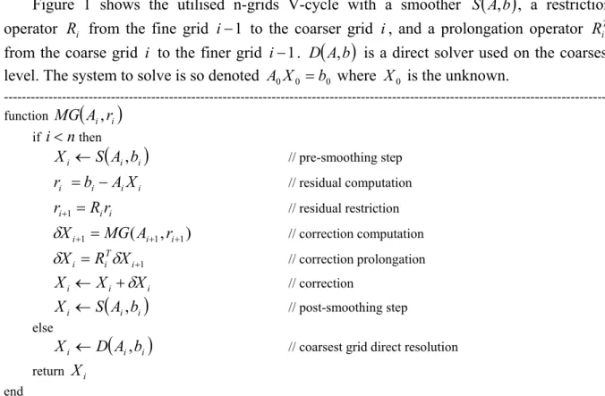
Figure 1 shows the utilised n-grids V-cycle with a smoother S

( )

A,b , a restriction

operator R_i from the fine grid i−1 to the coarser grid i , and a prolongation operator R_iT

from the coarse grid i to the finer grid i−1. D

( )

A,b is a direct solver used on the coarsest

level. The system to solve is so denoted A₀X₀ = where b₀ X₀ is the unknown.

--- function MG

(

A_i,r_i

)

if i<nthen

(

i i

)

i S A b X ← , // pre-smoothing step i i i i b AX r = − // residual computation i i i Rr r₊₁= // residual restriction ) , ( _{1 1} 1 + + + = i i i MG A r X δ // correction computation 1 + = i T i i R X X δ δ // correction prolongation i i i X X X ← +δ // correction

(

i i

)

i S A b X ← , // post-smoothing step else

(

i i

)

i D A b

X ← , // coarsest grid direct resolution

return X_i

end

---fig. 1: Multigrid V-cycle algorithm

3.2. Automatic coarse grid creation

According to equation (10), only the restriction operators need to be evaluated. It is done following a geometrical approach by constructing different levels of meshes of smaller number of element. Therefore the main issue is to build coarse meshes.

The use of an element-nested method as in [7] is prohibited because the remeshing issue requires a fully automatic procedure to generate the different levels of meshes. The use of a non-nested meshes as in [8] is also leave behind because the R and P operators are more complex to build and more expensive to use than in a node-nested method. Therefore this node-nested method is preferred here.

For a 2D geometry, Guillard [9] and independently Chan and Smith [10] proposed a Maximal Independent Subset (MIS) algorithm to compute coarse meshes from fine ones. Adams [11] proposed a 3D extension of these algorithms but another technique [12] is prefered here to compute coarse meshes. It is based on an iterative node removal algorithm combined to a local remeshing algorithm, with almost constant coarsening ratio. This automatic coarsening technique is part of the MTC® mesh generator toolbox [13].

h

M is defined by its set of nodes I_h and its set of tetrahedra T_h. For any node i∈ , the I_h

average length l_h

( )

i of the edges connected to i is computed. Ideally, in the coarse mesh

extracted from M_h, for any i∈I_H the length l_H

( )

i of the edges will be

( )

C i l_h

, where C is the

targeted average length ratio which is usually chosen equal to 2 for an isotropic mesh. The

aim of the algorithm is to build a coarse mesh where the average length l_H

( )

i of any node i

has the targeted value. Let CR be the coarsening ratio that is equal to the number of nodes of

the initial mesh divided by the number of nodes of the coarse one.

Let T

( )

i be the set of tetrahedra that contains the node i , ε

( )

i be the set of nodes of T

( )

i

(not including i ) and F

( )

i be the set of exterior faces of T

( )

i (that do not contain i ). The

removal of nodes is carried out by the algorithm described in figure 2.

---1. for any node i, compute l_H

( )

i

2. do M_current =M_h: T_current =T_h and I_current = I_h

3. for any node i in I_current, compute l_current

( )

i the average length of edges connected to i

4. if l_current

( )

i ≥l_H

( )

i then 1 + ← i i and go to 3 else

• remesh the volume defined by F_current

( )

i using only nodes of ε_current

( )

i , let T_new

( )

i be the set of tetrahedra of this new triangulation

• if T_new

( )

i is acceptable then

o I I

{}

i current current = − o T T T

( )

i T

( )

i new current current = − + o i← i+1 _{and go to 3} else o i← i+1 _{and go to 3}

5. M_H =M_current:T_H =T_current and I_H =I_current

---fig. 2: coarsening algorithm

The remeshing of the cavity in step 4 of figure 2 produced by removing node i , described in figure 3, is carried out by successively exploring all possible triangulations made by

connecting a node of ε

( )

i to all faces of F

( )

i . Among all these triangulations, only the ones

which volume almost equals the volume of F

( )

i are kept and the one with the best element

quality is selected.

fig. 3: cavity remeshing

This way the coarse meshes are node-nested with the initial one. Figure 4 show examples of coarse meshes obtained with this algorithm in the cases of a connecting rod and a ring at a certain stage of the forming process.

40,897 nodes 4,857 nodes

Fig. 4: fine and coarse meshes of a connecting rod (coarsening ratio: 8.4)

In fact, the construction of coarse mesh is not as straight forward as it may seem from these examples, because the coarse mesh has to satisfy the geometrical constraint of properly representing the shape of the domain. Therefore, in order to obtain a satisfactory fully connex mesh with no significant volume or shape alteration, it is necessary to reduce the expectation in terms of coarsening ratio. For more complex geometries, as encountered at the end of forging, it is then difficult to obtain a coarse mesh with sufficiently small number of nodes, which can penalize the multigrid efficiency because of the computational cost of the direct system resolution on the coarsest level.

3.3. Operators computation

The restriction operator, is obtained by a linear interpolation of fine nodes values onto coarse nodes. Figure 5 describes the linear dependencies in a 2D case. For any node i , the

coarse element

(

j₁,j₂,j₃

)

that contains i is found and its barycentric coordinates are

calculated. If the fine node is also a coarse one, there is only one non-zero value its row. Otherwise, there are only four non-zero values its row.

fig. 5: interpolation of fine nodes values onto the nodes of a coarse element

With the used of Lagrangian formulation, the mesh endures large deformations during simulation. This deformation is not linear, so the barycentric coordinates of fine nodes with respect to the coarse mesh change. However, for simplicity these changes are not taken into account and operators are assumed to be constant. In [7], it has been observed that this approximation does not reduce the efficiency of the multigrid method with the material deformation.

3.4. Other multigrid components

The multigrid method is used as a preconditioner for the conjugate residual solver. This new preconditioned solver is developed within the PETSc library, which still need to be provided by coarse meshes, restriction operators and adequate numerical parameters.

In this frame, several smoothers available in PETSc have been tested. Block Jacobi has been selected because it offers the best compromise between high frequency smoothing and low computational cost.

The coarsest grid correction is calculated by direct resolution. Experience shows that the direct solver is regarded as the quickest when the number of dof is less than 6,000, i.e. when the coarsest mesh contains less than 1,500 nodes. Habitual meshes used for standard forging simulations contain between 10,000 and 80,000 nodes so three different levels with a coarsening ratio of 8 approximately each, are necessary and sufficient to obtain an efficient method where the coarsest mesh resolution can be direct. This is why all our numerical results have been obtained with a three levels method.

The number of pre and post smoothing steps are fit by a parametric study on a typical forging problem. Best results are obtained with one smoothing and one post smoothing iteration. It both minimizes the total number of smoothing steps and the computational time of the resolution.

4. Numerical results

This section investigates the performances of the developed three levels multigrid method (MG3). First of all the linear rate of convergence of the solver is verified. Then the performances are compared to the reference preconditioned conjugate residual solver (CR/ILU), the same convergence criterion being used for both methods.

4.1. Linear rate of convergence

The evolution of the computational time resolution is observed for various systems provided by the connecting rod forming at the end of the simulation (non linear material behaviour and friction coefficient equals 0.14). The different used meshes have 11,245 nodes, 31,200 nodes, 47,083 nodes, 61,987 nodes and 91,127 nodes. The left curve of figure 6 shows the evolution of the resolution time with CR/ILU (plain line) and MG3 (dotted line) solvers.

Comparing the resolution time of the two methods for the same system, the larger the number of dof is, the more the speed-up provided by MG3 is relevant. The gain is effective when the mesh contains more than 10,000 nodes.

The multigrid solver is close to its optimal linear rate of convergence O

( )

n , where n is

the number of unknowns: see figure 6 right, where the black line corresponds to a perfect linear behavior and the dotted line to the MG3 rate of convergence.

resolution time of a linear system

0 200 400 600 800 1000 1200 0 10000 20000 30000 40000 50000 60000 70000 80000 90000 100000 number of nodes c pu t im e ( s e c ond) MG3 CR / ILU

linear complexity of the multigrid method

0 20 40 60 80 100 120 0 10000 20000 30000 40000 50000 60000 70000 80000 90000 100000 number of nodes c pu t im e ( s e c ond) MG3 Linéaire (MG3)

Fig. 6: computational cost of the multigrid and CR/ILU solver as a function of dof

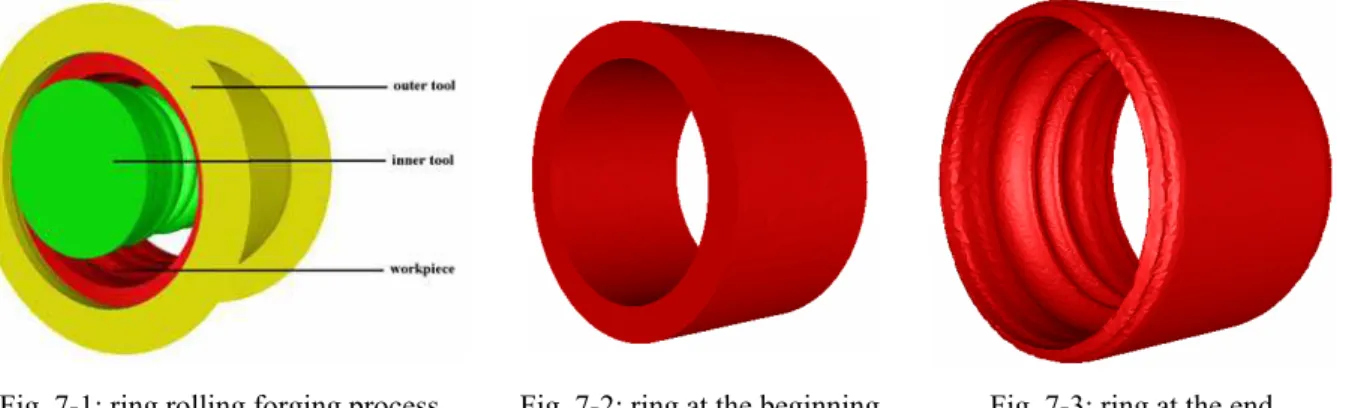
4.2. Application to the simulation of the ring rolling process

The efficiency of the multigrid solver is now evaluated for a complex forging simulation, the forming of an external ring of a ball bearing system. Figure 7-1 shows the process with the outer die, the workpiece and the inner die, which has an excentric circular movement. Figure 7-2 shows the workpiece at the beginning and figure 7-3 at the end of the process. The viscoplasticity coefficient is 0.1529, the material has a consistency of 2707 MPa and a temperature of 700°C. Contact between workpiece and tools is supposed to be perfectly sliding.

Fig. 7-1: ring rolling forging process Fig. 7-2: ring at the beginning Fig. 7-3: ring at the end

During the whole simulation, 44 remeshing steps are necessary. Every time a remeshing is done, new coarse meshes are automatically created for the three levels method. The simulation has been entirely carried out with the multigrid solver, without any external intervention. For discussion, only the calculation time of the first three time increments is studied. It includes the two coarse meshes construction using the coarsening algorithm, the calculation of the restriction operators and of the coarse matrices.

The three studied simulations regard meshes with respectively 11,245 nodes, 31,200 nodes and 61,987 nodes. Table 1 summarizes the data of the computational and different coarse meshes used by the multigrid method.

Number of dof of the

simulation 44,980 124,800 247,948

Number of nodes of the

computation mesh 11,245 31,200 61,987

Number of nodes of the

intermediate mesh 1,452 3,233 6,061

Number of nodes of the

coarse mesh 189 509 790

Tab. 1: number of nodes of the different meshes

Figure 8 shows the different meshes used for the 31,200 nodes simulation. The computational mesh is on the left hand side. In the centre, the intermediate mesh is showed, and on the right hand side the coarse mesh.

31,200 nodes 3,233 nodes 509 nodes

Fig. 8: computational, intermediate and coarse meshes for the 124,800 dof simulation

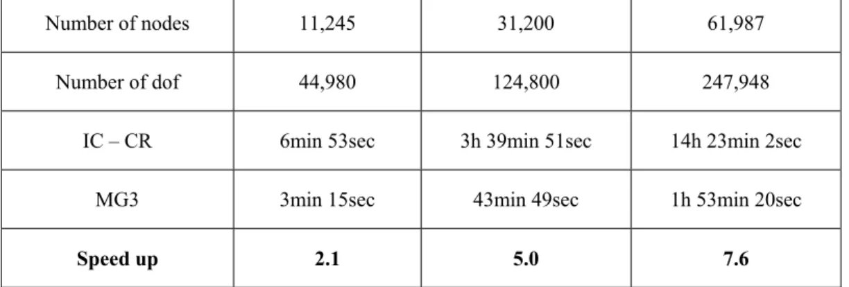
Table 2 summarizes the obtained calculation times. The speed up observed with the multigrid solver directly depends on the mesh size. For 44,980 dof the calculation time is reduced by 2.1. On a more substantial example, with 247,958 dof, the recorded speed up is 7.6 and the time saving is about 12h. These performances are really interesting and provide a considerable minimisation of calculation time for numerical simulations.

Number of nodes 11,245 31,200 61,987

Number of dof 44,980 124,800 247,948

IC – CR 6min 53sec 3h 39min 51sec 14h 23min 2sec

MG3 3min 15sec 43min 49sec 1h 53min 20sec

Speed up 2.1 5.0 7.6

Table 2: CPU time and speed up of the first three time increment of simulation

5. Conclusion

A node-nested Galerkin multigrid method has been developed for solving linear system derived from 3D forging simulations with a mixed finite element formulation. This method is plugged to Forge3® software and remains see-through for the user. Moreover, it is compatible with frequent remeshings and with the mixed velocity-pressure formulation. A standard algebraic method might encounter difficulties with the contact penalty terms of the system matrix, while the used mixed algebraic / geometric approach avoids it. An automatic

coarsening technique allows computing the various coarse meshes required by the construction of the transfer operators. The node-nested characteristic provides sparse and simple interpolation and restriction passing matrices. The construction of a coarse system by the Galerkin relation is not time consuming. Operators are considered to be constant between two remeshing steps, and even if these steps do not occur frequently, no decrease of performances is observed because of this approximation. When the domain is too complex it is not always possible to build coarse meshes with a coarsening ratio close to 8, but the method has showed to be quite robust when applied to an entire ring rolling simulation with 44 remeshing steps.

This multigrid solver shows a promising global reduction of the computational time. It is also more robust that the previously used solver. Some more forging simulations have been carried out to extend these conclusions to other problems. The speed-up and the robustness of the multigrid solver were not denied. The linear asymptotic convergence rate has been noticed in the particular studied frame of a mixed velocity - pressure formulation.

These first results are really encouraging and confirm that the use of the multigrid is advised for large scale simulations. First improvements are currently "taking place". An iterative resolution method is currently tested to solve the coarsest system when the coarsest mesh contains too many nodes. Therefore, if the coarsening technique does not allow obtaining a sufficiently coarse mesh, an iterative solver will provide a less expensive solution than a direct solving. Future works will deal with the study of larger problems with several bodies, where the number of dof will grow up, so the use of the multigrid method will be even more justified. The solver will also have to be adapted to parallel computation using a SPMP strategy with dynamic mesh partionning.

References

[1] Okasanya T., Darmofal D.L., Peraire J.: Algebraic multigrid for stabilized finite element discretizations of the Navier-Stokes equations. Computer Methods in Applied Mechanics and Engineering 193, pp.3667-3686, 2004

[2] Brandt A.: The Gauss Center research in multiscale scientific computation. Electronic Transactions on numerical Analysis vol. 6, pp. 1-34, 1997

[3] Chenot J. L.: Three dimentional finite element modeling of forging process. Computational Plasticity, Pienridge press, pp. 793-816, Swansea, 1989

[4] Arnold D. N., Brezzi F., Fortin M.: A stable finite element for Stokes equations. Calcolo, 21, pp. 337-344, 1984

[5] Iwamura C., Costa F. S., Sbarski I., Easton A., Li N.: An efficient algebraic multigrid preconditioned conjugate gradient solver. Computer Methods in Applied Mechanics and Engineering 192, pp. 2299-2318, 2003

[6] Strüben K.: A review of algebraic multigrid. Journal of Computational and Applied Mathematics 125, pp. 281-309, 2001

[7] Coupez T., Mocellin K., Fourment L., Chenot J.-L.: Toward large scale F.E. computation of hot forging process using iterative solvers, parallel computation and multigrid algorithms. International Journal for Numerical Methods in Engineering 52, pp. 473-488, 2001

[8] Feng Y.T., Peric D., Owen D.R.J.: A non-nested Galerkin multigrid method for solving linear and nonlinear solid mechanics problems. Computer Methods in Applied Mechanics and Engineering 144, pp. 307-325, 1997

[9] Guillard, H.: Node-nested multigrid method with Delaunay coarsening. INRIA TechReport No1898, 1993

[10] Chan T.,Smith B.: Domain decomposition and multigrid algorithms for elliptic problems unstructured meshes. Electronic Transactions in Numerical Analysis, 2, pp. 171-182, 1994

[11] Adams M., Taylor R.L.: Parallel multigrid solvers for 3D-unstructured large deformation elasticity and plasticity finite element problems. Finite Element in Analysis and Design 36 pp. 197-214, 2000

[12] Carte G., Coupez T., Guillard H., Lanteri S.: Coarsening technique in multigrid applications on unstructured meshes. European Congress on Computational Methods in Applied Sciences and Engineering, ECCOMAS, Barcelona, 2000

[13] Coupez T., Bigot E. : 3D anisotropic mesh generation and adaptation with applications. European Congress on Computational Methods in Applied Sciences and Engineering, ECCOMAS, Barcelona, 2000