A Flexible, Genuine Software for the Simulation and Sizing
of Photovoltaic Pumping Systems
by
Tanguy LUNEL
THESIS PRESENTED TO ÉCOLE DE TECHNOLOGIE SUPÉRIEURE
IN PARTIAL FULFILLMENT FOR A MASTER’S DEGREE
WITH THESIS IN MECHANICAL ENGINEERING
M. A. Sc
MONTREAL, JULY 8, 2020
ÉCOLE DE TECHNOLOGIE SUPÉRIEURE
UNIVERSITÉ DU QUÉBEC
This Creative Commons licence allows readers to download this work and share it with others as long as the author is credited. The content of this work can’t be modified in any way or used commercially.
BOARD OF EXAMINERS
THIS THESIS HAS BEEN EVALUATED BY THE FOLLOWING BOARD OF EXAMINERS
Mr. Daniel R. Rousse, Thesis Supervisor
Department of mechanical engineering at École de technologie supérieure
Mr. Sergio Gualteros Martinez, Thesis Co-supervisor NERGICA
Mr. Handy Fortin Blanchet, President of the Board of Examiners Department of electrical engineering at École de technologie supérieure
Mr. Ricardo Izquierdo, Member of the jury
Department of electrical engineering at École de technologie supérieure
THIS THESIS WAS PRESENTED AND DEFENDED
IN THE PRESENCE OF A BOARD OF EXAMINERS AND THE PUBLIC JUNE 5 2020
Conception d’un logiciel libre et flexible pour la simulation et le dimensionnement des systèmes de pompage photovoltaïques
Tanguy LUNEL
RÉSUMÉ
Il existe peu de ressources aussi précieuses à la vie que l’eau. Cependant, aujourd’hui encore, de nombreuses populations à travers le monde manquent d’un accès décent à celle-ci. Une des raisons pour cela est l’éloignement de ces populations aux technologies modernes de captation et de distribution d’eau, souvent couplée à une situation socio-économique défavorable. La technologie de pompage photovoltaïque apporte une réponse à ce problème tout en respectant les critères du développement durable. Cette technologie permet de pomper de l’eau sans émettre de gaz à effet de serre même lorsque éloigné d’un réseau électrique. Cependant le coût associé et l’intermittence du système peuvent être des freins importants au développement de cette technologie. Plusieurs chercheurs ont déjà travaillé sur ces systèmes, proposant de nombreux modèles de modélisation permettant de mieux prévoir le volume d’eau pompé en fonction des données d’entrées. Cependant les liens entre les travaux académiques manquent, et il reste difficile de savoir quels modèles et stratégies sont les meilleurs pour améliorer les prévisions et diminuer les coûts.
Le travail réalisé ici met en place une approche logicielle afin de synthétiser les recherches existantes et de faciliter le dimensionnement des systèmes de pompage photovoltaïque destiné à la consommation domestique. Il consiste principalement en une agrégation des modèles trouvés dans la littérature au sein d’un logiciel libre, flexible et bien documenté. Ce logiciel est codé dans le langage de programmation Python et met à disposition de l’utilisateur des outils utiles à la modélisation et au dimensionnement de tels systèmes de pompage.
A l’aide de ce logiciel, plusieurs études comparatives sont menées pour évaluer la qualité des modèles de pompes, l’influence des fichiers météorologiques et la viabilité du couplage direct. Les résultats obtenus permettent de mettre en lumière les modèles de pompes à utiliser préférentiellement, ainsi que la variabilité provenant des fichiers météorologiques typiques tels que les standards TMY, CWEC et IWEC. Il est également montré que les systèmes présentant une pompe directement couplée à la matrice photovoltaïque, sans l’intermédiaire de convertisseur MPPT, représentent l’option la moins chère si les caractéristiques d’entrée de la pompe correspondent bien aux modules photovoltaïques. Dans le cas contraire l’option de couplage via un MPPT aboutit en moyenne à un système moins cher.
Le logiciel proposé laisse une grande place à des développements futurs. Néanmoins la suite de ce travail consiste prioritairement en la validation des prédictions du logiciel grâce à des résultats expérimentaux, après quoi, de nouveaux modèles pourraient être implantés pour améliorer la prise en charge de système de pompage destinés à l’agriculture par exemple.
A flexible, genuine software for the simulation and sizing of photovoltaic pumping systems
Tanguy LUNEL
ABSTRACT
There are few resources as precious to life as water. However, even today, many people around the world still lack decent access to it. One of the reasons for this is the remoteness of these populations from modern water collection and distribution technologies, often coupled with an unfavourable socio-economic situation. Photovoltaic pumping technology makes it possible to respond both to this problem and to the criteria of sustainable development. This technology makes it possible to pump water without emitting greenhouse gases even when located at a remote distance from an electrical grid. However, the associated initial investment and the intermittency of the system can be major obstacles to the development of this technology. Several researchers have already worked on these systems, proposing numerous forecasting models that allow better prediction of the volume of water pumped based on input data. However, links between the academic research are lacking, and it remains difficult to know which models and strategies are best suited to improving forecasts and reducing costs.
The work carried out here implements a software approach in order to synthesize existing research and facilitate photovoltaic pumping system sizing for domestic consumption. It mainly consists of an aggregation of models found in the literature within a free, flexible and well-documented software solution. This software is coded in the Python programming language and provides the user with useful tools for the modeling and sizing of such pumping systems.
Using this software, several comparative studies are carried out to evaluate the quality of pump models, the influence of weather files and the viability of direct coupling. The results obtained highlight the pump models to be used preferentially, as well as the variability in pumped water output coming from the use of typical weather files such as TMY, CWEC and IWEC standards. It is also shown that systems with a pump directly coupled to the photovoltaic array, without the intermediary of MPPT converter, are the most cost-efficient option if the pump input characteristics match well with the photovoltaic modules. Otherwise the option of coupling via MPPT results in more cost-efficient systems on average.
The proposed software leaves room for further development. The continuation of this work consists primarily in validating the predictive power of the software through experimental results, after which new models could be implemented to improve the support of pumping systems for agriculture, for example.
TABLE OF CONTENTS
INTRODUCTION ...1
LITERATURE REVIEW ...5
1.1 Functioning and components of a PVPS ...5
1.1.1 Photovoltaic array ... 6 1.1.2 Motor pumps ... 6 1.1.2.1 Electrical Motor ... 6 1.1.2.2 Pump ... 7 1.1.3 Power electronics ... 7 1.1.4 Energy storage ... 8 1.2 Modeling of a PVPS ...8
1.2.1 Fixed input data... 9
1.2.1.1 Weather files ... 9
1.2.1.2 Site characteristics and consumption file ... 12
1.2.2 PV generation modeling ... 12
1.2.2.1 Irradiance models ... 13
1.2.2.2 Absorption models ... 13
1.2.2.3 Cell temperature models ... 14
1.2.2.4 Solar cell models ... 14
1.2.2.5 PV module database ... 16
1.2.3 Motor pump modeling ... 16
1.2.3.1 General strategy ... 17
1.2.3.2 Empirical approaches ... 19
1.2.3.3 Theoretical approach on DC motor pumps ... 23
1.2.3.4 Operating range of the pump ... 26
1.2.3.5 Summary table ... 27
1.2.4 Hydraulic circuit ... 28
1.2.5 Global modeling procedure ... 30
1.2.5.1 MPPT coupled modeling ... 30
1.2.5.2 Direct-coupling modeling ... 30
1.2.5.3 Friction head and total head computation ... 31
1.2.5.4 Global relative error ... 32
1.3 Sizing procedures ...33
1.3.1 Intuitive methods ... 34
1.3.2 Numerical methods ... 35
1.4 Research problem ...36
METHODOLOGY ...39
2.1 Philosophy of the package ...39
2.1.1 Accessibility and flexibility ... 39
2.1.2 Dependency packages ... 40
2.2 Integrated models ...42
2.2.1 Pvlib-python models ... 42
2.2.2 Coupling models ... 43
2.2.3 Pump models ... 44
2.2.4 Water demand models... 45
2.2.5 Simulation outputs ... 45
2.2.6 Sizing models ... 46
RESULTS ...49
3.1 Model fit assessment ...49
3.1.1 Results ... 49
3.1.2 Interpretation ... 51
3.2 Assessment of direct coupling potential ...52
3.2.1 Inputs of analysis ... 52
3.2.2 Direct systems validity ... 56
3.2.3 Interpretation ... 57
3.3 Influence of weather file type ...58
3.3.1 Relative error resulting from typical year files ... 58
3.3.2 Safety factor ... 61
DISCUSSION ...64
4.1 Pump models ...64
4.2 Direct coupling potential ...65
4.3 Weather file ...66
4.4 Work limitations ...68
CONCLUSION ...71
APPENDIX I LIST OF RAW RESULTS FROM MPPT AND DIRECT SIZING FOR TUNIS ...73
APPENDIX II DIRECT SYSTEMS APPLICABILITY AND COST AT LLP = 10% ....75
LIST OF TABLES
Table 1.1 Relative difference in irradiance data in literature ...11
Table 1.2 Summary of pump models ...28
Table 1.3 Summary of minimum and maximum of typical relative errors ...32
Table 2.1 Main models available through pvpumpingsystem package ...47
Table 3.1 Key values of NRMSE for the pump models ...51
LIST OF FIGURES
Figure 1.1 Block diagram of PVPS ...5
Figure 1.2 General inputs and models used in a PVPS modeling process ...9
Figure 1.3 Electrical equivalent circuit of SDM ...15
Figure 1.4 Standard characteristics given for an electric motor pump ...18
Figure 1.5 Specifications needed for PV array connection ...19
Figure 1.6 Typical DC pump datasheet ...20
Figure 1.7 Electrical model of a DC motor-pump...24
Figure 1.8 Diagram of heads in a pumping system ...29
Figure 1.9 Operating point in direct-coupled systems. ...31
Figure 1.10 Diagram of modeling and sizing principles ...34
Figure 2.1 Diagram of package usages ...41
Figure 2.2 Modeling algorithm ...44
Figure 2.3 Graph of water volume in tank and pump output flow rate for three days of simulation and in the case of a constant water consumption ...46
Figure 3.1 Goodness of fit assessment for the pump models ...50
Figure 3.2 Irradiance characteristics of studied locations . Erreur ! Signet non défini. Figure 3.3 Water demand variation in a day ...54
Figure 3.4 Direct systems applicability and cost assessment ...57
Figure 3.5 Comparison of total volume of water pumped for simulations with WY and CWEC files ...59
Figure 3.6 Comparison of LLP returned for WY and CWEC files in Montreal ...60
Figure 3.7 Comparison of LLP returned for WY and TMY files in Denver ...61
Figure 3.9 Safety factor according to LLP accepted ...63
Figure-A I-1 List of raw results from MPPT and direct sizing for Tunis ...73 Figure-A II-1 Direct systems applicability and cost at LLP = 10% ...75
LIST OF ABREVIATIONS AND ACRONYMS
AC Alternative Current
ASHRAE American Society of Heating, Refrigerating and Air-conditioning Engineers
CI Continuous Integration
CP Centrifugal Pump
CWEC Canadian Weather for Energy Calculation DNI Direct Normal Irradiance
DHI Diffuse Horizontal Irradiance
DC Direct Current
DP Displacement Pump
e.m.f. Electro-motive force
EPW Energy Plus Weather
ETS École de Technologie Supérieure
FH Friction Head
GHI Global Horizontal Irradiance
IWEC International Weather for Energy Calculations IAM Incidence Angle Modifier
LLP Load Losses Probability MPP Maximum Power Point
MPPT Maximum Power Point Tracker
NPV Net Present Value
NRMSE Normalized Root Mean
OPEX Operational Expenditure
PEP Python Enhancement Proposal PVPS Photovoltaic Water Pumping System PV Photovoltaic
PM Permanent Magnet
RMSE Root Mean Square Error
SAM System Advisor Model, made by NREL SAPM Sandia PV Array Performance Model
SDM Single-Diode Model
SOC State Of Charge
STC Standard Conditions
SH Static Head
TDH Total Dynamic Head
TMY Typical Meteorological Year, standard file based on the Sandia method
TY Typical Year
USD United States Dollar VFD Variable Frequency Drives WHO World Health Organization
LIST OF SYMBOLS AND UNITS OF MEASUREMENT
αSC Temperature dependence coefficient of ISC ... %/°C βOC Temperature dependence coefficient of VOC ... %/°C ω Angular speed ... rad.s-1 ηmp Efficiency of motor-pump ...1 Φ Magnetic flux ... Wb or V.s a Ideality factor parameter ... V ID Current through a diode ... A IL Photocurrent ... A IL,ref Photocurrent at STC ... A I0 Diode reversesaturation current ... A
Ia Currant through motor armature ... A ISC Short-circuit current ... A
La Armature inductance ... H LLPaccepted Maximum Load Losses Probability tolerated ... % MS Number of modules in series ...1 MP Number of modules in parallel ...1
P Power ... W Pe Electric Power ... W Q Water flow rate ... L/min
KE Electromagnetic constant of a motor ... V.s.rad-1 Km Torque constant of a motor ... N.m.A-1 Rload Resistance at the terminal of a PV cell or module ... Ω RS Resistance in series with Rload ... Ω RSH Resistance shunt, in parallel with Rload ... Ω Ra Intrinsic armature resistance of a motor ... Ω Tm Torque of a motor ...N.m Tp Torque of a pump ...N.m VOC Open-circuit voltage... V Va Voltage at terminals of motor armature ... V Wp Unit for peak power of a photovoltaic module ... W
INTRODUCTION
World Health Organization (WHO) stated in 2019 that 785 million people still lacked a basic drinking-water service, with 20% of them solely dependent on surface water, which is more prone to be polluted. As climate change winds its way to warmer temperatures, the WHO also warns that by 2025, 50% of global population could live in water-stressed areas (World Health Organization, 2019). These water issues are concentrated in developing countries where access to energy and global infrastructures are lacking as well. Moreover, even within a same country, there is a correlation between rural location, poor socio-economic condition and low water access. In rural Africa, when a basic water service is not available on site, it is found that 80% of drinking water supply is collected by woman, reinforcing gender inequalities in the society (United Nations, s.d.). Concerning the use of water in agriculture, IRENA states that only 5% of crops are irrigated in Africa, the rest of the cultivated land is rain-fed, and therefore more sensitive to meteorological hazards like droughts (IRENA, 2016). As a comparison, the proportion of irrigated crop is 20% for the rest of the world. These issues are even more problematic when they coincide with a rural location where the electricity grid is inexistent.
Off-grid pumping stations are often considered a promising solution to mitigate these water supply issues (IRENA, 2016). In the past many pumping stations running on fossil fuels were installed throughout the world for improving the access to water. These pumping stations have the advantage of being flexible and convenient, but also brings a high dependence on the fuel cost and have a high carbon footprint. It is estimated that in Bangladesh alone up to 6.73 million tons of CO2 were emitted by the diesel water pumps in 2015 (Wong, 2019).
In this context, photovoltaic water pumping systems (PVPS) seems to have a very high potential. Indeed, they provide a low carbon energy, have an output flow rate correlated with the sunny weather that brings higher water needs, and is found to be more cost efficient than the diesel pumps by 20% to 40% (IRENA, 2016 ; Muhsen, Khatib, & Nagi, 2017 ; Wong, 2019). Since the price of photovoltaic modules decreases, it is expected that the price of PVPS will decrease as well, in contrast with the high volatility of diesel fuel prices. Some other
positive outcomes were reviewed in the literature, like the reduction in gender inequality for women, the increase in crop diversity and therefore in nutrition quality for local populations (Wong, 2019), and the storage of carbon in the irrigated land (Olsson, Campana, Lind, & Yan, 2015).
However, PVPS are not the perfect solution. First, they are intermittent by nature, requiring energy storage in the form of a battery or a reservoir to ensure a sufficient water supply at any time of the day. From an environmental perspective, a PVPS can also be linked to a higher risk of water resource depletion if it is not properly sized by taking into account the water recharge of the phreatic table. Moreover, it is reported that even if such systems are less expensive in the long term, PVPS represent an initial investment up to seven times higher than its diesel counterpart (Wong, 2019). This cost difference can result in increased inequalities between very-poor farmers and those who can afford such investments. Wong highlights the fact that all the supposedly positive outcomes have to be balanced and put into perspective as it always depends on the complex socio-economic context of the community where the PVPS is installed.
In any case, research on PVPS must continue to make it a more reliable, inclusive and affordable technology.
In this perspective, this work focuses on the affordability issue. In order to reduce the overall cost of a pumping system, accurate sizing is particularly helpful as it avoids the unneeded costs of oversize PVPS. Therefore, this thesis investigates paths to improve simulation and sizing of PVPS. The specific objectives of this work are to:
1. Provide a functional tool to help PVPS installers with sizing.
2. Assess which model to use against others in order to reduce simulation and sizing error. In order to reach these objectives, the considered strategy is to create a free and open-source software providing tools for modeling and sizing of PVPS. This software is aimed at being a solid and documented basis facilitating its use and development by other researchers and engineers around the world.
This thesis first presents a review of the existing literature on the modeling and sizing of PVPS. The second chapter introduces the reader to the philosophy, structure and possibilities offered by the software tool developed in the scope of this research. The third chapter uses the software tool to investigate some PVPS modeling concerns not addressed until now in the literature. These results are then critically discussed and put into perspective with previous studies in the fourth chapter.
LITERATURE REVIEW
The literature review is constructed around three main areas of interest. It first introduces the reader to a general and practical understanding of photovoltaic water pumping systems (PVPS). Secondly, it focuses on the way to model the elements and the system functioning, allowing to link the sun conditions to the flow of water. Subsequently, the review describes the main sizing procedures used for optimizing the PVPS.
1.1 Functioning and components of a PVPS
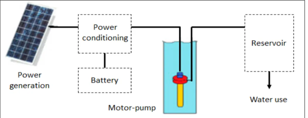
A PVPS is a system minimally composed of a photovoltaic (PV) array and a pump, converting the solar energy in mechanical energy in order to move water from one place to another. In a more advanced set up, the system can be completed by power electronics, or power conditioning unit, maximizing the quantity of energy used by the pump. These electronics are typically: Maximum Power Point Tracker (MPPT), a DC/DC or DC/AC converter. Moreover, the system often includes a way to store energy in the form of a battery or a water reservoir (i.e. chemically or mechanically). This energy storage allows to access water even when the solar resource is missing.
Figure 1.1: Block diagram of PVPS Adapted from Aliyu & al;, 2018
1.1.1 Photovoltaic array
PV array is the only power generator in a standard off-grid PVPS. Its role is to convert sun irradiance into electricity thanks to the photovoltaic effect inside semiconductor cells. This conversion results in the production of a DC current. Even though a current is produced, it can not be considered electronically as an ideal current generator because the internal structure of the cell interacts with the current generated, thus preventing a linear behavior. This property makes PV array output widely dependent on the load at the terminals and often justifies the need for power electronics. Typical maximum efficiencies of such arrays are about 15-20 %.
1.1.2 Motor pumps
The motor and the pump are often put together in a same device, but the analysis and understanding of the functioning of the whole are easier when they are investigated separately.
1.1.2.1 Electrical Motor
As photovoltaic pumping implies electricity as the energy source, only electrical motors are discussed here. In this case, the electrical motor is the part which converts electricity into mechanical movement, namely the rotation of a shaft, thanks to electromagnetic interactions between stator and rotor.
Numerous architectures exist for electrical motor, allowing it to take alternative current (AC) or direct current (DC), to vary the relation between torque, rotational speed, angular position, internal resistance, back electromotive force (e.m.f.), etc. Nearly all the technologies of electrical motors can be used for pumping water, but some are more common like the Permanent Magnet DC (PMDC) motor, which has the advantage of being compact and brushless, or the series wound DC motor, which has the advantage of having a high torque at the start of the motor (Beaty, 2006). Asynchronous AC motor are also used, because of their
low cost and long lifespan, but their efficiency and power density are markedly lower. Moreover, for some data availability reasons discussed further in 1.2.3.1, AC motor pumps are left out of the scope of this work.
1.1.2.2 Pump
The motor is then connected to a pump to transform the mechanical rotation power into pressure drop between the inlet and the outlet. Two main types of pump can be used in PVPS: the displacement pump (DP) and the centrifugal pump (CP).
a. Displacement pump
The displacement pump, or positive displacement pump, works by trapping a certain volume of water and by forcing it to move from the inlet to the outlet. In this type of pump, the flow rate Q is proportional to the rotational speed. This type of pump has the advantage that the flow rate is not much sensible to the head, making it particularly suitable for deep wells (N. Chandrasekaran, B. Ganeshprabu, & Dr. K. Thyagarajah, 2012).
b. Centrifugal pump
The mechanical load exerted by the fluids in centrifugal pumps is well adapted to PV power because the torque varies in the same way than the output flow rate. Therefore, when the input power is low, the pump can still work, lowering the rotational speed and thus pumping less water. This type of pump is more suitable for low-head application, with negligible friction head (Cheremisinoff & Cheremisinoff, 1989).
1.1.3 Power electronics
The power electronics deal with the conversion of the electricity produced by the PV arrays. It can change the type of current from DC to AC and vice-versa (respectively named inverter and
rectifier), or just convert a current from one voltage to another (converter). DC/DC converters used in PVPS usually work together with a MPPT, which allows to continuously get the maximum power output from the PV array. As AC motor pumps are not considered in the scope of this work, MPPT converter is the only power electronic system considered herein.
1.1.4 Energy storage
Here, the term energy storage is taken in a large sense and relates not only to battery storing electricity under chemical form, but also to reservoirs storing water at high elevations, allowing its use at any time of the day. An energy storage is not always necessary in a PVPS. Nevertheless, in some cases it can allow to use water when it is really needed, therefore resulting in a lower need.
As soon as an energy storage is considered, the notion of Load Losses Probability (LLP) can be used to evaluate the correct sizing of the energy storage. It represents the probability for the system to be unable to meet the demand and can be applied on systems with reservoirs in the same way than on systems with batteries (Hamidat & Benyoucef, 2009 ; Khatib & Elmenreich, 2016). The LLP is defined as the ratio between the lack of water and the total water volume required over a year.
1.2 Modeling of a PVPS
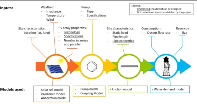
Understanding the outline of the global functioning of a PVPS is unfortunately not enough to ensure an efficient sizing. For correctly sizing a PVPS, it is first necessary to be able to predict correctly the output of the system. This section focuses on how the different components of the system are modeled in order to eventually constitute a complete PVPS model. For each step, the uncertainty coming from the data or the model are highlighted, if available. A summary of information needed, and models used in the modeling of a PVPS are described in Figure 1.2.
1.2.1 Fixed input data
1.2.1.1 Weather files
One of the main input data used for the simulation of a PV system is the weather file containing the irradiance data. For calculation time reasons, the weather files used cover no more than one year, and give different values such as temperatures, irradiance, and precipitation on an hourly basis. The way to summarize weather characteristics in a one-year file depends on the purpose of the weather file. For example, it can be constructed for representing a typical year - like TMY (Typical Meteorological Year), IWEC (International Weather for Energy Calculations) and CWEC (Canadian Weather for Energy Calculations) files - which thus reduces the presence of extreme conditions in the data (Wilcox & Marion, 2008). Therefore, this type of file should not be used in a case of worst-conditions sizing. Note that TMY files were developed by the NREL based on the algorithm created by Sandia National Laboratories, and this algorithm became a standard also used in IWEC and CWEC construction (CWEC, 2016 ;
Skeiker, 2007). On the opposite, special data can be built for representing extreme weather condition on one year, but these weather are not as common. (Nik & Arfvidsson, 2017)
Even before being processed in a one-year data, the data can be obtained by different means, yielding different biases in the final result. Three main families of data gathering strategies can be drawn: direct measurement, which are usually processed in Typical Year (TY) weather files; space interpolation, which uses the measurement files of the closest locations around to interpolate the weather of the considered place; and satellite observation, which relies on some indicators measured by meteorological satellites like the clearness index to infer the irradiance on the ground level (Al-Mofeez, Numan, Alshaibani, & Al-Maziad, 2012 ; Kumar & Umanand, 2005).
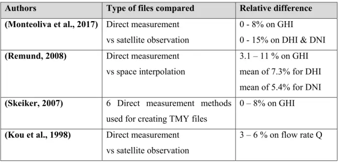
(Monteoliva, Villalba, & Pattini, 2017) studied three TY weather files coming from either satellites or ground stations measurements for the region of Mendoza in Argentina. They found that the mean yearly Global Horizontal Irradiance (GHI) could vary up to 8.3% between the data and could vary up to 15% in the case of Direct Normal Irradiance (DNI) and Diffuse Horizontal Irradiance (DHI) taken aside.
(Remund, 2008) processed the same analysis between data coming from ground measurements and from space interpolation given by the software Meteonorm. He found that the relative error on GHI values was comprised between 3.1% and 11%. For DHI and DNI, the mean relative errors were respectively 7.3% and 5.4%.
(Skeiker, 2007) ran a similar analysis by comparing TY weather files constructed from the same weather data records but with different algorithms. The researcher found that different algorithms could induce a relative difference between each other up to 8% for GHI data. Eventually it is stated that the algorithm inducing the smallest relative error is the one from Sandia National Laboratories.
(Kou, Klein, & Beckman, 1998) compared the throughput of a PVPS according to two hourly weather files, one coming from measured data (TY weather data) and the other generated from clearness index following a procedure proposed in the first edition of (Duffie & Beckman, 2013). It is found that the Root Mean Square Error (RMSE) in flow rate output between the two simulations ranges only from 3 to 6%. Nevertheless, this fairly good relative difference has to be considered with care because the authors used a pump model which was found to introduce important uncertainties as discussed in 1.2.3.1. In this same research work, the use of monthly averaged weather data is shown not to be suitable for PVPS simulation as it can widely underestimate the total volume pumped. Previously discussed results are gathered in Table 1.1.
Table 1.1: Relative difference in irradiance data in literature
Authors Type of files compared Relative difference
(Monteoliva et al., 2017) Direct measurement
vs satellite observation
0 - 8% on GHI
0 - 15% on DHI & DNI
(Remund, 2008) Direct measurement
vs space interpolation
3.1 – 11 % on GHI mean of 7.3% for DHI mean of 5.4% for DNI
(Skeiker, 2007) 6 Direct measurement methods
used for creating TMY files
0 – 8% on GHI
(Kou et al., 1998) Direct measurement vs satellite observation
3 – 6 % on flow rate Q
From the above it should be noted that weather files can bring significant errors, and therefore the choice of the weather file should be of prime interest in the modeling of a PVPS. In the following work, in order to reduce the relative error, only TY weather files based on the Sandia algorithm and relying on ground direct measurements are used (namely TMY, IWEC and CWEC files).
1.2.1.2 Site characteristics and consumption file
The site characteristics usually consist of the static head in the well, the horizontal distance between water source and reservoir, and the site location. As vertical head is a critical input for the PVPS output (Li, Jin, Akram, & Chen, 2017 ; Muhsen et al., 2017) and the water level is variable in a well through a year, it is often considered as the lowest water level of the well. In nearly all papers on PVPS modeling, the water demand is represented by an hourly file stating the output flow rate retrieved from the reservoir every hour. It is determined by the daily needs in water for a community or a farmer. This approach seems acceptable in the case where the water pumped is for domestic consumption which is about the same every day. However, such a daily profile may be oversimplified in the case of agriculture needs.
(Glasnovic & Margeta, 2007) paved the way for a new way to take into account variable consumption and variable water level into the well. In this work, focused on agriculture applications, the researchers considered the consumption as dependent on the weather, particularly on the rain fall, which reduces the need of water for the plants, and on the sun, which increases the need of water through evapotranspiration. In this study, the type of soil is also considered, influencing the soil moisture and the water infiltration, respectively linked to the water need and to the variable head in the well where the water is pumped. With this method the researchers are able to ensure that the phreatic table will not be depleted. They also find the counterintuitive outcome that the most critical months for sizing in Croatia are July and August, that is to say the months with the most important irradiance, resulting in higher evapotranspiration from crops.
1.2.2 PV generation modeling
The modeling of PV generation is a complex domain but has been already well investigated by researchers during the last three decades. Nowadays, some models are widely used and have been implemented in some ready-to-use tools like the Python package pvlib-python (Holmgren, Hansen, & Mikofski, 2018). This package provides classes and functions
simplifying the use of many models applying to solar cell, irradiance, absorption, module temperature and others. As the PV generation modeling is not the core of this work, the coming section is aimed at giving an overview of the possibilities included in pvlib-python. This overview focuses only on the models that were considered as the most commonly used in literature, and that are used by default in the results found in CHAPTER 3
1.2.2.1 Irradiance models
Classic irradiance data gives the irradiance on a horizontal plane: these are usually named diffuse horizontal irradiance (DHI) and global horizontal irradiance (GHI). To get the actual irradiance on a tilted plane, an irradiance model is then needed. The irradiance models proposed in pvlib-python are the following: isotropic, Klucher, Hay-Davies, Reindl, King and Perez. Detailed explanations for each model can be found in (Duffie & Beckman, 2013).
The isotropic model is the default one in pvlib-python and is widely used in related literature, mostly because it is easy to use with formulas that can be calculated by hand. It assumes that the direct normal irradiance (DNI) comes from the point where the sun is in the sky and then the DHI is spread evenly, in a isotropic way, through the rest of the sky. (Loutzenhiser et al., 2007) found that the isotropic model had a relative error of 14% between predicted and measured irradiance on a vertical surface. Then, the more the surface tilt approaches the horizontal position, the less the relative error is. In the same paper, it is also stated that Perez model seems to be the best, with a maximum of 9% relative error. Nevertheless, as the isotropic model is still more commonly used in the literature reviewed, it is kept as the default irradiance model in order to ease the comparison with previous works.
1.2.2.2 Absorption models
Irradiance models allows to evaluate the incident irradiance on the array, but then two coefficients are needed to get what is called the effective irradiance, that is to say the irradiance practically available for the solar cell to convert.
The first coefficient is the incidence angle modifier (IAM). It can be obtained by 5 different models in pvlib-python: ASHRAE, physical, Martin-Ruiz, interpolation, SAPM. The default IAM model is the physical model, also described in (De Soto, Klein, & Beckman, 2006), and relying on some very common physical equations for the transmission of light like the Fresnel Laws. The second coefficient is the spectral modifier. This spectral modifier comes from the difference in the spectral profile of light depending on the quantity of air and water vapor the light has to go through before arriving on the PV cell. This modifier is empirical and is found from databases giving coefficients for each cell material available depending on air mass and air humidity.
(De Soto et al., 2006) state that IAM and spectral modifier are significant only for incidence angles superior to 70° and 80° respectively. At these angles, it is unlikely that a PVPS would still pump water, so these absorption models might not be of special concern.
1.2.2.3 Cell temperature models
The cell temperature model is used in pvlib-python to determine the temperature of the solar cells as a function of incident irradiance, air temperature, wind speed, materials of the module and mounting (open rack, roof-top, insulated-back). Three models are proposed: SAPM, PVSyst, and Faiman. The model used by default is the PVSyst model (PVsyst, s.d.) which considers default values for the silicon, and retrieves the required data from the module parameters contained in CEC or Sandia Module Database.
1.2.2.4 Solar cell models
Three solar cell models are implemented in pvlib-python: the empirical model developed by the Sandia National Laboratories (King, Kratochvil, & Boyson, 2004), the theoretical five parameters single-diode model (SDM) of (De Soto et al., 2006) and the six parameters SDM
derived from De Soto’s work and developed at the California Energy Commission (CEC) (Dobos, 2012).
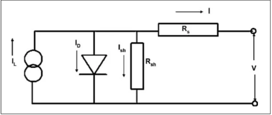
The most common model is the five parameters SDM developed by (De Soto et al., 2006). As it is directly used by the direct coupling model in order to find the operating point between PV array and motor pump, this model deserves a focus. It represents a PV cell as an electrical circuit composed of one direct current generator producing a photocurrent IL, one diode
subjected to a current ID with a saturation current I0 and an ideality factor parameter a, and two
resistances, one in parallel RSH and one in series RS. The equivalent circuit is in Figure 1.3 and
the corresponding equation giving the current in the load at the terminals of the cell is equation 1.1. 𝐼 𝐼 𝐼 𝑒𝑥𝑝𝑉 𝐼𝑅 𝑎 1 𝑉 𝐼𝑅 𝑅 (1.1) With 𝑉 𝐼 ∗ 𝑅 (1.2)
This model has been popularized since De Soto & al showed the five unknown parameters previously mentioned can be easily found from typical manufacturer’s datasheets. The manufacturers minimum input data needed are ISC, VOC, Impp, Vmpp and αSC, usually given at
STC conditions. It is then processed in a system of five nonlinear equation, all coming from boundary conditions on equation 1.1, with five variables unknown, and returns the values of
Figure 1.3: Electrical equivalent circuit of SDM Taken from De Soto (2006)
IL,ref, I0,ref, RS,ref, RSH,ref, and aref. Later (Shannan, Yahaya, & Singh, 2013) measured the relative
error between measured and predicted output power of the De Soto SDM and found that it was inferior to 1% for cell temperature between 0°C and 50°C.
1.2.2.5 PV module database
The PV module database is not a model but is another important feature of pvlib-python. Indeed, the package can access two databases of PV modules: the CEC modules database and the Sandia Modules database. The CEC modules database comes from NREL’s System Advisor Model (SAM) (Blair et al., 2014) and is the one used in this work. It is updated on a regular basis and provides many details and specifications on the PV modules, like the maximum power in STC, the six parameters of Dobos’s SDM (can be directly used by De Soto’s SDM as well), cell material, size of the module, number of cells, etc. As of January 2020, more than 21000 PV modules are indexed in this database.
1.2.3 Motor pump modeling
The motor pump modeling is one of the two key parts of PVPS modeling, along with PV generation modeling. However, contrary to the PV generation case, the existing literature does not agree on the models to use for modeling pumps, and different papers use different approaches on that topic. The following section synthetizes the two main approaches: empirical and theoretical, and describes the corresponding models found in the literature. Motor pump models are more thoroughly described than previous PV models because their implementation represents an important part of the originality of the developed software. In the following work and in part of the literature, motor and pump are considered as a whole, mounted in a same machine, and therefore the terms motor pump and pump can be used interchangeably.
1.2.3.1 General strategy
Electrical motor pump modeling is a vast subject as many different technologies of motors exist, relying on different electrical principles and assemblies. Moreover, the data provided by pump manufacturers can differ widely, preventing the researchers from constructing a simple and practical model for motor output prediction. The purpose of modeling the motor-pump group is to link the input electrical power to the water discharge. To his end, two equations are needed:
• The first equation is the I-V relation of the motor:
𝐼 = 𝑓1 𝑉, 𝑇𝐷𝐻 (1.3)
Indeed, as the main resistance to the shaft rotation is the behaviour of the liquid in the pump casing, and as the speed of the rotor influences the electromagnetic field of the electrical circuit, the total dynamic head (TDH) is a major variable in the electrical function f1. Equation f1 is used in cases of direct-coupling between PV array and pump, in order to find the operating point by comparing the I-V relations of the PV array and of the pump.
• The second equation is the discharge-power relation of the motor:
𝑄 = 𝑓2 𝑃, 𝑇𝐷𝐻 (1.4)
Where Q is the output flowrate of the pump in m3/h or L/min.
In equations 1.3 and 1.4, the current I, the voltage V and the power P can be replaced by each other as they are constantly linked by:
𝑃 = 𝐼 ∗ 𝑉 (1.5)
In most cases the pumps are designed to be connected to an ideal voltage source, that is to say a source with constant voltage and from which infinite power can be drawn. For common pumps connected to the grid this assumption is correct as the range of use is often way below
the limits of the grid. In this case, the first function f1 is simplified in I = f1, V=k (TDH). And as
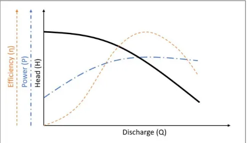
P and I can be replaced by each other, P is function of TDH, and the output flow rate becomes only dependent on TDH: Q = f2 (TDH). These simplifications result in the common specifications for pumps as illustrated in Figure 1.4. Here, function f2alone is enough for predicting the pump output, and the information on the power P is given on an indicative basis to forecast the energy cost of the pump. The efficiency curve can be found from these two, and therefore is not of prime importance.
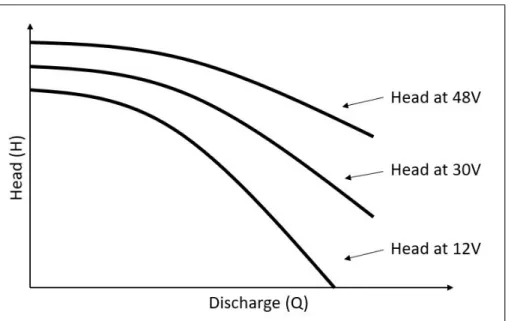
In the case of a pump connected to a finite power source, like a PV array, the operation of the motor pump is different. It depends on V and I, and none of the function f1 of f2 can be simplified. Therefore, specifications need to be given at different voltage, resulting in more complete specifications as shown in Figure 1.5. Similar curves must be provided for power.
Figure 1.4: Standard characteristics given for an electric motor pump
As AC motor pumps are often designed to be connected to the AC grid, they typically include restricted specifications at only one given voltage. On the opposite DC motor pump are mainly designed to work on batteries or PV arrays, so specifications are given for multiple voltages. This work focuses on DC motor pumps because it is the only category for which manufacturers provide sufficient data in order to build a model with a finite and variable power source. AC motor pumps could be investigated in future work.
1.2.3.2 Empirical approaches
These approaches consist in fitting curves for the existing pump data, and then to use these curves to interpolate and extrapolate extra points. Therefore, the pump data must be complete enough to ensure a correct curve fitting. This complete data can be given by the manufacturer of the pump or can be obtained by some tests run on the pump prior to the modeling or sizing. As the manufacturer rarely give enough data, except some companies like (SunPumps, s.d.), the researchers have to carry out tests on the pump before the study in most cases (Hadj Arab,
Figure 1.5: Specifications needed for PV array connection
Benghanem, & Chenlo, 2006 ; Hamidat & Benyoucef, 2008 ; Jafar, 2000). Once the pump data is complete enough, the following approaches can be applied.
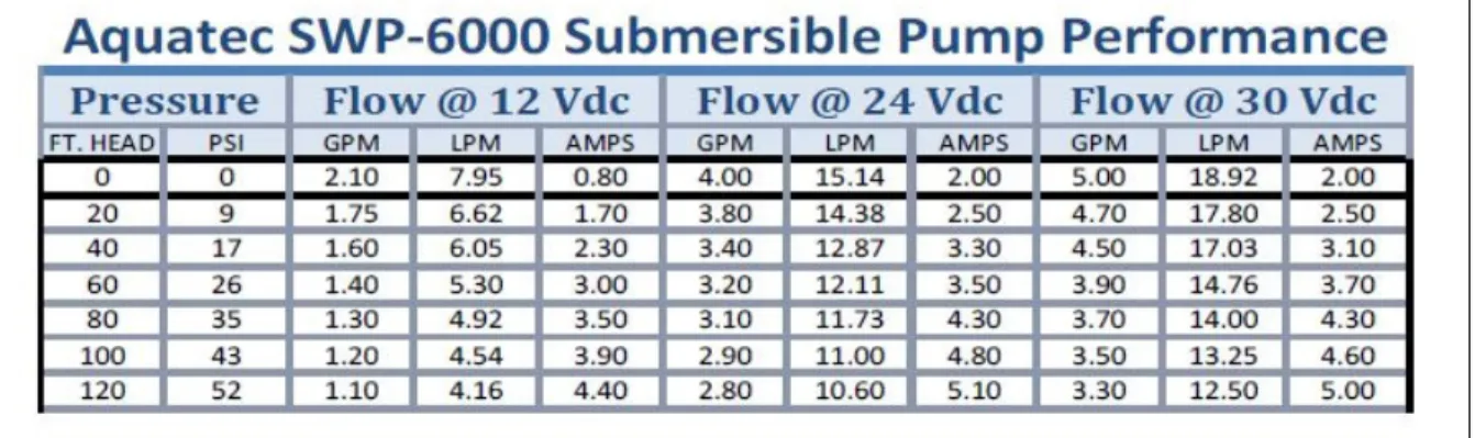
A typical pump datasheet can be found in Figure 1.6. It contains the flow rate Q and the current I drawn for different voltage and for different head. In total, it gives a certain amount of points (TDH, V, I, Q) that can be used later. In Figure 1.6, three voltages and seven heads are given, resulting in 21 points (TDH, V, I, Q).
a. Kou’s model
(Kou et al., 1998) determine the function V=f1 (I, TDH) and Q=f2 (V, TDH) from manufacturer’s data. To obtain these two functions, they fit the data with a 3rd order polynomial with cross terms. The resulting multivariate polynomial functions f1 and f2 have the form of equation 1.6.
𝑧 = 𝑧 𝑎 ∗ 𝑥 𝑎 ∗ 𝑥 𝑎 ∗ 𝑥 𝑏 ∗ 𝑦 𝑏 ∗ 𝑦 𝑏 ∗ 𝑦 𝑐 ∗ 𝑥 ∗ 𝑦 𝑐 ∗ 𝑥 ∗ 𝑦 𝑐 ∗ 𝑥 ∗ 𝑦 𝑐 ∗ 𝑥 ∗ 𝑦
(1.6)
As the functions f1 and f2 are third order polynomials on I and TDH, it means that the pump data needs to provide information for at least four different voltages and heads, and needs to have a total of at least 16 points (TDH, I, V, Q) in order to yield a correct curve fit.
Figure 1.6: Typical DC pump datasheet Taken from www.aquatec.com
Jahnig (Jahnig D., Klein S.A., & Beckman W.A., 1998) investigated this model for validation. He found a significant discrepancy between expected flow rates and measured flow rates. The relative error is around 20-40% for high irradiance and could even be infinite for irradiance levels below 550W/m2. The authors explain the difference by incorrect data given by the pump manufacturer, but the author did not investigate the model with corrected pump data, so it is not possible to decorrelate the error from the model and the error from the incorrect pump data. It is also stated that at least 10% of the discrepancy comes from the four parameters single-diode model used for PV prediction. As this single-single-diode model is now outdated, some improvements could be expected with Kou & al.’s model.
The same model is used later by (Martiré, Glaize, Joubert, & Rouvière, 2008) for modeling f2 only. In their paper, the authors fit an affinity law in order to get an algebraic equation more convenient to use. Equation f1 is useless in this case as the electric power is processed through a MPPT. Indeed, it is considered that the electric power is always maximised. The resulting relative errors between predicted and measured flow rates are about 15% in the morning, and stabilize around 5% during the day, at the time the pump operates in steady state.
b. Hadj Arab’s model
Hadj Arab (Hadj Arab et al., 2006) and Djoudi Gherbi (Djoudi Gherbi, Hadj Arab, & Salhi, 2017) propose another empirical model for modeling the pumps. Even though their research relies on data obtained by tests made on the pump in their laboratory, it can also be used on manufacturer’s data if the data set is complete enough. This model proposes to use a linear equation for I-V curve of pump, corresponding to f1:
𝐼 = 𝑎 + 𝑏 ∗ 𝑉 (1.7)
The flow rate Q is dependent on voltage V through a quadratic equation, corresponding to f2:
Eventually, all coefficients a, b, c, d, e are dependent on TDH following either a quadratic (Hadj Arab et al., 2006) or cubic equation (Djoudi Gherbi et al., 2017):
𝑎 = 𝑎 + 𝑎 ∗ 𝑇𝐷𝐻 + 𝑎 ∗ 𝑇𝐷𝐻 + 𝑎 ∗ 𝑇𝐷𝐻 𝑏 = 𝑏 + 𝑏 ∗ 𝑇𝐷𝐻 + 𝑏 ∗ 𝑇𝐷𝐻 + 𝑏 ∗ 𝑇𝐷𝐻 𝑐 = 𝑐 + 𝑐 ∗ 𝑇𝐷𝐻 + 𝑐 ∗ 𝑇𝐷𝐻 + 𝑐 ∗ 𝑇𝐷𝐻 𝑑 = 𝑑 + 𝑑 ∗ 𝑇𝐷𝐻 + 𝑑 ∗ 𝑇𝐷𝐻 + 𝑑 ∗ 𝑇𝐷𝐻 𝑒 = 𝑒 + 𝑒 ∗ 𝑇𝐷𝐻 + 𝑒 ∗ 𝑇𝐷𝐻 + 𝑒 ∗ 𝑇𝐷𝐻 (1.9)
In order to apply the model to a pump, the data requires at least three voltages and four different heads, for a total of at least 12 points (TDH, P, Q) and 8 points (TDH, I, V), or 12 points (TDH, I, V, Q). The model has been tested by the researchers on two centrifugal and two positive displacement pumps. When considering a quadratic equation for the variation of the coefficients with head, the relative error between model and measures remains below 14% for all heads on centrifugal pumps, and below 5% for positive displacement ones. When the input data of the model is reduced to the minimum of nine points, the model still manages to fit the measurements, adding only a maximum of 5% to the relative error. When considering a cubic equation for the variation of the coefficients, the relative error diminishes below 10% for all heads on centrifugal pumps and remains below 4% for positive displacement pumps. In this case the input data needs to be complete, as a higher order of polynomial regression obviously requires more data points for the fitting.
c. Hamidat’s model
Hamidat A. proposed another model for modeling a pump coupled to a PV array through a MPPT (Hamidat & Benyoucef, 2008). The study only considers a MPPT setting, therefore, as mentioned earlier, f1 is not needed. The equation for f2 is still required and is given by equation 1.10.
This equation links the electric power P with a polynomial function taking the flow rate Q as the relevant variable. This form is however not convenient for determining the output flow rate according to the power produced by the PV array. Authors thus decide to use Newton-Raphson’s root finding method to get Q from P. The coefficients of the polynomial are dependent on the TDH following a cubic equation such as in equation 1.9, therefore minimum pump data in this case include four different heads, and 16 points (TDH, P, Q).
Their model is then used to run simulations for four locations with two different motor pumps with different head but is not compared with actual measurements. The relative error cannot be assessed then. This model is also used in (Gualteros Martinez, 2017) but without assessment of the model validity either.
1.2.3.3 Theoretical approach on DC motor pumps
The prediction of the output of motor pump can also be carried-out by analysing the electrical architecture of the motor used. This approach is used by (Khatib & Elmenreich, 2016) and is briefly discussed in the following section.
DC motors can be modelled electrically as a resistance, an inductance and a voltage generator put in series (N. Chandrasekaran et al., 2012 ; Tantos, 2011b). This voltage source is surrounded by a magnetic field Φ which is produced from permanent magnet or from electromagnets fed in electricity by the system. In the latter case, the magnetic field is produced by an inductance Lf, whose internal intensity If and voltage Vf can be dependent or not on Va
In this model the resistance Ra and inductance La are intrinsic properties of the motor armature,
Ra accounts for the wire resistance and the brushes resistance. Stationary operation is assumed
and as the motor is run by DC current, it is possible to put aside the transitional effects and not to consider La nor the inertia of the mechanical load.
The voltage in the armature is:
𝑉 = 𝐼 ∗ 𝑅 + 𝐸 (1.11)
The reverse voltage Eg is induced by back electromagnetic force (e.m.f.) and is proportional to
the angular speed of the shaft and to the magnetic flux:
𝐸 = 𝐾 ∗ 𝛷 ∗ 𝜔 (1.12)
The motor torque Tm is linked to the armature through:
𝑇 = 𝐾 ∗ 𝛷 ∗ 𝐼 (1.13)
Then the output pump torque Tp is often said to be proportional to the squared rotational speed
of the shaft.
𝑇 = 𝐾 ∗ 𝜔 ↔ 𝑇 ∗ 𝜔 = 𝑃 = 𝐾 ∗ 𝜔 (1.14) Figure 1.7: Electrical model of a DC motor-pump
However, it has to be noticed that this proportional relation is an affinity law, therefore assuming that the efficiency, included in K, is constant with ω. (Martiré et al., 2008) state that this approximation is correct on relatively small motors, but underline the fact that the efficiency is dependent on the flow rate, and as the flow rate is dependent on the head and the rotational speed, it is equivalent to say that the constant K must be dependent on TDH. Hence:
𝑇 = 𝐾 (𝑇𝐷𝐻) ∗ 𝜔 (1.15)
As a result,
𝑉 = 𝑅 ∗ 𝐼 + 𝐾 ∗ 𝐾
𝐾 (𝑇𝐷𝐻)∗ 𝛷 ∗ 𝐼
(1.16)
Equation 1.16 gives a direct relationship between the voltage and the current, which is the first function wanted f1. Second equation f2 comes from the conservation of energy between electrical and mechanical power (Khatib & Elmenreich, 2016).
𝑄 ∗ 𝛥𝑝 = 𝑃 = 𝜂 ∗ 𝑃 ↔
𝑄 = 𝜂 (𝑄) ∗ 𝑃
𝑔 ∗ 𝜌 ∗ 𝑇𝐷𝐻
(1.17)
Where Δp is the pressure difference between input and output of pump in Pa.
𝜂 (𝑄) can be fitted with polynomial, as in (Martiré et al., 2008), found from 𝜂 (𝑃 , 𝑇𝐷𝐻) in MPPT coupling cases, or from 𝜂 (𝐼, 𝑉, 𝑇𝐷𝐻) in direct coupling cases. If not enough data is given, it can be considered as constant, even though it adds substantial uncertainty on the output.
The values of Kp and Km can be found sometimes in manufacturer datasheets. If not available,
they can be computed from the specifications given or by running some tests on the pump (Tantos, 2011a). The method described by Tantos consists in using four particular operating points: no-load, stall, maximum efficiency and maximum output power. These points are
typically given at rated voltages and in stationary conditions. But sometimes pump manufacturers do not give these points and modeling the motor cannot be done with the theoretical approach of Tantos. (Kolhe, Joshi, & Kothari, 2004) use a similar approach for the motor but considers a more advanced model for the centrifugal load, taking into account the moment of inertia and the viscous torque constant of the pump, resulting in a different form for f2. Even so these data are very rare in manufacturer datasheet, therefore it has been decided not to include the Kolhe model in the scope of this work. According to the figure 11 in (Kolhe et al., 2004), the relative error on overall efficiency between prediction and measurements ranges from 27% at 300W/m2 to 7% at 700W/m2.
Above theoretical approach can be used to model different types of motor. In the scope of this work, one is particularly investigated because it is more widely described in the literature reviewed: the permanent magnet DC motor. In the case of such a motor, the magnetic field Φ is constant in any conditions, which simplifies further the equations. Equation f1 becomes:
𝑉 = 𝑅 ∗ 𝐼 + 𝐾 ∗ 𝐾
𝐾 (𝑇𝐷𝐻)∗ 𝐼 ↔
𝑉 = 𝛼 ∗ 𝐼 + 𝛽(𝑇𝐷𝐻) ∗ 𝐼
(1.18)
Equation f2 can be used normally afterward (equation 1.17). This model has the advantage of requiring less information on pumps. First, it needs the electrical architecture of the motor, and then in the merest case where Kp is considered as constant with TDH, only 2 (I, V) points and
1 (Q, P, TDH) point are needed, or only 1 (Q, P, TDH) point if coupled with a MPPT.
1.2.3.4 Operating range of the pump
In the previous papers, researchers always assume that the motor pump works in stationary operation. However, to improve the accuracy of the empirical and theoretical approach, transitional effects should be taken into account. These transitional effects happen typically in
the morning at the start of the motor, and more generally for high variations in irradiance during the day, for example in the case of variable partly cloudy conditions. Most studies on PVPS modeling consider a very sunny weather, with very smooth irradiance variations through the day, avoiding the researchers to address these transitional effects. It can be noticed that (Martiré et al., 2008) report their largest relative errors between prediction and measurement in the morning, right after the pump begins to operate.
Being able to model unsteady operations would allow to better predict the exact moment when the pump starts and when it stops. To consider this, more information is needed: the starting voltage and current, and the maximum power acceptable. These characteristics can originate from the motor pump itself or from the integrated controller, if existing.
Nevertheless it is unlikely that pump manufacturer datasheets give such characteristics, and other strategies must be used. The most evident is the prior testing of the pump to gather the required information, but such strategy requires to have access to a test bench.
The second strategy is to analyse the motor with a theoretical approach. (Singer & Appelbaum, 1993) investigated the starting characteristics of a DC motor with this approach, and find that the starting current Ist could be linked to the rated current Irated for the four main electrical
architectures of DC motor. For example, for PMDC motor it is found that Ist = 1.2 * Irated.
Thanks to this work, the consideration of the range of functioning and the starting characteristics could be made simpler, and could be implemented in a model as soon as the pump electrical architecture is known.
1.2.3.5 Summary table
The following table summarizes the previously discussed pump models and their relative accuracy. Relative errors are related to the output flowrate values, unless specified otherwise.
Table 1.2: Summary of pump models
Name and papers Relative error
Minimum Data size required
Coupling method applicability
Kou model
(Kou et al., 1998) and (Jahnig D. et al., 1998)
20 – 40% 16 (TDH, I, V, Q) points + 4 different V
+ 4 different TDH
Direct / MPPT
Hadj Arab model (Hadj Arab et al., 2006)
< 5% for DP < 14% for CP 9 (TDH, I, V, Q) points + 3 different V + 3 different TDH Direct / MPPT
Hadj Arab model
(Djoudi Gherbi et al., 2017)
< 4% for DP < 10% for CP 12 (TDH, I, V, Q) points + 3 different V + 4 different TDH Direct / MPPT Hamidat
(Hamidat & Benyoucef, 2008)
Not Assessed 16 (TDH, P, Q) points + 4 different V + 4 different TDH
MPPT
Theoretical
(Mokeddem, Midoun, Kadri, Hiadsi, & Raja, 2011)
Not Assessed 2 (TDH, I, V) points + 1 (TDH, P, Q) point + Electrical architecture
Direct / MPPT *
Theoretical model for f1
(Kolhe et al., 2004) 7 – 27% on motor-pump efficiency 2 (TDH, I, V) points + 1 (TDH, P, Q) point + Electrical architecture Direct / MPPT *
Theoretical model for f2
(Martiré et al., 2008)
5 – 15% 6 (TDH, P, Q)
+ 6 different Q at a given TDH
MPPT * Starting characteristic consideration possible without additional data
1.2.4 Hydraulic circuit
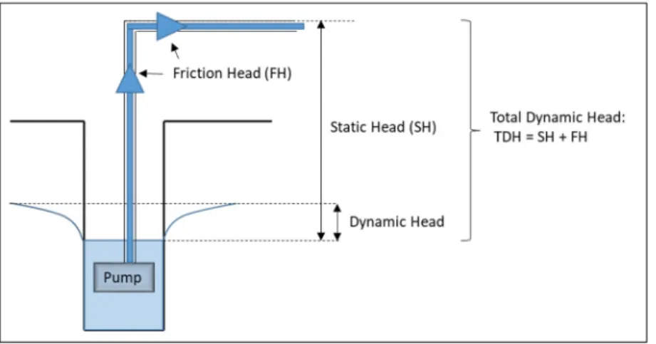
The terminology used to refer to the different heads in a hydraulic circuit is not standardized among all papers. In this work, the following terminology is used: friction head (FH) refers to the head caused by the friction in the pipes, dynamic head (DH) refers to the variable level of water at the water source, static head (SH) refers to the total vertical head in the system, thus including the dynamic head, and total dynamic head (TDH) is the maximum global head seen by the pump. The different head are summarized in Figure 1.8.
Except (Glasnovic & Margeta, 2007) and (Campana, Li, & Yan, 2013), all researchers working on PVPS consider static head as constant in time, with no dynamic head. The main reason for this is that the dynamic head is difficult to predict and depends on complex geological systems, often out of the field of the researchers in PVPS, who are mainly specialized in mechanics and electronics. However, it has to be noticed that it may be a major omission in the modeling of a pumping system as discussed in 1.2.1.2.
Concerning the computation of friction head, this field of fluid mechanics is well developed, and some models are very commonly applied. For example, the Darcy–Weisbach equation (Douglas, 2005) is often used in PVPS modeling along with the fluid and pipes properties to evaluate the head due to friction effects in the pipes (Khatib & Elmenreich, 2016 ; Mokeddem et al., 2011). The Darcy-Weisbach equation needs a friction factor which has to come from other relations dependant on the regime of the fluid in the pipe. Hagen-Poiseuille and Colebrook equations can be used respectively for laminar and turbulent flows with a not significant relative error (Bell, s.d.) for a PVPS case.
These fluid models are already implemented by researchers in different packages available online. Notably, the open-source project fluids (Bell, s.d.) proposes a ready-to-use package
written in Python and implementing many fluid models and standard pipes and fluids properties.
1.2.5 Global modeling procedure
After having detailed the modeling of the different part of the system, a last focus should be put on how to link all these models to eventually reach the prediction of output water flow rate. Two cases can be drawn: the modeling with a MPPT converter between PV array and pump, or the modeling without it.
1.2.5.1 MPPT coupled modeling
Using a MPPT is the easiest coupling method to model, and the most widely used because it can bring significantly better water output for the PVPS (Aliyu et al., 2018 ; Muhsen et al., 2017). It consists in simply considering the total power produced by the PV array, with no consideration of current and voltage, and to use it as input power for the pump. The power can be reduced by a given percentage to take into account the losses in the conversion. This MPPT coupling is used in (Gualteros Martinez, 2017 ; Hamidat & Benyoucef, 2008 ; Meunier et al., 2019).
1.2.5.2 Direct-coupling modeling
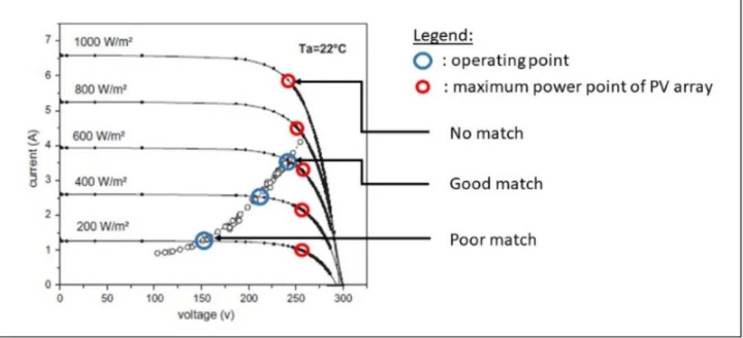
The direct coupling method is for systems including no power electronics between PV array and the pump. This type of system can be preferred in order to simplify the set-up in the perspective of having a more reliable PVPS in time or to lower the cost. Such systems often use PMDC motor pumps for load-matching and reliability reasons (Djoudi Gherbi et al., 2017 ; Kolhe et al., 2004 ; Mokeddem et al., 2011). In this case the I-V operating point between PV array and the pump must be found. It can be defined as the intersection between the I-V curve of the PV array and the I-V curve of the pump (represented by the function f1 described in 1.2.3.1.) as shown in the Figure 1.9. This figure shows the issue of load-matching: the PV array
and pump I-V curves can sometimes not intersect or can intersect far from the maximum power point of the PV array. In this case the power produced by the PV array is not maximised and it results in a low output from the PVPS.
In terms of costs and output flow rates, no global comparison between direct and MPPT coupled systems was found in the literature. It can be noticed that (Mokeddem et al., 2011) reported pump efficiencies up to 25% on a PMDC pump directly coupled, whereas (Hamidat & Benyoucef, 2008) stated that efficiencies up to 40% are reachable for the same type of pumps, suggesting that direct systems cannot be as efficient as MPPT systems. However this is highly dependent on the match quality between pump and PV array, therefore this difference in efficiency cannot be generalized in any way. The following research tries to address this question by running comparisons on a big set of pump and locations.
1.2.5.3 Friction head and total head computation
If the water level is considered as fixed, as discussed in 1.2.4, a static head can be selected for each location, and only the friction head coming from pipes friction and fittings has to be added to obtain the TDH. In most cases, if the pipes are correctly sized, the TDH should not vary widely over the constant SH. Therefore, for each pumping system, a simplified function
Figure 1.9: Operating point in direct-coupled systems. Adapted from Mokeddem & al.
I = f1,TDH=k (V) can be found. This simplified function is implicitly assumed in the work of
(Hadj Arab et al., 2006) and (Hamidat & Benyoucef, 2008).
If this approximation cannot be done, TDH should be computed from discharge Q with a function TDH = f3 (Q). Then it is possible to iterate on f1, f2 and f3 until converging to the TDH researched, or to try to integrate f3 into f2 so as to avoid the necessity of looping until convergence (Meunier et al., 2019).
1.2.5.4 Global relative error
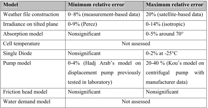
The following table summarizes the different relative errors that correspond to each model previously discussed and used through the whole simulation of a PVPS.
Table 1.3: Summary of minimum and maximum of typical relative errors for models used in PVPS modeling
Model Minimum relative error Maximum relative error
Weather file construction 0–8% (measurement-based data) 20% (satellite-based data) Irradiance on tilted plane 0-9% (Perez) 0-14% (isotropic)
Absorption model Nonsignificant 0-5% around 70°
Cell temperature Not assessed
Single Diode Nonsignificant 0-2% at -25°C
Pump model 0-4% (Hadj Arab’s model on
displacement pump previously tested in laboratory)
20-40 % (Kou’s model on centrifugal pump with manufacturer data)
Friction head model Nonsignificant Nonsignificant
Water demand model Not assessed
It can be noticed that the expected relative errors of each model depend on the situation in which the model is used. It is particularly true for pump modeling, where few papers present relative error assessment, and even when given, it is strongly linked with the other factors of
the study (data size of pump specifications, sunny location, electrical architecture, etc.). Therefore, a special focus should be put on evaluating the performance of each pump model on a same experimental set-up.
1.3 Sizing procedures
As detailed in 1.2 the prediction of a PVPS output still needs investigations to determine what is the best way to make an accurate prediction, in particular which pump model to use to this end. Still, some researchers worked in parallel on the sizing of such systems.
As represented in Figure 1.10, sizing is basically the reverse process of modeling. The output of the modeling, water flow rate in this case, becomes the input of the sizing; and the inputs like PV array and pump become the expected output. Therefore, the sizing process uses the same models than the modeling process to be able to choose the best elements during the sizing. This highlights the need of an accurate modeling to ensure a correct sizing.
The standard fixed inputs for the sizing are the water consumption, the weather files and the site characteristics. Then the variables to size of a PVPS are numerous, and the sizing should ideally be made on any of these variables, like PV array size, tilt, PV module, coupling method, motor-pump, reservoir size… But all these variables interact between each other, resulting in huge complexity. To simplify the problem, it has to be assumed some values, and therefore to focus the sizing on a few variables only. The sizing methods can be gathered in two groups: the intuitive and numerical methods. The intuitive method allows to size a good number of variables but always with neglecting a lot of interaction between the elements of the system, resulting in a poor output prediction, whereas numerical methods often restrict the number of variables to size but use a more reliable analysis based on whole iterative simulations. The global structure of the methods is described in Figure 1.10, and each of them are explained further in the next sections.
1.3.1 Intuitive methods
Intuitive method refers to any sizing method where each component and variable is selected following some simple principles linking the different specifications and components to each other. The research using these methods often consider the worst month, which is not necessarily easy to find as detailed in 1.2.1.2, or monthly average data. The Life Cycle Cost (LCC) can be used in these methods to find the more cost-efficient option. LCC is the cost of the system including the initial investment, the operational costs during its whole lifespan and the end of life value. The LCC can be computed using different method, including more or less details in the assessment of the different costs, but it is often considered as the same than the Net Present Value (NPV) of the project, thus including the discounted cash flows through time.
(Campana et al., 2013) used an intuitive method to size a whole system. They start by assessing the water need with a dynamical model, and then adapt an intuitive method for the selection of the other components. Basically, the components are arbitrarily chosen as long as they match the needed load. They use a factorial experimental design to evaluate the best configuration