Truchon: CIRPÉE and Département d’économique, Université Laval
Gordon: Corresponding author. CIRPÉE and Département d’économique, Université Laval
We thank Mohamed Drissi-Bakhkhat for his detailed comments on a previous version.
Cahier de recherche/Working Paper 06-25
Statistical Comparison of Aggregation Rules for Votes
Michel Truchon Stephen Gordon
Avril/April 2007
Abstract:
If individual voters observe the true ranking on a set of alternatives with error, then the social choice problem, that is, the problem of aggregating their observations, is one of statistical inference. This study develops a statistical methodology that can be used to evaluate the properties of a given voting or aggregation rule. These techniques are then applied to some well-know rules.
Keywords: vote aggregation, ranking rules, figure skating, maximum likelihood,
optimal inference, Monte Carlo, Kemeny, Borda
Contents
1 Introduction 1
1.1 The social choice problem . . . 1
1.2 A Monte Carlo approach . . . 2
1.3 Summary of the results . . . 2
1.4 Contents . . . 3
2 Methodology 3 2.1 Vote aggregation: notation and definitions . . . 3
2.2 Statistical models of voter choice . . . 4
2.3 Criteria for evaluating aggregation rules . . . 6
2.4 Summary of the problem . . . 6
3 Modelling choices 7 3.1 Statistical model . . . 7
3.2 Aggregation rules . . . 7
3.2.1 The Borda rule . . . 8
3.2.2 The Kemeny Rule . . . 9
3.2.3 The Maximum Likelihood rule . . . 10
3.2.4 The ISU-94 Rule . . . 12
3.2.5 The ISU-98 Rule . . . 13
3.3 Loss functions . . . 15
3.4 Simulation methodology . . . 15
4 The results in brief 18 5 Conclusion 20 Appendices 24 A Finding Kemeny orders and choosing among them 24 B Description of the results 25 B.1 Simulations with three judges and (α, β) = (1.1, 0.9) . . . 25
B.2 Simulations with nine judges and (α, β) = (1.1, 0.9) . . . 27
B.3 Simulations with nine judges and (α, β) = (1.0, 0.3) . . . 29
B.4 Simulations with nine judges and a constant probability . . . 31
B.5 Simulations with nine judges and (α, β) = (0.4, 1) . . . 33
List of Tables
1 Distribution function parameters and choice probabilities . . . 7
2 Illustration of the ISU-94 rule . . . 13
3 Illustration of the ISU-98 rule . . . 14
4 Loss function parameters and implications for costs of errors . . . 16
5 Description of the simulations . . . 18
6 Relation between different rules in terms of expected loss with 3 judges and η = 1 . . . 26
7 Probabilities and empirical frequencies of cycles with α = 1.1, β = 0.9 . . . . 27
8 Relation between different rules in terms of expected loss, α = 1.1, β = 0.9, η = 1 . . . 28
9 Probabilities and empirical frequencies of cycles with α = 1, β = 0.3 . . . 29
10 Relation between different rules in terms of expected loss, α = 1, β = 0.3, η 6= 2 . . . 30
11 Relation between different rules in terms of expected loss, α = 1, β = 0.3, η = 2 . . . 30
1
Introduction
1.1
The social choice problem
The question of how best to aggregate individual preferences or rankings is one of the oldest and best-known in the social sciences. Many organization must rank candidates for a posi-tion, a scholarship or a prize on the basis of rankings or preferences expressed by a panel of voters, judges or experts. Other organizations seek to rank investment projects on the basis of multiple criteria such as short term and long term profitability, social impact, environ-mental impact, and so on. In some democratic bodies or societies, the goal is the aggregation of individual preferences, expressed as orders or pre-orders, into a collective preference. In judged sports such as figure skating, diving, synchronized swimming and gymnastics, the task is the aggregation of individual assessments of the performance by a panel of judges into a final ranking.
All the above problems are formally the same. There is a set of candidates or alternatives to be ranked, a set of voters, judges or experts who are asked to provide individual rankings of these candidates. Or there are rankings that have been obtained by applying different criteria to the alternatives.1 These rankings must then be aggregated according to some rule.
It is well known, at least since Condorcet (1785), that it may be difficult to aggregate individual rankings into a coherent order. Some two centuries later, Arrow (1963) crystallized this difficulty into his famous Impossibility Theorem, which demonstrates that there is no way of transforming individual preferences into a coherent social order that respects apparently innocuous regularity conditions. But as the abundant literature that his theorem has spurred testifies, Arrow’s result does not imply that the social choice problem is any less relevant. It merely points to the difficulty of adopting a satisfactory aggregation rule.
In this study, we adopt the point of view of a decision maker, for instance the International Skating Union (ISU), who must adopt an aggregation rule that will be used over a long period. This decision maker has a measure of how bad an erroneous ranking may be, more precisely a loss function. Having a probabilistic model of the individual rankings, she can compute the ex ante expected loss, or the risk, of a given aggregation rule. She can choose a rule on this basis. We perform these computations for five aggregation rules: the Borda rule, the Kemeny rule, which can be seen as originating from the Condorcet maximum likelihood
approach to vote aggregation, a more general maximum likelihood (ML) rule and two rules that were used in figure skating prior to the Torino 2006 Olympic Games.
1.2
A Monte Carlo approach
Analytical computation of the risk for a given rule requires evaluating the probabilities and the associated losses of all possible outcomes. If the number of candidates is large - as is the case for the figure skating example that motivates this study - computing probabilities and losses for each element in the sample space is prohibitive. To circumvent this difficulty, we use Monte Carlo methods to estimate the risk for the high-dimension problems of interest in this study.
We generate a sample of profiles by having fictitious voters cast their votes according to a distribution function based on the binary approach of Condorcet as extended by Drissi and Truchon (2004). According to this approach there exists a true social order but judges observe it with error; they simply have a probability greater than one half of correctly ordering two alternatives in any pair. Drissi and Truchon (2004) let this probability increase with the distance between the two alternatives in the ‘true’ ranking, and propose a two-parameter logistic probability function to represent to competence of the judges. Since the binary approach does not guarantee that a given profile will be consistent, we discard draws that yield cycles.
In our analysis, we use the family of parametric loss functions proposed by Gordon and Truchon (2007). Given a profile of consistent rankings, we apply the five ranking rules retained for this study and we compute the associated losses for different values of the parameters of the loss function. Taking the sample mean yields an array of ex ante expected losses, which runs across the set of rules and the set of parameters of the loss function. This exercise is repeated for different values of the parameters of the probability function. These simulations are done for the case in which there are 3 and 9 judges, and where the number of alternatives ranges from 3 to 10 (sometimes 12 and 20). For computational reasons, this number is kept below 7 (sometimes 8) with the ML rule.
1.3
Summary of the results
Our results suggest that it is difficult to conclude that one rule performs better in all circum-stances. It is generally the case that if the parameters of the probability function are known with certainty, then the ML rule does best. In practice, of course, this rule is not feasible,
since the form of the probability distribution is not known in advance. On the other hand, it does appear that if the ML rule is applied using parameter combinations that are ‘close’ to the true values, then this ‘quasi-ML’ rule still does well when compared to other rules. As for the Borda rule, it does well with increasing probabilities but poorly with constant probabilities.
1.4
Contents
The paper is structured as follows. Section 2 presents the aggregation problem, the statisti-cal model for generating votes, and formalises the criteria for evaluating aggregation rules. Section 3 describes the modelling choices, including those of the parameters of the probabil-ity function and those of the loss function. It also summarizes the social choice rules that are evaluated in this study. Section 4 discusses the results and Section 5 concludes. A more detailed description of the results is relegated to an appendix.
2
Methodology
2.1
Vote aggregation: notation and definitions
Let A = {1, 2, . . . , m} be a set of alternatives or candidates to be ranked. We denote by B the set of binary relations on A, by B∗be the set of complete and asymmetric binary relations on A, by R the subset of complete weak orders or rankings (reflexive and transitive binary relations) on A and by L the subset of linear orders (complete, transitive and asymmetric binary relations) on A. Note that L ⊂ R ⊂ B and L ⊂ B∗ ⊂ B.2 A complete weak order on
A can be represented by a vector r = (r1, r2, r3, . . .) or x = (x1, x2, x3, . . .) where r1 and x1
are the rank of alternative 1, r2 and x2 the rank of 2, and so on.3
Let there be a set J = {1, 2, . . . , n} of voters or judges. For each judge j, we generate a linear order xj
∈ L, also called a vote, on the set A. Equivalently, a vote xj can be represented
by an (m × m) binary matrix Xj =£xj st ¤ s,t∈A where: xjst= ( 1 if xjs < x j t 0 otherwise
2With m alternatives, the cardinality of B∗and L are 2m(m−1)2 and m! respectively. The difference between the two is the number of cyclic binary relations in B∗.
Conversely, given a binary representation Xj of a linear order, we get the representation xj
by setting xjs = m−
Pm t=1x
j
st.4 We shall use the two representations interchangeably.
A profile of votes is an array X = (x1, . . . , xn)∈ Ln.A profile may also be written in the binary form X = (X1, . . . , Xn) .Once the voters or judges have cast their votes, the problem is to aggregate these votes into a final ranking. We formalize this idea in the following definition.
Definition 1 An aggregation or ranking rule is a function Γ : Ln
→ R that assigns to each profile X a final ranking Γ (X) of the alternatives. Γs(X)represents the rank of alternative
s in the final ranking Γ (X) .
2.2
Statistical models of voter choice
As in Gordon and Truchon (2007), this study adopts the Condorcet approach to the social choice problem in supposing that the true social order exists, but that judges observe it with error. As in Drissi and Truchon (2004), we let the probability that a judge orders correctly two alternatives increase with the distance between the two alternatives in the allegedly true ranking. This incorporates the possibility that voters or judges will have a better chance to rank correctly two alternatives when one is very good and the other very bad than when facing two similar alternatives.
Formally, there exists a non-decreasing function p : {1, . . . , m − 1} → ¡12, 1
¢
such that if r ∈ L is the true social order on A, then the vote of judge j on a pair of alternatives (s, t) is a random variable ˜xjst ∈ {0, 1} with marginal distribution:
Pr¡x˜jst= 1| r ¢ = ( p (rt− rs) if rs < rt 1− p (rs− rt) if rs > rt (1) Pr¡x˜jst= 0| r ¢ = 1− Pr¡x˜jst= 1 | r ¢
Put simply, p (rt− rs) is the probability that a judge orders alternatives s before t when s
has a higher rank than t in the true order, that is, when rs < rt.
4There is an abuse of notation in using x
sto represent elements of a vector and xstto represent elements
of a matrix but, given the one-to-one correspondence between the xj and the Xj, this should entail no
confusion. Naming both judges and alternatives as 1, 2, 3, . . . is also an abuse of notation but this allows for simpler notations in the remaining of the paper.
If the votes Xj
are taken from B∗, that is, if cycles are permitted but not ties, and if the
elements of the binary matrix Xj are independently distributed, then the distribution of the whole matrix Xj is:
c Pr¡Xj | r, B∗¢= Y s,t∈A rs<rt Pr¡x˜jst = x j st | r ¢ (2)
If we denote by Pr(L|r) the probability of generating an order from (2), then: Pr(L|r) = X
Xj∈L
c
Pr(Xj|r, B∗)
The probability of drawing an order from L is therefore: Pr(Xj|r, L) = Pr(Xj |r, B∗) Pr(L|r) if X j ∈ L 0 if Xj ∈ B∗\L (3)
Restricting the sample space to L, that is, imposing transitivity, implies that the elements of Xj are no longer independently distributed, even though the joint probabilities are still
based on the product of the individual marginal probabilities. Consider the case where m = 3 and where we know that a judge has ranked alternative s ahead of t and t ahead of u. Even if the marginal probability of ranking u ahead of s is some 0 < ˆpsu < 1, transitivity implies
that the conditional probability that the judge will rank s in front of u is equal to one. A more satisfactory approach might have consisted in specifying a probabilistic model on L directly. Given the number of alternatives that we shall consider, this would have represented a daunting task. The binary approach, which is often used in the literature on social choice, together with the elimination of incoherent relations, is adopted for practical reasons.5 As we shall see in subsection 3.1, this choice allows us to specify a parsimonious
parametric model.
Finally, we suppose that judges produce their orders independently according to (1-3 ), so that the probability of a given profile X is:
f (X|r) =
n
Y
j=1
Pr(Xj|r, L) (4)
2.3
Criteria for evaluating aggregation rules
An aggregation or ranking rule is usually chosen in advance and is often used over a long period. A question of interest is thus how different ranking rules could fare in repeated applications. In other words, what is the ex ante expected loss or risk of a ranking rule? This is the question addressed in this paper. As in Gordon and Truchon (2007), we begin by making explicit the concepts of loss and risk.
Definition 2 A loss function is a mapping d : R2 → R+ such that d (r, ˆr) > 0 ∀ˆr 6= r and
d (r, r) = 0∀r. The value d (r, ˆr) is the loss resulting from the selection of the ranking ˆr when r is the true order.
Definition 3 Given a true order r, a distribution function f ( · | r) on profiles, and a loss function d, the risk or the ex ante expected loss of an aggregation rule Γ is given by:
ρ (Γ; f, d, r) = X
X∈Ln
f (X | r) d (r, Γ (X)) (5) Suppose that a set of aggregation rules G ≡ {Γ1, Γ2, . . . , ΓG} is available to the decision maker. For a given combination (f, d, r, G),an optimal social choice rule is a solution Γ∗ to the problem:
min
Γ∈G ρ (Γ; f, d, r) (6)
In this paper, we are concerned not only with the optimal rule but with the relative performance of all members of G as we vary the parameters of the model.
2.4
Summary of the problem
If a decision maker adopts the Condorcet approach of positing the existence of a true social order that is observed with error, and if she is obliged to decide upon a fixed aggregation rule Γ before the votes are observed, then she must specify:
i) a statistical model for the votes, ii) a set of aggregation rules, iii) a family of loss functions.
Since there is little reason to believe that a single aggregation rule will be optimal in all settings, care must be taken to ensure that the assumptions are plausible in the setting under study.
3
Modelling choices
Although the techniques described here can be applied to any social choice problem, an exhaustive search over all combinations of statistical models and loss functions is beyond the scope of any single study. The context that we have in mind is the ranking of competitors in figure skating; see Truchon (2004), and Gordon and Truchon (2007). It should be noted that assumptions that we believe are plausible in the context of figure skating may not be appropriate in other applications.
3.1
Statistical model
To generate the votes, we adopt the two-parameter logistic probability function used by Drissi and Truchon (2004) and Gordon and Truchon (2007). That is, we let the term p (rt− rs)in
(1), which is the probability that a judge j ranks s before t when rs < rt,take the form
pαβst (r) =
exp(α + β(rt− rs− 1))
1 + exp(α + β(rt− rs− 1))
(7) with α > 0 and β ≥ 0. If β > 0, this probability increases with the distance between s and t in the true order, measured by rt− rs.The larger β, the higher this rate. With β = 0, the
probability is constant. And the larger α, the larger the probability. Thus, the distribution function defined by (4) takes a parametric form, say fαβ(X
|r). The values for α and β used in this study, as well as their implications for the choice probabilities, are listed in Table 1.
Parameters Distance between alternatives
α β 1 2 3 4 5 6 7 8 9 10 11 0.4 1 0.60 0.80 0.92 0.97 0.99 1.00 1.00 1.00 1.00 1.00 1.00 0.4 0 0.60 0.60 0.60 0.60 0.60 0.60 0.60 0.60 0.60 0.60 0.60 1.1 0 0.75 0.75 0.75 0.75 0.75 0.75 0.75 0.75 0.75 0.75 0.75 2.2 0 0.90 0.90 0.90 0.90 0.90 0.90 0.90 0.90 0.90 0.90 0.90 1.0 0.3 0.73 0.79 0.83 0.87 0.90 0.92 0.94 0.96 0.97 0.98 0.98 1.1 0.9 0.75 0.88 0.95 0.98 0.99 1.00 1.00 1.00 1.00 1.00 1.00
Table 1: Distribution function parameters and choice probabilities
3.2
Aggregation rules
We apply four or five (depending on the number of alternatives) aggregation rules to the votes generated according to the above statistical model. The first is the well-known Borda
rule, which was in use in the Académie des sciences de France from 1770 until Napoléon’s election to this institution. The second rule is due to Kemeny (1959). It yields orders that have a minimal total number of disagreements with the orders in the profile. Moreover, as shown by Young (1988), the Kemeny rule may be seen as the result of the Condorcet maxi-mum likelihood approach with a constant probability of correctly ordering two alternatives. Drissi and Truchon (2004) extends this approach by having this probability increase with the distance between the two alternatives in the allegedly true ranking. They propose the probability function defined by (7) to represent the competence of the judges. This yields a more general maximum likelihood rule. This is the third rule used in this study when the number of alternatives is not too large.
The final two rules are less well known, and are taken from figure skating. Most fans know that skaters are ranked from the scores that they receive from a panel of judges. However, it is less well known that, prior to the Torino 2006 Olympic Games, the scores of each judge j, a real number between 0 and 6, merely served to establish a ranking rj (ordinals) for this judge. Then, an aggregation or ranking rule, defined by the International Skating Union (ISU), was applied to the profile thus obtained to arrive at a final ranking. There have been at least two such rules. The first one, which we label ISU-94, was used from at least 1982 until 1998. It was replaced in 1998 by a rule that we label ISU-98. It was in use at the Salt Lake City 2002 Olympic Games, but was replaced prior the Torino 2006 Games.6
The ISU-94 and ISU-98 rules remain nevertheless very interesting, because, inter alia, of the controversies that arose from their use. The Borda rule is a component of these two rules. A variant of the Copeland (1951) rule, which is also often discussed in the literature on aggregation of votes, is a component of the ISU-98 rule.7
3.2.1 The Borda rule
Given a profile X and alternative s, let b∗(s) = Pn
j=1(m− x j
s) . This number is the Borda
score of s. Given the correspondence between xj and Xj,
we also have (m − xj s) = Pm t=1x j st so that b∗(s) = Pn j=1 Pm t=1x j st. Let also b(s) = Pn j=1x j s. Clearly, b∗(s) = mn− b(s) . The
Borda rule consists in ordering alternatives according to the b(s) or inversely to the b∗(s) .8
6The scoring method itself is different and the aggregation rule is now cardinal, more precisely additive,
rather than ordinal.
7More on the two ISU rules can be found in Truchon (2004). The ISU-94 rule has also been studied
extensively by Bassett and Persky (1994).
Definition 4 The Borda rule is the function B : Ln→ R defined by: ∀s, t ∈ A : Bs(X)≤ Bt(X)⇔ b(s) ≤ b(t) ⇔ b∗(s)≥ b∗(t)
B (X) is the Borda ranking. 3.2.2 The Kemeny Rule
The definition of the rule involves the Kemeny “distance” between a linear order and a profile. First, let γst : L2
→ R, be a function defined for every couple of alternatives (s, t) and every pair of linear orders (r, x) by:
γst(r, x) = (
1 if rs< rt and xs > xt
0 otherwise
Then, the Kemeny metric on L is the function dK :L2 → R defined by:9 dK(r, x) =X
s∈A
X
t∈A
γst(r, x)
Finally, the Kemeny “distance” δK between a linear order x and a profile X is given by: δK(r, X) =
n
X
j=1
dK¡r, xj¢
Kemeny (1959) points out that, given a profile X, there are two methods of finding a “consensus” ranking. They consist in minimizing Pnj=1dK(r, xj) and Pnj=1dK(r, xj)2 respectively, with respect to r. Kemeny and Snell (1962) call the solutions to the two mini-mization problem median rankings and mean rankings respectively.10 Nowadays, the name
of Kemeny is associated with the first problem. This is the Kemeny rule.
Definition 5 The Kemeny rule is the correspondence11 K : Ln → L that assigns to each profile X, the subset K(X) = arg minr∈LδK(r, X). The elements of K(X) are Kemeny orders.
The value of δK(r, X)is the total number of disagreements between r and the rankings in profile X. Thus, a Kemeny order has a minimal total number of disagreements with X. See the Appendix for the computation of Kemeny orders and the handling of their multiplicity.
9We restrict the definition to the space L since we work with profiles of linear orders and since the search
with the Kemeny rule is done within this space.
10To be more precise, given a profile X =¡x1, . . . , xn¢, they define them as the median and the mean of
the set©x1, . . . , xnª.
3.2.3 The Maximum Likelihood rule
The Maximum Likelihood approach to vote aggregation dates back to Condorcet (1785), who vehemently opposed Borda’s rule, indeed all scoring rules. He pointed out their major flaw: they can top-rank a candidate that can be defeated by each of the other candidates in pairwise votes or comparisons. As an alternative, Condorcet proposed that candidates be ranked on the basis of these pairwise votes. His objective was to justify the majority principle. On this, he was certainly inspired by Rousseau (1762) in his Social Contract, for whom the opinion of the majority is legitimate because it expresses the “general will.”
When in the popular assembly a law is proposed, what the people is asked is not exactly whether it approves or rejects the proposal, but whether it is in conformity with the general will, which is their will. Each man, in giving his vote, states his opinion on that point; and the general will is found by counting votes. When therefore the opinion that is contrary to my own prevails, this proves neither more nor less that I was mistaken and that what I thought to be the general will was not so. [Rousseau (1913), p. 93]
Condorcet’s objective was to formulate this proposition rigorously, using the calculus of probability, which was new at the time of his writing. His approach may be cast as follows. There is a true or objective order on the set of candidates. Judges may have different opinions because they are imperfect observers. However, if they are right more often than they are wrong, then the opinion of the majority yields a most probable order. As the number of judges increases, the opinion of the majority converges to the true order.12
Condorcet was perfectly aware that the binary relation resulting from his procedure may contain cycles, a phenomenon sometimes referred to as the Condorcet paradox. He proposed a method for breaking these cycles but unfortunately this method gives consistent results only for the case of three alternatives. Young (1988) shows that a correct application of the maximum likelihood principle leads to the selection of the Kemeny orders. When it exists, that is, in the absence of cycles in the majority relation, the Condorcet order is the unique Kemeny order. As Young (1995) points out, the Kemeny rule can also be seen as a way of compromising between conflicting opinions.
12In figure skating, which inspired this paper, this is a legitimate point of view since the intent of the ISU
regulations is clearly to have judges furnish an evaluation of the relative merits of the competitors in terms of scores. They are even instructed on how to subtract points for different types of mistakes.
Given the distribution function fαβ(
· |r) for profiles, we may define the likelihood function L(· ; X) by:
L(r; X, α, β)≡ fαβ(X|r)
This is simply the distribution function re-interpreted as a function of r, given X. A Maximum Likelihood estimator for the social order is a solution to the problem:
max
r∈L L(r; X, α, β) (8)
Definition 6 The correspondence M L ( · ; α, β) : Ln
→ R that assigns to each profile X, the subset M L (X, α, β) = arg maxr∈LL(r; X, α, β) is the Maximum Likelihood (ML) rule corresponding to the distribution function fαβ(
· |r).
In order to take into account the fact that, in real applications, the true parameters of the distribution function are not known with certainty, we also solve the problem (8) using parameters
³ ˆ α, ˆβ
´
that are different from the values (α, β) used to simulate the profiles.13 Since M L³X; ˆα, ˆβ´ is conditioned on the choice of ³α, ˆˆ β´, it is not, strictly speaking, a set of true ML estimators. In principle, both r and (α, β) should be estimated jointly, but since maximizing the likelihood over both r and (α, β) would require a round of numerical optimization at each of the m! elements in L, this technique could only be used in applications where m is quite small. In this study, we are obliged to solve (8) for each draw of the Monte Carlo study, a task that requires m! evaluations of the likelihood function. Note also that even if the true (α, β) were known, the properties of M L ( · ; α, β) could only be analyzed for small values of m.
For ˆβ = 0, the Kemeny and the ML rules coincide, but not when ˆβ > 0,. Moreover, the Condorcet order, when it exists, is not necessarily a most likely order in this more general model.
Another likelihood-based rule is the minimum expected loss (MEL) estimator developed in Gordon and Truchon (2007). However, since each application of the MEL rule involves running an application of a Markov chain Monte Carlo algorithm, it is not yet feasible to evaluate the ex ante risk of the MEL rule.
3.2.4 The ISU-94 Rule
This is essentially rule 371 of the ISU Regulations of 1982 and 1994 - hence the name ISU-94. Its definition involves four principles or criteria. When a principle has been applied, the next one is used only if there remain ties between some competitors.
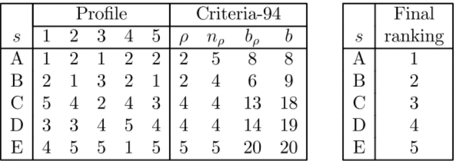
Formally, the first criterion is the median rank ρ (s) of each skater s, that is, the smallest rank such that a majority of judges have placed skater s at one of the ranks 1, . . . , ρ (s) (par. 1, 2, 6)14: the smaller the median rank the better. If two skaters, say s and t, obtain the same median rank, one tries to break the tie by reverting to the numbers of judges nρ(s)
and nρ(t) who gave the median or a better rank to s and t respectively (par. 3): the more
the better. If this is not sufficient to break all ties, one then tries to do so by using the sum of ranks of tied skaters according to the judges who gave the median rank or a better rank to these competitors (par. 4). For skater s, this number is written as bρ(s): the smaller the
better. If there still remains some ties after applying this third criterion, one uses the sum of ranks given to s by all judges (par. 5), or equivalently the Borda scores b (s), as a breaking criterion. Finally, if all ties are not resolved after these four principles have been applied, competitors who tie for a rank obtain the same rank (par. 10).
These criteria are defined as follows. First, given a profile X, let: Ji(s) ={j ∈ J : xjs ≤ i} and ni(s) =|Ji(s)|
Then, ρ (s) = min
i∈{1,...,m}i such that ni(s) >
|J| 2 =
n 2,
Next, for the sake of simplicity, we write Jρ(s) = Jρ(s)(s)and nρ(s) = nρ(s)(s)
Finally, let bρ(s) =
P
j∈Jρ(s)
xjs and recall that b (s) =
P
j∈J
xjs.
Note that b(s)
n is the mean rank of skater s while bρ(s)
nρ(s)
is the mean rank of skater s according to the judges of Jρ(s) .Now, for each candidate s ∈ A, define the vector u(s) ∈ R4
by
u(s) = (ρ (s) , n− nρ(s) , bρ(s) , b(s))
and let ≤ be the lexicographic weak order15
on R4. We can now give the definition of the
ISU-94 rule.
14These are the paragraphs of rule 371 of the regulations. They are reproduced in Truchon (2004). 15Let us first define < . For a, b ∈ RL, a < b if ∃k ∈ {1, . . . , L} : a
k< bk and al= bl∀l < k.
Definition 7 The ISU-94 rule is the function ISU94: Ln → R defined by: ∀s, t ∈ A : ISUs94(X)≤ ISU 94 t (X)⇔ u(s) ≤ u(t)
ISU94(X) is the ISU-94 ranking.
Note that if u(s) = u(t) for some s and t, then s and t obtain the same rank. Table 2 illustrates the computation of the four criteria of this rule.
Profile Criteria-94 s 1 2 3 4 5 ρ nρ bρ b A 1 2 1 2 2 2 5 8 8 B 2 1 3 2 1 2 4 6 9 C 5 4 2 4 3 4 4 13 18 D 3 3 4 5 4 4 4 14 19 E 4 5 5 1 5 5 5 20 20 Final s ranking A 1 B 2 C 3 D 4 E 5
Table 2: Illustration of the ISU-94 rule
3.2.5 The ISU-98 Rule
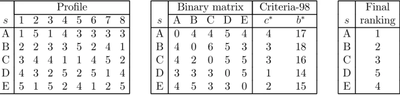
This rule16 represents an important simplification with respect to the ISU-94 rule. Now, skaters are first ranked according to the numbers of other skaters that they defeat according to a majority of judges, or with whom they tie. The Borda rule is once again used to break ties according to the first criterion.17
Formally, let µst:Ln→ R, be a function defined for every pair of alternatives (s, t) and
every profile X, by:
µst(R) = ( 1 if Pnj=1xjst ≥ Pn j=1x j ts 0 otherwise Then, for each alternative s, let:
c∗(s) = X
t∈A\{s}
µst(X)
16This rule is described and illustrated in Communication No. 997 of the ISU, available on the web site
www.isu.org.
17This combination of the Copeland and the Borda rules is all the more curious that they may rank
This number is the Copeland score of s. This is the number of alternatives over which s gets a strict majority of votes or with which it ties.18 Let v(s) = (c∗(s) , b∗(s)) .The formal definition of the ISU-98 rule is the following.
Definition 8 The ISU-98 rule is the function ISU98:Ln → R defined by: ∀s, t ∈ A : ISUs98(X)≤ ISUt98(X)⇔ v(s) ≥ v(t)
ISU98(X) is the ISU-98 ranking.
Put simply, skaters are first ranked according to their Copeland scores c∗(s). If two skaters, say s and t, obtain the same Copeland score, one tries to break the tie by comparing the Borda scores b∗(s) and b∗(t). Finally, if all ties are not resolved after the application of
these two criteria, that is, if v(s) = v(t) for some s and t, competitors who tie for a rank obtain the same rank. Table 3 illustrates the application of this rule. Note that we use the binary matrix hPnj=1xjst
i
s,t∈A as the starting point since we can easily compute the number
of wins under the majority rule from this matrix. Accordingly, b∗ instead of b is the breaking
criterion. Recall that b∗(s) + b(s) = mn.
Profile s 1 2 3 4 5 6 7 8 A 1 5 1 4 3 3 3 3 B 2 2 3 3 5 2 4 1 C 3 4 4 1 1 4 5 2 D 4 3 2 5 2 5 1 4 E 5 1 5 2 4 1 2 5
Binary matrix Criteria-98 s A B C D E c∗ b∗ A 0 4 4 5 4 4 17 B 4 0 6 5 3 3 18 C 4 2 0 5 5 3 16 D 3 3 3 0 5 1 14 E 4 5 3 3 0 2 15 Final s ranking A 1 B 2 C 3 D 5 E 4
Table 3: Illustration of the ISU-98 rule
18Strictly speaking, the Copeland rule is defined with:
µst(X) = 1 if Pnj=1xjst> Pn j=1x j ts 1 2 if Pn j=1x j st= Pn j=1x j ts 0 otherwise
3.3
Loss functions
We use the family of parametric loss functions presented in Gordon and Truchon (2007): dηθ(r, ˆr) =X t∈A Ã X t∈A γst(r, ˆr) !η (m− rs+ 1)θ, η ≥ 0, θ ≥ 0 (9)
Note that d1,0 is the Kemeny metric. With the convention 00 = 0, d00 is the naive or
degenerate distance dN defined by
dN(r, ˆr) = (
κ if ˆr6= r 0 if ˆr = r for some κ > 0.
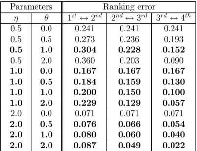
In order to get some intuition for plausible choices of η and θ, we consider the case where there are m = 4 alternatives. The errors associated with incorrectly reversing the first- and second-ranked, the second- and third-ranked and the third- and fourth-ranked alternatives are presented in Table 4. In order to keep a common scale, the loss associated with reversing the true order (that is, getting each of the 28 possible pairwise rankings wrong) is normalized to 1. In our judgement, the combinations in bold reflect the most plausible range of variation in the loss function parameters in (9), except maybe those for which η = 2; see Gordon and Truchon (2007) for a more detailed discussion. However, we retain the combinations with η = 2,in order to test for the robustness of the results to the value of η. We also include the naive distance, represented by d00.
3.4
Simulation methodology
Without loss of generality, the simulations are done under the assumption that the true order is r = (1, 2, . . . , m) . Thus, we may drop r from fαβ(· |r) and dηθ(r, · ) , and write the risk defined in (5), that is, the ex ante expected loss of an aggregation rule Γ, given fαβ and dηθ, as:
ρ¡Γ; fαβ, dηθ¢= X
X∈Ln
fαβ(X)dηθ(Γ (X)) (10) Computing the risk in (10) associated with a given aggregation rule using purely ana-lytical techniques requires evaluating fαβ(X)
at every profile in Ln, and is only feasible for
low-dimension problems, that is, with a small number of alternatives and few judges. In this study, we use Monte Carlo sampling techniques to estimate the population expectation in (10). In each experiment, we choose:
Parameters Ranking error η θ 1st ↔ 2nd 2nd↔ 3rd 3rd ↔ 4th 0.5 0.0 0.241 0.241 0.241 0.5 0.5 0.273 0.236 0.193 0.5 1.0 0.304 0.228 0.152 0.5 2.0 0.360 0.203 0.090 1.0 0.0 0.167 0.167 0.167 1.0 0.5 0.184 0.159 0.130 1.0 1.0 0.200 0.150 0.100 1.0 2.0 0.229 0.129 0.057 2.0 0.0 0.071 0.071 0.071 2.0 0.5 0.076 0.066 0.054 2.0 1.0 0.080 0.060 0.040 2.0 2.0 0.087 0.049 0.022
Table 4: Loss function parameters and implications for costs of errors i) a number of alternatives m ∈ {3, 4, 5, 6, 7, 8, 9, 10, 12, 20},
ii) a number of judges n ∈ {3, 9},
iii) a combination of parameters for the probability function from Table 1,
iv) a combination of parameters for the loss function from those in bold in Table 4. We then simulate K profiles from the chosen statistical model. More precisely, for each voter j and each pair of alternatives (s, t) such that s < t, we draw u ∈ [0, 1] from a uniform distribution. If u < pαβst ,we set ν
j
st = 1 and ν j
ts = 0. Otherwise, we set νist = 0 and ν j ts= 1.
Draws that do not correspond to an order are discarded. We repeat the process for each judge, to obtain a profile X. Repeating K times yields a sample Ωαβmn.
In a second step, we apply the aggregation rules described in subsection 3.2, that is, the ISU-94, the ISU-98, the Borda, and the Kemeny rules19 to each profile. With 3 to 6
(sometimes 7) alternatives, we also apply the maximum likelihood rule M L³· , ˆα, ˆβ´.20 We
19The ISU-94, the ISU-98 and the Borda rules yields a unique ranking. However, there may be more than
one Kemeny order. In this case, the mean Kemeny ranking, defined in the Appendix, has been retained when it existed. Otherwise, a ranking close to the Copeland ranking has been chosen.
20As is the case for the Kemeny rule, there may be more than one maximum likelihood order. The mean
maximum likelihood ranking has been retained when it existed. Otherwise, a ranking close to the chosen Kemeny ranking has been retained. See the Appendix for more on this point.
always start with³α, ˆˆ β´= (α, β)but we also try other values of ˆβto check for the robustness of the rule.21
These four of five rules make up the set G. Finally, for each rule Γg
∈ G and each loss function dηθ, we compute the statistic:
ˆ ρ(Γg; Ωαβmn, dηθ) = 1 K X X∈Ωαβmn dηθ(Γg(X)) (11)
This statistic is a simulation-consistent estimator for the risk associated with a given ag-gregation rule. The value of K is set so that the standard errors are below 1% (2% in one subset of simulations) of their corresponding estimates.
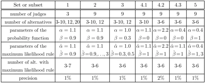
Five sets of simulations were performed. In the first, the number of judges is 3 and the number of alternatives ranges from 3 to 10 and then jumps to 12 and 20. The values of the parameters for simulating the votes are α = 1.1 and β = 0.9. In the second, the number of judges is raised to 9, as in figure skating, and the the number of alternatives ranges from 3 to 10 and 12. The third set is similar to the second, except that α = 1 and β = 0.3. In the fourth set, β = 0 and three different values are used for α, namely 1.1, 2.2 and 0.4. The number of alternatives ranges from 3 to 10 when α = 1.1 and from 3 to 6 otherwise. In the last set, α = 0.4 and β = 1, that is, we go back to variable probabilities, but with a lower competency for the judges. The respective characteristics of the five sets of simulations are given in Table 5. Note that the fourth set is broken into three subsets.
21The set of maximizers of the likelihood function is invariant to a multiplication of³α, ˆˆ β´by a positive
scalar γ. Thus, we vary only ˆβ. However, the choice of the absolute values of the parameters α and β in the vote generating function is not innocuous. The larger these values, the larger the probabilities of correctly ordering two alternatives, the larger the probability that a judge selects the true ranking or at least a ranking close to the true one, and the smaller the probability of a cycle in her vote.
Set or subset 1 2 3 4.1 4.2 4.3 5 number of judges 3 9 9 9 9 9 9 number of alternatives 3-10, 12, 20 3-10, 12 3-10, 12 3-10 3-6 3-6 3-6 parameters of the probability function α = 1.1 β = 0.9 α = 1.1 β = 0.9 α = 1.0 β = 0.3 α = 1.1 β = 0 α = 2.2 β = 0 α = 0.4 β = 0 α = 0.4 β = 1 parameters of the maximum likelihood rule
ˆ α = 1.1 ˆ β = 0.9 ˆ α = 1.1 ˆ β = 0.9,. . ., 3 ˆ α = 1.0 ˆ β = 0.3, 0.5 ˆ α = 1.1 ˆ β = 1 ˆ α = 2.2 ˆ β = 1 ˆ α = 1.1 ˆ β = 1 ˆ α = 0.4 ˆ β = 1, 3
number of alt. with
maximum likelihood rule 3-7 3-6 3-6 3-6 3-6 3-6 3-6
precision 1% 1% 1% 1% 2% 1% 1%
Table 5: Description of the simulations
4
The results in brief
In assessing the behavior of the different rules, four facts should be taken into account: • ML (0) and the Kemeny rule coincide,
• ML³βˆ´ and the Borda rule coincide when ˆβ = ˆα, which, in our case, means ˆβ = α,22
• the Kemeny and the ISU-98 rules are both Condorcet consistent, that is, they select the Condorcet order when it exists;23 thus, we can expect them to give similar results,
• ML³βˆ´ should do best with ˆβ = β and thus, M L be decreasing from 0 to β and increasing afterward.
As it turned out, M L³βˆ´ did best, not only in the M L family, but against all other rules, with a minor exception24. Because of the four facts mentioned above, the relative
position of the Borda, the Kemeny and the ISU-98 rules, in terms of expected loss, depends on the relative values of α and β. So do the relative position of the Borda and the ISU-94 rules and the discrepancy between the Borda and the M L (β) rules. A priori, we cannot say much about the ISU-94 rule.
22This assertion is proved in Truchon (2006) under the hypothesis that a subset of most likely orders
that differ only by the permutation of adjacent alternatives, are replaced by a single ranking in which these alternatives tie.
23It is well known that the Borda rule is not Condorcet consistent. The ISU-94 rule is not either. See
Remark 5 in Truchon (2004) for a proof.
24The exception is for the case (α, β) = (1.0, 0.3) and η = 2. See Table 11 in Appendix B. The explanation
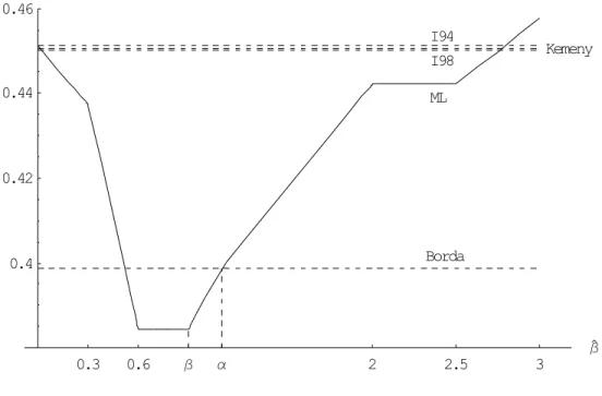
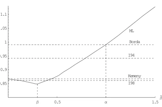
Figures 1 to 4 illustrate four typical behaviors. Expected losses are those obtained for six alternatives, nine judge and η = θ = 1. The figures have been drawn from a few values of ˆβ, hence the lack of smoothness. From these figures, we note the following:
• When β (the rate of increase in the probability) is large, ML (0) is large compared to M L (β) .Thus, the Kemeny and the ISU-98 rules give large and similar expected losses since M L (0) and the Kemeny rule coincide and since the Kemeny and the ISU-98 rules are both Condorcet consistent. This is the case in Figures 1 and 2. The ISU-94 rule fares better than the Kemeny and the ISU-98 rules in one case and slightly worst in the other.
• When β is low, as in Figures 3 and 4, ML (0) is close to ML (β) . Thus, the Kemeny rule yields an expected loss close to what M L (β) gives. As a consequence, it does almost25 always better than the maximum likelihood rule. The ISU-98 rule is the only
one that does better but by a very small margin. Then, the chance is high that the ISU-94 rule will give a larger expected loss, as is the case in these two figures. The Borda rule does worst due to the facts that β < α and that M L is an increasing function past β.
• When α and β are close to each other, as in Figure 2, the Borda rule fares well since it has an expected loss close to M L (β) , which is the smallest of all. This leaves little room for the other rules. Thus, the chances are that the two ISU and the Kemeny rules give a much larger expected loss than all others, except M L³βˆ´ for values of ˆβ far from β. This is what we observe in Figure 2.
• The Borda rule may also fare relatively well when β is much larger than α, as in Figure 1, provided that α is large enough, which it must be for the probability of correctly ordering two alternatives to be larger than one half. The performance of the maximum likelihood rule also appears to be robust to the value of ˆβ above β.
• When α is much larger than β, as in Figures 3 and 4, the Borda rule yields a large expected loss, compared to M L (β) . The reason is that the Borda rule coincides with M L (α) but, when ˆβ reaches α, the expected loss given by M L has increased by a large amount. Typically, all other rules will do better than Borda, except M L³βˆ´for ˆ
β > α.
Appendix B presents a full description of the simulations. Here are a few additional points that are worth mentioning here.
• The few simulations that were done with three judges generated results that are sometimes quite different from those obtained with nine judges. For example, with (α, β) = (1.1, 0.9) and less than 6 alternatives, the Borda rule produces the largest expected loss of all rules. Its performance improves as the number of alternatives increases. With 8 alternatives and more, it becomes the best rule.
• Setting η = 2 improves the performance of the Borda rule. The reason is that most errors under the Borda rule consist in declaring ex aequo two adjacent alternatives in the true order and that kind of error is worth a penalty of 12 compared to 1 for an inversion. These penalties entering the function ( · )η, the result is a lower expected loss with η = 2 than with η = 1.
• Except for the Borda rule, the value of θ has an important impact on the expected losses but not on the rankings of the rules in terms of these losses. This may be an indication that, under all rules, most errors involve essentially the same alternatives or close alternatives in the true order. Increasing θ from 1 to 2 is often beneficial to the Borda rule. This is an other indication that this rule often produces ties between alternatives.
5
Conclusion
If it is supposed that a true social order exists, but that individual voters observe it with error, then the social choice problem is one of optimal inference. This study - along with the companion paper of Gordon and Truchon (2007) - formalises and extends Condorcet’s framework in two directions. Firstly, we make the choice-theoretic nature of the problem more explicit by specifying a loss function that describes the consequences of choosing an incorrect social ranking. Secondly, we extend the usual constant-probability case to one in which voters find it easier to distinguish alternatives that are far apart, and more difficult to correctly order similar alternatives.26
This study develops a statistical procedure for the ex ante evaluation of vote aggrega-tion rules. In our Monte Carlo applicaaggrega-tion, we specify both the distribuaggrega-tion funcaggrega-tion that
26In Gordon and Truchon (2007), there is actually a third extension that consist in taking into account the
generates individual votes and a loss function that can be used to evaluate the expected loss associated with a given decision rule.
We find that the maximum likelihood (ML) rule, with the correct form and the true parameters of the vote distribution function, generally outperforms its competitors, that is, the Borda, the Kemeny and two rules that have been used for many years in figure skating. Moreover, ML seems to be somewhat robust to the value of ˆβ when α is small. However, its feasibility in real-world applications, where the form and the parameters of the distribution function are not known, is limited. In addition, the computational burden forbids the use of ML with a large number of alternatives, such as in figure skating.
The performance of the other rules varies considerably with the value of the parameters of the probability function used to generate the votes. For example, the Borda rule does well with increasing probabilities but poorly with constant probabilities. It appears that no single vote aggregation rule can be expected to perform best in all circumstances.
α β 2 3 5 β ˆ 1.2 1.4 1.6 1.8 2 2.2 I94 I98 Kemeny Borda ML
Figure 1: Typical expected losses as a function of ˆβ when α = 0.4 and β = 1
β α 0.3 0.6 2 2.5 3 β ˆ 0.4 0.42 0.44 0.46 I94 I98 Kemeny Borda ML
α β 0.5 1.5β ˆ 0.85 0.9 0.95 1 1.05 1.1 I94 I98 Kemeny Borda ML
Figure 3: Typical expected losses as a function of ˆβ when α = 1 and β = 0.3
α 0.1 0.3 0.5 1 1.2 1.5 β ˆ 1 1.2 1.4 1.6 1.8 I94 I98 Kemeny Borda ML
Appendices
A
Finding Kemeny orders and choosing among them
Finding a Kemeny order by considering all possible permutations of the skaters, as the definition suggests, may prove prohibitive when the number of competitors is large as in figure skating. There are many contributions in the literature that address this specific problem.27 Whatever the method used, Truchon (2004) shows that one way to ease the task it to break the problem into many subproblems, using an extension of Condorcet Consistency that he calls the Extended Condorcet Criterion (XCC). In essence, this criterion says that if the set of alternatives can be partitioned in such a way that all members of a subset of this partition defeat all alternatives belonging to subsets with a higher index, then the former should obtain a better rank than the latter. Such a partition is called a Condorcet partition. The finest Condorcet partition can be found by first ordering alternatives according to another rule that satisfies XCC, such as the Copeland rule. For most practical applications, a Kemeny order on each subset of the finest Condorcet partition can be found by simple enumeration. Then, a complete Kemeny order is obtained by juxtaposing the Kemeny orders on the subsets of the partition. This is the approach adopted in our study. However, this approach does not extend to the M L rule since this rule does not satisfy XCC. For this reason, we have to limit the number of alternatives to 6 or 7 when applying this rule.
The Kemeny rule may yield more than one order. This occurrence can sometimes be resolved by reverting to the concept of the mean Kemeny ranking also taken from Truchon (2004). Given a set of Kemeny orders©rˆ1, . . . , ˆrkª, consider the weak order ˜r defined by:
∀s, t ∈ A : ˜rs ≤ ˜rt⇔ k X q=1 ˆ rqs ≤ k X q=1 ˆ rqt
This weak order is a ranking according to the mean ranks of alternatives over all Kemeny orders. It will be called the mean Kemeny ranking if and only it weakly agrees with at least one order in ©rˆ1, . . . , ˆrkª, that is, if there exists an order ˆrq
∈©rˆ1, . . . , ˆrkªsuch that:
∀s, t ∈ A : ˆrsq < ˆr q
t ⇒ ˜rs ≤ ˜rt
We may define a mean ML ranking in a similar manner.
27Several of these contributions are based on mathematical programming. See Truchon (2004) for some
B
Description of the results
The complete results of the simulations, that is, the expected losses, are available upon re-quest from the authors. Here, we only present the main highlights of these results. There are five subsections corresponding to the five sets of simulations. In the tables of this appendix, the notation Y ≺ Z stands for rule Y yields a lower expected loss than rule Z, Y ∼ Z means that the expected losses are the same under Y and Z, and B, K, I94, I98 represent the Borda,
the Kemeny, the ISU-94 and the ISU-98 rules respectively. M L represents the maximum likelihood rule with³α, ˆˆ β´= (α, β) while M L³βˆ´represents the same rule for the specified value of ˆβ and for ˆα = α.
B.1
Simulations with three judges and
(α, β) = (1.1, 0.9)
The main highlights of these simulations are:
• Save the Borda rule, increasing η has a relatively small effect on the expected loss. This is an indication that most errors consist in inverting adjacent alternatives in the true order.
• In the case of Borda, the impact of increasing η is also small but it goes in the reverse direction. It causes the expected error to decrease. This is a confirmation that most errors consist in declaring ex aequo two adjacent alternatives in the true order. Recall that tying two adjacent alternatives is worth a penalty of 1
2 compared to 1 for an
inversion, hence the decrease in the size of the error as the parameter η increases. • The Borda rule always produces the largest proportion of erroneous rankings. This
translates into the worst expected loss for this rule when (η, θ) = (0, 0) or (12, 1). But, for η = 2, the expected loss is always smaller under this rule than under any other rule, for the reason given above.
• Table 6 shows the relation between the different rules for the other values of the para-meters, that is, (η, θ) = (1, 0) ,¡1,12¢, (1, 1) , (1, 2) .
• From this table, one can note that, for 3 alternatives, all rules other than Borda give the same expected losses.
• With the number of alternatives ranging from 4 to 7, the expected loss is always smaller under the maximum likelihood rule than under any other rule. This was to be expected since this rule incorporates the hypothesis used in generating the profiles.
Alternatives Relations between rules 3 M L∼ I98 ∼ I94 ∼ K ≺ B 4-5 M L≺ I98 ≺ I94 ≺ K ≺ B 6 M L≺ I98 ≺ B ≺ I94≺ K 7 M L≺ B ≺ I98≺ I94≺ K 8-20 B ≺ I98 ≺ I94 ≺ K
Table 6: Relation between different rules in terms of expected loss with 3 judges and η = 1 • As we increase the number of alternatives, the Borda rule gets a better position with
respect to the other rules. The relation between the other rules does not change. Given that the ISU-98 and the Kemeny rules are both Condorcet consistent while the ISU-94 is not, the fact that the ISU-94 rule gives expected losses between those obtained with the two others is somewhat puzzling. However, it must be said that the two ISU and the Kemeny rules produce results that are not markedly different from one another. • In terms of the naive distance, the order between the two ISU and the Kemeny rules
is not always the one described above. This is also often the case with η = 12. This illustrates the usefulness of a more subtle distance between rankings.
• For (η, θ) =¡2,1 2
¢
, (2, 1) , (2, 2) ,the relations of Table 6 are changed by simply moving the Borda rule at the head.
• Increasing θ has an important impact on the expected losses but not on the rankings of the rules in terms of these losses.
• The expected loss under all loss functions increases with the number of alternatives as there is more scope for errors from the judges. The standard error also increases with the number of alternatives but not in proportion to the expected loss, especially for the naive distance. As a consequence, the size of the sample to meet 1% precision decreases with the number of alternatives.
• Table 7 gives the theoretical probabilities of cycles (rounded to 3 digits) for 3 to 10 alternatives and the observed fractions of cycles in the simulations.28 As expected,
they are close to each other. For 12 alternatives, we give only the observed fractions of cycles since computing the theoretical probability is prohibitive in this case.
Number of alternatives 3 4 5 6 7 8 9 10 12 Probability of cycles 0.122 0.273 0.411 0.527 0.622 0.698 0.759 0.8075
Frequency of cycles 0.121 0.274 0.409 0.527 0.622 0.698 0.759 0.8081 0.878 Table 7: Probabilities and empirical frequencies of cycles with α = 1.1, β = 0.9
B.2
Simulations with nine judges and
(α, β) = (1.1, 0.9)
The main highlights of these simulations and the main differences with those of three judges are:
• The expected losses are markedly smaller than the corresponding losses with three judges. Condorcet (1785) showed that the larger the number of judges, the higher the probability that the majority rule under the binary approach yields the true order. In as much as the ISU-98, the Kemeny and the maximum likelihood rules respect the view of the majority on each pair of alternatives when these views are consistent, these results are not surprising at least for these rules.
• The standard errors are also smaller than the corresponding ones with three judges but the diminution is not as marked as it is for the means. Hence, larger samples have been required to meet 1% precision.
• The behavior of the Borda rule with respect to the parameter η is similar to what we observed with three judges. It is also similar for the other rules, except that, this time, the ISU-94 rule behaves more like the Borda rule, producing a lower expected loss as η increases. This is an indication that, with these two rules, most errors consist in declaring ex aequo two adjacent alternatives in the true order.
• For less than seven alternatives, the maximum likelihood rule has been applied with more than one pair of values for the parameters. This allows us to test for the robustness of this rule with respect to its parameters.
• Table 8 shows the relation between the rules for (η, θ) = (1, 0) ,¡1,12¢, (1, 1) , (1, 2) . • For (η, θ) =¡2,12¢, (2, 1) , (2, 2) ,the relations of Table 8 are changed by simply moving
the Borda rule at the head in the cases of 3 to 6 alternatives.
• It can be observed that, when applied, the maximum likelihood rule with ³α, ˆˆ β´ = (α, β) gives expected losses smaller than any other rule. However, its performance deteriorates as ˆβ is increased above β.
Alternatives Relations between rules 3 M L (0.9)≺ B ≺ ML (1.5) ≺ I94≺ I98≺ K ≺ ML (1.75) ∼ ML (2) 4 M L (0.9)≺ B ≺ I94≺ ML (2) ∼ ML (2.5) ≺ I98≺ K ≺ ML (3) 5 M L (0.9)≺ B ≺ ML (1.5) ≺ I94≺ I98≺ K ≺ ML (1.75) 6 M L (0.9)≺ B ≺ ML (2) ∼ ML (2.5) ≺ I94≺ I98≺ K ≺ ML (3) 7-10, 12 B ≺ I94 ≺ I98 ≺ K
Table 8: Relation between different rules in terms of expected loss, α = 1.1, β = 0.9, η = 1 • With 3 and 5 alternatives and ˆβ = 1.5, the maximum likelihood rule gives a better
result than all other rules, save the Borda rule. With ˆβ = 1.75,the expected loss under the maximum likelihood rule becomes worst than under all other rules. With 4 and 6 alternatives, we have the same kind of pattern but with ˆβ = 2.5 and 3 instead of 1.5 and 1.75 respectively. Thus, the deterioration of the maximum likelihood rule arises for a larger value of ˆβ. It would be interesting to know if this difference is typical of the odd and even numbers of alternatives but we did not apply the maximum likelihood rule for larger numbers of alternatives.
• Turning to larger numbers of alternatives (≥ 7), the ISU-94 rule does slightly better than the ISU-98 and the latter does slightly better than the Kemeny rule. This order is different from the one observed with three judges. However, the differences are not marked, specially between the ISU-98 and the Kemeny rules.29 Again, these two rules
being Condorcet consistent, it is not surprising that they give similar results. What is more surprising is that the ISU-94 does better. Note that the relation between the rules also holds for (η, θ) = (12, 1) when there are more than six alternatives. This is not the case with the naive distance.
• Increasing θ has again an important impact on the expected losses but not on the rankings of the rules in terms of these losses.
• For 3 alternatives, different rules give different expected losses, contrary to what we had with 3 judges.
• What was said about expected losses, standard errors and the size of the samples with respect to the number of alternatives, with three judges, remains true with nine judges.
29However, the difference in the expected losses is, most of the time, significant with a high degree of
• The theoretical probabilities of cycles are of course the same and the empirical fre-quencies sensibly the same.30
B.3
Simulations with nine judges and
(α, β) = (1.0, 0.3)
The main highlights of these simulations and the main differences with the preceding are: • The competency of the judges being lower, their votes are more erratic, resulting in
larger expected losses, roughly twice as large as those obtained with (α, β) = (1.1, 0.9) . • The standard errors are also larger but the increase is not as marked as it is for the
means. Hence, smaller samples have been required to meet 1% precision.
• As a result of the lower competency of the judges, the theoretical probabilities of cycles and the empirical frequencies are considerably larger.31 See Table 9.
Number of alternatives 3 4 5 6 7 8 9 10 12 Probability of cycles 0.171 0.428 0.657 0.815 0.908 0.957 0.980 0.992
Frequency of cycles 0.171 0.427 0.656 0.815 0.908 0.956 0.981 0.992 0.999 Table 9: Probabilities and empirical frequencies of cycles with α = 1, β = 0.3 • Table 10 shows the relation between the rules for (η, θ) = (0, 0) ,¡12, 1
¢
, (1, 0) ,¡1,12¢, (1, 1) , (1, 2) . Here, M L³βˆ´ represents the maximum likelihood rule for the specified value of ˆβ and for ˆα = 1.
• The ∗ indicate exceptions:
— For 4 to 6 alternatives and the pair (η, θ) = (0, 0) , the relation between M L (0.5) and I94 is inverted.
— For 9 alternatives and the pairs (1, 0) , ¡1,12¢, the relation between I94 and B is
inverted.
— For 10 and 12 alternatives and the pairs (1, 0) , ¡1,12¢, (1, 1) ,the relation between I94 and B is inverted.
30To give an example of the impact of the possibility of cycles in individual rankings, with 9 judges and
10 alternatives, close to 5 millions of binary matrices have been drawn in order to obtain 105 000 polls of consistent rankings (orders).
31As a result, with 12 alternatives, more than 209 millions of binary matrices have been drawn in order
Alternatives Relations between rules
3 M L (0.3)≺ I98 ≺ K ≺ ML (0.5) ≺ I94 ≺ B ≺ ML (1.5)
4-6 M L (0.3)≺ I98≺ K ≺ ML (0.5) ≺∗ I94≺ B ≺ ML (1.5)
7-8 I98≺ K ≺ I94 ≺ B
9-10, 12 I98 ≺ K ≺ I94≺∗ B
Table 10: Relation between different rules in terms of expected loss, α = 1, β = 0.3, η 6= 2 • There is a striking difference between the above relations and those of Table 8 obtained
with (α, β) = (1.1, 0.9) . The Borda rule, which was the second best performer, after the maximum likelihood rule with³α, ˆˆ β´= (α, β) ,is now the worst. The ISU-94 rule also gives worst results and becomes the second worst.
• Again, when applied, the maximum likelihood rule with³α, ˆˆ β´= (α, β)gives expected losses smaller than any other rule. However, its performance deteriorates as ˆβ is increased above β. It becomes worst than Kemeny with ˆβ = 0.5 and worst of all with ˆ
β = 1.5.
• Table 11 shows the relation between the rules for (η, θ) =¡2,1 2
¢
, (2, 1) , (2, 2) . Alternatives Relations between rules
3 M L (0.5)≺ B ≺ ML (0.3) ≺ I98 ≺ K ≺ I94 ≺ ML (1.5)
4-6 M L (0.5)≺ ML (0.3) ≺ I98≺ K ≺ B ≺ I94 ≺ ML (1.5)
7 I98≺ K ≺ B ≺ I94
8-10, 12 B ≺∗ I98≺ K ≺ I94
Table 11: Relation between different rules in terms of expected loss, α = 1, β = 0.3, η = 2 • There are two exceptions as indicated by the ∗ : For 9 and 12 alternatives and (η, θ) =
(2, 2) , the relation between B and I98 is inverted.
• With η = 2 instead of 1, the performance of the Borda rule improves. This rule jumps to the first place for 8 alternatives and more. The improvement is marginal for 4 to 7 alternatives. The performance of M L (0.5) also improves to the point of becoming the best of all, even better that M L (0.3) .
• The reason for the better performance of ML (0.5) and B when η = 2 is due to the fact that these two rules produce more ties than the other rules. For example, in the case of 3 alternatives, the first 200 profiles produced more errors in the M L (0.5) ranking than in M L (0.3) but 3 of the errors under M L (0.5) were ties while there were no ties under M L (0.3) . Since the penalty entering the function ( · )η is 12 for a tie instead of 1,the result is a lower expected loss with η = 2 than with η = 1.
B.4
Simulations with nine judges and a constant probability
In the preceding subsections, we saw that the maximum likelihood rule with³α, ˆˆ β´= (α, β) does better than the Kemeny rule, with the minor exception mentioned in the last point above. Recall that the Kemeny rule is the maximum likelihood rule with ˆβ = 0. However, increasing ˆβ above β causes the performance of the maximum likelihood rule to deteriorate. At some point, it becomes worst than that of the Kemeny rule. We now examine three subsets of simulations where votes are generated with constant probabilities, that is, β = 0. Simulations with a constant probability of 0.75
In the first subset of simulations, the votes have been cast with α = 1.1 and β = 0. This means that the probability of correctly ordering two alternatives is 0.75, the same as the probability of correctly ordering two adjacent alternatives with α = 1.1 and β = 0.9. The maximum likelihood rule has been applied with ˆα = 1.1 and ˆβ = 0.1, 0.3, 0.5, 1.0. The main highlights of these simulations and the main differences with the preceding are:
• Keeping the probability constant means that judges vote in a more erratic way, which translates into larger expected losses compared to those with α = 1.1 and β = 0.9. With 3 alternatives, the expected losses are almost twice as large as those with in-creasing probabilities. The deterioration is slightly worst for the Borda rule. With 6 alternatives, they are more than twice as large, and almost three times for the Borda rule.
• Except for the case of three alternatives, expected losses are also larger than those obtained with α = 1 and β = 0.3 and the difference increases with the number of alternatives. The increase is more marked for the Borda rule. For three alternatives, expected losses under the Borda rule are also larger than those obtained with α = 1 and β = 0.3 but they are smaller for all other rules.
• For 4 to 6 alternatives, the relation between the rules, in terms of expected loss, is the following for all values of η and θ, with two minor exceptions:
I98≺ K ≺ ML (0.3) ≺ ML (0.5) ≺ I94 ≺ ML (1) ≺ B ≺ ML (1.2)
The two minor exceptions concern the relation I98 ≺ K in the case of 4 alternatives.
It becomes I98 ∼ K when η = 0 and K ≺ I98 when η = 12.
• For 3 alternatives, this relation is changed by moving ML (0.3) ahead of K when η = 2 and by having both rules tie when η = 1.
• Introducing ML (0.1) into the picture has the following impact. In the case of 3 alternatives, M L (0.1) gives exactly the same expected loss as K. For 4 to 6 alternatives, M L (0.1)comes between I98 and K and sometimes before I98 depending on the values
of η and θ.
• Thus, contrary to what was to be expected, the maximum likelihood rule with a low value of ˆβ (0.1 or 0.3) gives a slightly better result than the Kemeny rule. As far as we can see, this is due to the handling of multiple rankings produced by the two rules. However, the performance of the ML rule gets worst as ˆβ increases. With ˆβ = 0.5, it is still better than that of the ISU-94 rule but it gets worst than the latter, yet with ˆ
β = 1, it remains better than the Borda rule. • For 7 to 10 alternatives, the relation is
I98 ≺ K ≺ I94≺ B
except that I98Â K when there are 7 and 8 alternatives.32
• The above relations are similar to those obtained with (α, β) = (1.0, 0.3) and η = 1. The striking fact is that they remain the same with η = 2, due to the bad behavior of the Borda rule.
Simulations with a constant probability of 0.9
In the second subset, the votes have been cast with α = 2.2 and β = 0, that is, with a constant probability of 0.9. This high probability results in more votes that are identical to
32In the case of 9 alternatives, half a billion of binary matrices have been drawn in order to obtain 36 000
polls of consistent rankings (orders). For 10 alternatives, only 2 278 polls have been generated after four days of computing, due to the very high frequency of cycles. Hence, the precision is only 3.4%.
the true order. As a result, all rules select the true order most of the time. The fraction of erroneous rankings is less than 1%, with one exception. The Borda rule is again and by far the worst performer. The maximum likelihood rule has been applied with ˆα = 2.2 and ˆ
β = 1 or, equivalently, ˆα = 1.1 and ˆβ = 0.5. Thus, the rate of increase in the probabilities is weak. Yet, in all cases, the Kemeny rule gives a lower expected loss than the maximum likelihood rule. The relation between the rules in terms of expected losses is the following for the four numbers of alternatives considered and all values of η and θ :
I98∼ K ≺ ML (0.5) ≺ I94≺ B
This relation indicates that the Kemeny and the ISU-98 rules give expected losses that are equal or not significantly different. The explanation is straightforward. Most votes being identical to the true order, there is a Condorcet order with most profiles and both rules being Condorcet consistent, select this order.
This subset of simulations has been done with a precision of 2% instead of 1%. As remarked before, the lower the expected loss, the larger the number of profiles required to achieve a given degree of precision. The reason is that the variance does not decrease proportionally to the expected loss. In this case, more than one million of draws have been necessary to achieve a precision of 2%. These numbers would have had to be multiplied by 4 to achieve a precision of 1%.
Simulations with a constant probability of 0.6
In the third subset, the votes have been cast with α = 0.4 and β = 0, that is, with a constant probability of 0.6. This means that the competency of the judges in assessing the true order is very low. As a result, all rules do badly in terms of the expected losses. One cannot ask rules to aggregate bad votes into something close to the true order. With three alternatives, all rules miss the true order more than 50% of the time. With six alternatives, this percentage is higher. With the naive distance, the relation between the rules is:
I98 ≺ K ≺ ML (1) ≺ I94≺ B
However, this relation varies when a more general distance is used and it also changes with the values of the parameters. In short, everything is more erratic in this case.
B.5
Simulations with nine judges and
(α, β) = (0.4, 1)
In the preceding subsection, we saw that lowering β could have a non-negligible impact on the relative performances of the rules. The impact was most important for the Borda rule,