Maximum Likelihood and the Bootstrap for Nonlinear Dynamic Models

Montréal

Avril 2002

Série Scientifique

Scientific Series

2002s-41

Maximum Likelihood and the

Bootstrap for Nonlinear

Dynamic Models

Sílvia Gonçalves, Halbert White

CIRANO

Le CIRANO est un organisme sans but lucratif constitué en vertu de la Loi des compagnies du Québec. Le financement de son infrastructure et de ses activités de recherche provient des cotisations de ses organisations-membres, d’une subvention d’infrastructure du ministère de la Recherche, de la Science et de la Technologie, de même que des subventions et mandats obtenus par ses équipes de recherche.

CIRANO is a private non-profit organization incorporated under the Québec Companies Act. Its infrastructure and research activities are funded through fees paid by member organizations, an infrastructure grant from the Ministère de la Recherche, de la Science et de la Technologie, and grants and research mandates obtained by its research teams.

Les organisations-partenaires / The Partner Organizations

•École des Hautes Études Commerciales •École Polytechnique de Montréal •Université Concordia

•Université de Montréal

•Université du Québec à Montréal •Université Laval

•Université McGill

•Ministère des Finances du Québec •MRST

•Alcan inc. •AXA Canada •Banque du Canada

•Banque Laurentienne du Canada •Banque Nationale du Canada •Banque Royale du Canada •Bell Canada

•Bombardier •Bourse de Montréal

•Développement des ressources humaines Canada (DRHC) •Fédération des caisses Desjardins du Québec

•Hydro-Québec •Industrie Canada

•Pratt & Whitney Canada Inc. •Raymond Chabot Grant Thornton •Ville de Montréal

© 2002 Sílvia Gonçalves et Halbert White. Tous droits réservés. All rights reserved. Reproduction partielle permise avec citation du document source, incluant la notice ©.

Short sections may be quoted without explicit permission, if full credit, including © notice, is given to the source.

ISSN 1198-8177

Les cahiers de la série scientifique (CS) visent à rendre accessibles des résultats de recherche effectuée au CIRANO afin de susciter échanges et commentaires. Ces cahiers sont écrits dans le style des publications scientifiques. Les idées et les opinions émises sont sous l’unique responsabilité des auteurs et ne représentent pas nécessairement les positions du CIRANO ou de ses partenaires.

This paper presents research carried out at CIRANO and aims at encouraging discussion and comment. The observations and viewpoints expressed are the sole responsibility of the authors. They do not necessarily represent positions of CIRANO or its partners.

Maximum Likelihood and the Bootstrap

for Nonlinear Dynamic Models

Sílvia Gonçalves

and Halbert White

Résumé / Abstract

Nous proposons une approche unifiée pour analyser la méthode de bootstrap appliquée aux estimateurs de pseudo-maximum de vraisemblance dans le contexte de modèles non linéaires dynamiques où les données sont caractérisées par une dépendance d'époque proche. Nous appliquons nos résultats à la méthode de bootstrap de blocs mouvants de Künsch (1989) et Liu et Singh (1992) et nous démontrons la validité asymptotique de premier ordre de l'approximation du bootstrap à la distribution asymptotique de l'estimateur de pseudo-maximum de vraisemblance. Nous considérons aussi l'application du bootstrap à la réalisation de tests d'hypothèses. En particulier, nous démontrons la validité asymptotique des versions de bootstrap des tests de Wald et du multiplicateur de Lagrange.

We provide a unified framework for analyzing bootstrapped extremum estimators of nonlinear dynamic models for heterogeneous dependent stochastic processes. We apply our results to the moving blocks bootstrap of Künsch (1989) and Liu and Singh (1992) and prove the first order asymptotic validity of the bootstrap approximation to the true distribution of quasi-maximum likelihood estimators. We also consider bootstrap testing. In particular, we prove the first order asymptotic validity of the bootstrap distribution of suitable bootstrap analogs of Wald and Lagrange Multiplier statistics for testing hypotheses.

Mots-Clés : Bootstrap en bloc, pseudo-maximum de vraisemblance, modèle non linéaire

dynamique, dépendance d'époque proche, test de Wald.

Keywords: Block bootstrap, quasi-maximum likelihood estimator, nonlinear dynamic

model, near epoch dependence, Wald test.

* _{We would like to thank Rui Castro and Nour Meddahi for many helpful discussions, and Jeff}

Wooldridge for suggesting the logit example. In addition, we are grateful to numerous seminar participants on earlier versions of this paper, and to three anonymous referees and a co-editor for many valuable suggestions.

† _{C.R.D.E, CIRANO and Université de Montréal, C.P.6128, succ. Centre-Ville, Montréal, QC,}

H3C 3J7, Canada. Tel: (514) 343 6556. Email: silvia.goncalves@umontreal.ca. Gonçalves acknowledges financial support from Praxis XXI and a Sloan Dissertation fellowship.

‡

University of California, San Diego, 9500 Gilman Drive, La Jolla, California, 92093-0508. USA. Tel: (858) 534-3502. Email: hwhite@weber.ucsd.edu. White’s participation has been supported by the National Science Foundation, grants SBR-9811562 and SES 0111238.

1. Introduction

The bootstrap is a powerful and increasingly utilized method for obtaining conÞdence intervals and performing statistical inference. Despite this, results validating the bootstrap for the quasi-maximum likelihood estimator (QMLE) or generalized method of moments (GMM) estimator have previously been available only under restrictive assumptions, such as stationarity and limited memory. A main goal here is thus to establish the bootstrap’s Þrst order asymptotic validity in the framework of Gallant and White (1988) and Pötscher and Prucha (1991): extremum estimators for nonlinear dynamic models of stochastic processes near epoch dependent (NED) on an underlying mixing process. We treat primarily QML estimators for concreteness and because there are fewer results in this area. See Corradi and Swanson (2001) for a treatment of GMM estimation that draws on the results provided here.

We apply our results to the moving blocks bootstrap (MBB) of Künsch (1989) and Liu and Singh (1992). Here, this involves resampling blocks of the quasi-log-likelihood values. With misspeciÞed models, the associated scores are generally dependent, justifying our use of block bootstrap methods.

Results for bootstrapping extremum estimators are available for special cases. For example, Hahn (1996) shows Þrst order asymptotic validity of Efron’s bootstrap for GMM with i.i.d. data. Hall and Horowitz (1996) give asymptotic reÞnements for bootstrapped GMM estimators with stationary ergodic data. Andrews (2001) extends their results, establishing higher-order improvements of k-step bootstrap estimators (see Davidson and MacKinnon (1999)) for nonlinear extremum estimators, including GMM and ML. Both Hall and Horowitz (1996) and Andrews (2001) take the moment conditions deÞning the estimator to be uncorrelated after Þnitely many lags, obviating use of HAC covariance estimators. For stationary mixing processes, Inoue and Shintani (2001) prove asymptotic reÞnements for GMM applied to linear models where the deÞning moment conditions have unknown covariance.

Here, we do not attempt asymptotic reÞnements. Instead, we prove the consistency of the block bootstrap estimator of the QMLE sampling distribution for a broad class of models and data generating processes. SpeciÞcally, we avoid stationarity and restrictive memory conditions, and show that the block bootstrap distribution of the QMLE converges weakly to the distribution of the QMLE. Thus, bootstrap conÞdence intervals have correct asymptotic coverage probability.

for new bootstrap Wald and LM tests. The asymptotic validity of the percentile-t test follows from that of the Wald test, justifying use of MBB to construct percentile-t conÞdence intervals.

We illustrate MBB Þnite sample performance for conÞdence intervals via two Monte Carlo experi-ments. SpeciÞcally, we compute conÞdence intervals for 1) a logit model with neglected autocorrelation, and 2) a possibly misspeciÞed ARCH(1) model. In both cases the MBB outperforms standard asymp-totics, especially when robustness to autocorrelated scores is needed.

2. Consistency of the Bootstrap QMLE

We adopt the framework of Gallant and White (1988) (GW). The goal is to conduct inference on a parameter of interest θo_n from data Xn1, . . . , Xnnnear epoch dependent (NED) on an underlying mixing process. Here, Xntis a vector containing both explanatory and dependent variables. We deÞne {Xnt} to be NED on a mixing process {Vt} if E¡X_nt2 ¢_{< ∞ and vk≡ supn,t}

° ° °Xnt− E_t−kt+k(Xnt) ° ° ° 2 → 0 as k → ∞. Here, kXntkp ≡ (E |Xnt|p)1/pis the Lpnorm and Et+k_t−k(·) ≡ E

³

·|F_t−kt+k´, where F_t−kt+k≡ σ (Vt−k, . . . , Vt+k) is the σ-Þeld generated by V_t−k, . . . , Vt+k. If vk = O

¡

k−a−δ¢ _{for some δ > 0, we say {X}nt} is NED of size −a. We assume {Vt} is strong mixing; analogous results hold for uniform mixing. The strong mixing coefficients are αk ≡ supmsup_{A∈Fm

−∞,B∈Fm+k∞ }|P (A ∩ B) − P (A) P (B)|; we require αk → 0 as k → ∞ suitably fast.

Our methods involve using the MBB to resample certain functions of the data. Thus, consider a generic array of random variables {Znt: t = 1, . . . , n}. Let ` = `n∈ N (1 ≤ ` < n) be a block length, and let Bt,` = {Znt, Zn,t+1, . . . , Zn,t+`−1} be the block of ` consecutive observations starting at Znt (` = 1 gives the standard bootstrap). For simplicity take n = k`. The MBB draws k = n/` blocks randomly with replacement from the set of overlapping blocks {B1,`, . . . , B_{n−`+1,`}. Letting I}n1, . . . , Ink be i.i.d. random variables distributed uniformly on {0, . . . , n − `}, we have {Znt∗ = Zn,τnt, t = 1, . . . , n}, where τnt deÞnes a random array {τnt} ≡ {In1+ 1, . . . , In1+ `, . . . , Ink+1, . . . , Ink+`}.

The QML estimator ˆθn solves the problem

max

Θ Ln(θ) , n = 1, 2, . . . ,

where Ln_{(θ) ≡ n}−1Pn_t=1log fnt¡X_nt, θ¢, X_nt _{≡ (Xn1}0 , . . . , X_nt0 )0, t = 1, 2, . . . , n, and θ belongs to Θ, a compact subset of Rp, p ∈ N. Thus, Xnt contains all explanatory and dependent variables entering fnt,

the “quasi-likelihood” for observation t. The function Ln is the “quasi-log-likelihood function”. GW study the properties of the QMLE ˆθn (consistency and asymptotic normality) under certain regularity assumptions, collected in Appendix A for convenience.

Given the original sample Xn1, . . . , Xnn, let ˆθ ∗

n be a bootstrap version of ˆθn, solving max

Θ L ∗

n(θ) , n = 1, 2, . . . ,

where L∗_{n(θ) ≡ n}−1Pn_t=1log f_nt∗ _{(θ), and for n = 1, 2, . . . and each θ ∈ Θ, {fnt}∗ _{(θ) , t = 1, . . . , n} is} given by f∗

nt(θ) = fn,τnt(X τnt

n , θ) , with τnt chosen by the MBB. Thus, the bootstrap QMLE resamples the contributions log fnt

¡ Xt

n, θ ¢

to Ln(θ). This is often equivalent to directly resampling the data, for example in linear regression where fnt depends only upon Xnt = (ynt, Wnt0 )0(ynt is the dependent variable at time t and Wnt is a vector of explanatory variables at time t that may include lagged dependent variables). In this case, resampling blocks of fnt

¡

X_nt, θ¢is equivalent to resampling blocks of Xnt = (ynt, W_nt0 )0, the “blocks of blocks bootstrap” (Politis and Romano, 1992). But if fnt depends on the entire past history X_nt, it may not be possible to deÞne “tuples” of observables on which to apply the MBB. This is the case for GARCH models; for these, bootstrapping the QMLE does not involve directly bootstrapping the data.

We Þrst show that ˆθ∗_nconverges in probability to ˆθn, conditional on all samples with probability tend-ing to one. Conventionally, P∗ is the probability measure induced by the MBB. For a bootstrap statistic T_n∗ we write T_n∗ _{→ 0 prob−P}∗_{, prob −P if for any ε > 0 and any δ > 0, limn→∞}P [P∗_[|Tn∗_{| > ε] > δ] = 0.}

Theorem 2.1. Let Assumption A hold. Then, ˆθn_{− θ}o<sub>n→ 0 prob − P. If also `</sub>n → ∞, and `n = o (n) , then ˆθ∗_{n− ˆθ}n→ 0 prob − P∗, prob − P .

Thus, ˆθnis asymptotically the bootstrap “pseudo-true parameter”. Nevertheless, as Andrews (2001) notes, for given n, the MBB population Þrst-order conditions evaluated at ˆθn are not generally zero. That is, E∗hn−1Pn_t=1s∗_nt³ˆθn ´i 6= 0, where ns∗_nt³ˆθn ´ = ∇ log fn,τnt ³ Xτnt n , ˆθn ´o . To study higher-order properties of the bootstrap, Andrews (2001) therefore recenters the bootstrap objective function to L∗_{n(θ) − n}−1Pn_t=1E∗³s∗_nt³ˆθn´´0θ. As the Þrst-order properties are unaffected, we leave this aside here. (See also Horowitz (1996) for a similar recentering of the criterion function in the GMM context.)

Next we show that the sampling distribution of√n ³

ˆ θn_{− θ}o_n

´

of √n³ˆθ∗_{n− ˆθ}n ´

, conditional on Xn1, . . . , Xnn. For this, we strengthen Assumption A as follows:

Assumption 2.1

2.1.a) ©snt¡X_nt, θ¢_{≡ ∇ log f}nt ¡

X_nt, θ¢ª is 3r-dominated on Θ uniformly in n, t = 1, 2, . . . , r > 2.

2.1.b) For some small δ > 0 and some r > 2, the elements of©snt ¡

Xt n, θ

¢ª

are L2+δ− NED on {Vt} of size −2(r−1)_r−2 uniformly on (Θ, ρ); {Vt} is α−mixing with αk of size −(2+δ)r_r−2 .

Assumption 2.2 n−1Pn_t=1E (so_nt) E (so_nt)0 = o¡`−1<sub>n</sub> ¢, where `n= o (n) and `n→ ∞.

The consistency of the MBB distribution depends crucially on the consistency of the MBB covari-ance matrix of the scaled average of the MBB-resampled scores {s∗ont}. With misspeciÞcation, {sont} is dependent and possibly heterogeneous. Accordingly, Assumption 3.1.b) takes {sont} to be L2+δ-NED on a mixing process (see Andrews (1988)), for small δ > 0. Application of Gonçalves and White (2001) Theorem 2.1 shows the MBB covariance matrix of the scaled average of {s∗ont} is consistent under this NED condition for Bo

n+ Uno, where Bno = var ¡ n−1/2Pn t=1sont ¢ , and Uo n = var∗ ¡ n−1/2Pn t=1[E (sont)]∗ ¢ , with {[E (so

nt)]∗} a MBB resample of {E (sont)}. Assumption 2.2 eliminates the bias Uno asymptotically, ensuring that ˆθ∗_n converges to a normal with the correct covariance (cf. GW, p. 102).

Theorem 2.2. Let Assumption A as strengthened by Assumptions 2.1 and 2.2 hold. If `n→ ∞ and `n= o¡n1/2¢, then for any ε > 0, P nsup_x∈Rp

¯ ¯

¯P∗h√n³ˆθ∗_{n− ˆθn}´_{≤ x}i_{− P}h√n³ˆθn− θon ´

≤ xi¯¯¯ > εo→ 0. Theorem 2.2 justiÞes using order statistics of the bootstrap distribution to form percentile conÞdence intervals for θo_nwith asymptotically correct coverage probabilities. Note that this does not justify using the variance of the bootstrap distribution to consistently estimate the QMLE asymptotic variance without further conditions, e.g. that

½

n³ˆθ∗_{n− ˆθn}´ ³ˆθ∗_{n− ˆθn}´0 ¾

is uniformly integrable (e.g. Billingsley, 1995, p. 338). This has been sometimes overlooked in the literature. Counterexamples to the consistency of the bootstrap variance of smooth functions of sample means in the i.i.d. context can be found in Ghosh et. al. (1984) and Shao (1992). See also Gonçalves and White (2000).

Bootstrapping the QMLE may be computationally costly as it requires an optimization for each resample. Davidson and MacKinnon (1999) have proposed approximate bootstrap methods based on a few iterations starting from the original QMLE, achieving the same accuracy as the fully-optimized

bootstrap. Let A∗_n³ˆθn´= n−1Pn_t=1∇2log f_nt∗ ³ˆθn´be the MBB resampled estimated Hessian, and let n s∗_nt ³ ˆ θn ´o

be the MBB resampled estimated scores. The one-step MBB QMLE is:

ˆ θ∗_1n= ˆθn− A∗n ³ ˆ θn ´−1 n−1 n X t=1 s∗_nt³ˆθn ´ .

Corollary 2.1. Let Assumption A as strengthened by Assumptions 2.1 and 2.2 hold. If `n= o ¡

n1/2¢_, then for any ε > 0, P hsup_x∈Rp

¯ ¯ ¯P∗h√_n³ˆ_θ∗ n− ˆθn ´ ≤ xi− P∗h√_n³ˆ_θ∗ 1n− ˆθn ´ ≤ xi¯¯¯ > εi→ 0. Analogous results hold for the multi-step estimators under the same conditions.

3. Hypothesis Testing

The results of Section 2 do not immediately justify testing hypotheses about θo_n based on studentized statistics such as t- or Wald statistics. Nevertheless, they are the key to proving the ability of the bootstrap to approximate the distribution of studentized statistics, as we now show.

Let {rn: Θ → Rq_{}, with Θ ⊂ R}p_{, q ≤ p, be a sequence of functions that have elements continuously} differentiable on Θ uniformly in n such that {Ron≡ ∇0rn(θon)} is O (1) with full row rank q, uniformly in n. The Wald statistic for testing Ho : √nrn(θon) → 0 is Wn = nˆrn0

³ ˆ RnCˆnRˆ0n ´−1 ˆ rn, where ˆrn = rn³ˆθn´, ˆRn _{= ∇}0rn³ˆθn´ and ˆCn = ˆA_n−1Bnˆ Aˆ−1_n is consistent for C_no = Ao−1_n B_noAo−1_n . In particular,

ˆ

An = n−1Pn_t=1∇2log fnt ³

X_nt, ˆθn ´

is an estimator of Ao_{n ≡ E}¡n−1Pn_t=1∇2log fnt¡X_nt, θo_n¢¢ and ˆBn is such that ˆBn_{− Bn}o _{→ 0. For our context, ˆ}P Bn is a kernel-type variance estimator, e.g. a Bartlett (Newey-West, 1987) or a Quadratic Spectral (Andrews, 1991) estimator. For Þrst order properties, we just need ˆBn to be consistent for Bno. Our bootstrap Wald statistic is

Wn∗ = n (ˆr∗n− ˆrn)0 ³ ˆ R_n∗Cˆ_n∗Rˆ_n∗0´−1(ˆr_n∗_{− ˆrn}) , where we set ˆr∗_n= rn ³ ˆ θ∗_n´, ˆR∗_{n= ∇}0rn ³ ˆ θ∗_n´and ˆC_n∗ = ˆA∗−1_n Bˆ_n∗Aˆ∗−1_n . Here, ˆ A∗_n= n−1Pn_t=1∇2log fn,τnt ³ Xτnt n , ˆθ ∗ n ´ and ˆB_n∗ is (3.1) Bˆ_n∗ = k−1 k X i=1 Ã `−1/2 ` X t=1 sn,Ini+t ³ XIni+t n , ˆθ ∗ n ´! Ã `−1/2 ` X t=1 sn,Ini+t ³ XIni+t n , ˆθ ∗ n ´!0 . ˆ B∗

n is the multivariate QMLE analog of the MBB variance estimator of Davison and Hall (1993) and Götze and Künsch (1996). To motivate this, recall that ˆB_n∗is the bootstrap analog of ˆBn, which estimates

Bo

n, the covariance of the scaled average of the scores at θon. Analogously, ˆBn∗ estimates the bootstrap covariance of the scaled average of the resampled scores at ˆθn, i.e. ˆBn∗ is an estimator of

(3.2) var∗ à n−1/2 n X t=1 s∗_nt³ˆθn ´! = var∗ à k−1/2 k X i=1 à `−1/2 ` X t=1 sn,Ini+t ³ XIni+t n , ˆθn ´!! .

Because the block bootstrap means `−1P`_t=1sn,Ini+t ³

XIni+t n , ˆθn

´

are (conditionally) i.i.d., the estimator (3.1) of the (bootstrap population) variance (3.2) is just the sample variance of these means, with ˆθn replaced by ˆθ∗_n to mimic the replacement of θo_n with ˆθn when computing ˆBn. Note that in (3.1) we use the bootstrap optimization Þrst order conditions to set ˆs∗_{n≡ n}−1Pn_t=1s∗_nt³ˆθ∗_n´= 0.

Götze and Künsch (1996) note that one must carefully choose the studentizing kernel variance es-timator. Instead of triangular weights, rectangular or quadratic weights should be used in estimating Bo_n. Further, ˆθ∗_n should be recentered, as in Hall and Horowitz (1996) and Andrews (2001). These considerations do not affect our Þrst order results, but are important in applications.

To analyze the bootstrap Wald statistic Wn∗ we strengthen Assumption 2.2: Assumption 2.20 n−1Pn_{t=1|E (s}o_nti)|2+δ= o

³

`−1−δ/2n ´

for i = 1, . . . , p.

Theorem 3.1. Let the assumptions of Theorem 2.2 hold as strengthened by Assumption 2.20. Then, under Ho, for all ε > 0, if ` = o

¡

n1/2¢_{, P [sup}

x∈Rq|P∗(W_n∗≤ x) − P (Wn≤ x)| > ε] → 0.

This proves the Þrst order asymptotic equivalence under the null of the bootstrap Wald and the original Wald statistic. Consistency of a bootstrap t-statistic studentized with ˆC_n∗ follows by almost identical arguments, justifying the construction of MBB percentile-t conÞdence intervals.

The bootstrap also works for the Lagrange Multiplier (LM) statistic. Using notation analogous to GW, the LM statistic is Ln and its bootstrap analog is

L∗n= n∇0L∗n ³

˜

θ_n∗´A˜∗−1_n R˜_n∗0³R˜∗_nC˜_n∗R˜∗0_n´−1R˜∗_nA˜∗−1_{n ∇L}∗_n³˜θ∗_n´,

where, with ˜θ∗_{n the constrained bootstrap QMLE, ∇L}∗_n³˜θ∗_n´ _{≡ n}−1Pn_t=1s∗_nt³˜θ∗_n´, ˜R_n∗ _{≡ ∇}0rn ³ ˜ θ∗_n´, ˜ C_n∗ _{≡ ˜}A∗−1_n B˜_n∗A˜_n∗−1, and ˜A∗_{n ≡ n}−1Pn_t=1∇2log fn,τnt ³ Xτnt n , ˜θ ∗ n ´ . Similarly, ˜B∗_n is as in (3.1) using ˜

θ∗_n instead of ˆθ∗_n, with `1/2<sub>∇L</sub>∗<sub>n</sub>³˜θ∗<sub>n</sub>´ subtracted off each term `−1/2P`_t=1sn,Ini+t ³ XIni+t n , ˜θ ∗ n ´ because ∇L∗n ³ ˜

Theorem 3.2. Let the assumptions of Theorem 2.2 hold as strengthened by Assumption 2.20_{. Then,} under Ho, for all ε > 0, if ` = o

¡

n1/2¢_{, P [sup}

x∈Rq|P∗(L∗_n≤ x) − P (Ln≤ x)| > ε] → 0.

4. Monte Carlo Results

This section provides Monte Carlo evidence on the relative Þnite sample performance of the MBB and the asymptotic normal approximation for conÞdence intervals. We consider two practical examples of nonlinear models that are typically estimated by QML. The Þrst examines the MBB percentile-t and asymptotic normal coverage probabilities of conÞdence intervals in the context of logit models with neglected autocorrelation. Next we compare the MBB to asymptotic normal conÞdence intervals for possibly misspeciÞed ARCH models.

ConÞdence Intervals for Logit models

Let a dependent variable yttake the value 0 or 1, whenever the unobserved yt∗ = Wt0β + εt is positive or negative, respectively. Wt is a k × 1vector of explanatory variables and β a vector of parameters. We generate εt as AR(1):

εt= ρεt−1+ p

1 − ρ2_v t

with Prob(vt_{≤ a) = 1+exp(a)}exp(a) _{for any a ∈ R. Thus, the DGP is logit with autocorrelated errors whenever} ρ 6= 0. We estimate an ordinary logit model by QMLE ignoring the autocorrelation. The QMLE ˆβ_n remains consistent for β and asymptotically normal (cf. Gourieroux, Monfort and Trognon (1984) for the related probit model). Nevertheless, conÞdence intervals for β require an HAC covariance estimator using asymptotic normality, or a bootstrap conÞdence interval (e.g. a MBB with ` > 1).

Asymptotic normal intervals rely on t_βˆ i = √ n(_βˆ ni−βi) √_ˆ Cni,i

, where ˆCn = ˆA−1n BˆnAˆ−1n . We consider three choices for ˆBn: the outer product of the gradient (OP), ˆBn= n−1Pn_t=1ˆsntsˆ0_nt, and two HAC estimators, using either the Bartlett (BT) or the Quadratic Spectral (QS) kernel. The MBB intervals are based on t_βˆ∗ ni = √_n(ˆ β∗ni−ˆβni) q ˆ C∗ ni,i

, where ˆC_n∗ = ˆA∗−1_n Bˆ_n∗Aˆ∗−1_n , with ˆB_n∗ as in (3.1). The BT, QS, and MBB intervals are robust to neglected autocorrelation, whereas the OP intervals are not.

Choice of the block size/bandwidth is critical. We use Andrews’ (1991) procedure to compute a data-driven block length for BT, QS, and MBB, ensuring meaningful comparisons of our methods.

In the experiments, W contains a constant, and either one, two, three, or four random regressors, independently generated as AR(1) with autocorrelation coefficient equal to 0.5. The intercept is always

0, so on average half the yt’s are 0 and half are 1. The slope parameters are all set to 0.25. For each experiment we let ρ ∈ {0, 0.5, 0.9}, and use 10,000 Monte Carlo trials with 999 bootstrap replications. We discarded 27 out of the 10,000 trials due to nonconvergence of the logit routine with k = 5, n = 50, ρ = 0.9. Nonconvergence in the bootstrap resamples occurred on average less than 0.08% per Monte Carlo trial, for all experiments, except when k = 5, n = 50, ρ = 0.9, in which case this rate was 1.07%. When bootstrap optimization failed, we redrew new bootstrap indices. Table 1 reports coverage rates for the Þrst slope parameter.

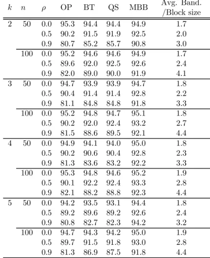
Table 1. Coverage Rates of Nominal 95% symmetric Percentile-t Intervals: Logita k n ρ OP BT QS MBB Avg. Band. /Block size 2 50 0.0 95.3 94.4 94.4 94.9 1.7 0.5 90.2 91.5 91.9 92.5 2.0 0.9 80.7 85.2 85.7 90.8 3.0 100 0.0 95.2 94.6 94.6 94.9 1.7 0.5 89.6 92.0 92.5 92.6 2.4 0.9 82.0 89.0 90.0 91.9 4.1 3 50 0.0 94.7 93.9 93.9 94.7 1.8 0.5 90.4 91.4 91.4 92.8 2.2 0.9 81.1 84.8 84.8 91.8 3.3 100 0.0 95.2 94.8 94.7 95.1 1.8 0.5 90.2 92.0 92.4 93.2 2.7 0.9 81.5 88.6 89.5 92.1 4.4 4 50 0.0 94.9 94.1 94.0 95.0 1.8 0.5 90.2 90.6 90.4 92.8 2.3 0.9 81.3 83.6 83.2 92.2 3.3 100 0.0 95.3 94.8 94.6 95.2 1.9 0.5 90.1 92.2 92.4 93.3 2.8 0.9 82.1 88.2 88.8 92.3 4.4 5 50 0.0 94.2 93.5 93.1 94.4 1.8 0.5 89.2 89.6 89.2 92.6 2.4 0.9 80.8 82.7 82.3 94.2 3.2 100 0.0 94.7 94.3 94.2 95.0 1.9 0.5 89.7 91.5 91.8 93.0 2.8 0.9 81.3 86.9 87.5 91.8 4.4 a_{10,000 Monte Carlo trials with 999 bootstrap replications each.}

The main results are: a) when ρ = 0 all methods work well, even for n = 50; b) when ρ 6= 0 all intervals undercover, but the robust methods (BT, QS and MBB) outperform OP, as expected. The undercoverage is worse the larger is k and the smaller is n (an exception is MBB when k = 5, ρ = 0.9, perhaps due to the larger rate of non-convergence); c) the MBB always outperforms BT or QS, especially for small n and large k, and d) the average bandwidth/block size is larger for larger ρ and n, as expected.

ConÞdence Intervals for ARCH models We assume the following DGP:

(4.1) yt= ¯γ + εt, εt= vth1/2t , ht= ¯ω + ¯αε2_t−1.

A bar denotes true parameters and a superscript o denotes pseudo-true parameters throughout. Usually {vt} is assumed i.i.d. Here, we generate vt as AR(1):

(4.2) vt= ¯ρvt−1+ ut, |¯ρ| < 1, ut∼ i.i.d. N ¡

0, σ2_u¢, σ2_{u = 1 − ¯ρ}2.

We can write (4.1)-(4.2) as yt = ¯γ + ¯ρh1/2t h−1/2t−1 (yt−1− ¯γ) + h1/2t ut, with ut ∼ i.i.d. N ¡

0, σ2_u¢. For ¯

ρ = 0, this is the usual ARCH(1). For ¯_{ρ 6= 0 an extra term appears. Letting F}t−1 = σ (. . . y_t−2, y_t−1) and using v_t−1= ε_t−1/h1/2_t−1, we have E¡ε_t|Ft−1¢= ¯ρh1/2_t v_t−1and E¡ε2_t|Ft−1¢= ht

¡

1 − ¯ρ2+ ¯ρ2v2_t−1¢, so E¡yt_|Ft−1¢= ¯γ +¯ρh1/2_t h_t−1−1/2(y_{t−1− ¯γ) and var}¡yt_|Ft−1¢= σ2_uht. We (mis)specify a Gaussian ARCH(1) model parameterized by θ = (γ, ω, α)0:

yt= γ + et, et|Ft−1∼ N (0, ht(θ)) , t = 1, . . . , n,

with ht(θ) = ω + αe2_t−1. The QMLE ˆθn maximizes the log-likelihood

(4.3) Ln(θ) = 1 2n

n X t=1

log ft(θ) , where log ft_{(θ) = −} µ ln ht(θ) + e 2 t ht(θ) ¶ .

The model is correctly speciÞed if and only if ¯ρ = 0. With misspeciÞcation the QMLE is generally inconsistent for ¯θ = (¯γ, ¯ω, ¯α) ; instead conÞdence intervals for pseudo-true parameters θo = (γo_{, ω}o_{, α}o₎ pertain. We evaluate θoby simulation, as the value maximizing the expectation of (4.3), computed using 50,000 simulations. Considering the expected score corresponding to γ, we have

(4.4) E¡s1t ¡_¯ θo¢¢= E µ αoε_t−1 ht(θo) − ε2_t h2 t(θo) (αoε_t−1) + εt ht(θo) ¶ = 0,

where ¯θo = (¯γ, ωo, αo)0, ht¡¯θo¢= ωo+ αoε2_t−1and εt= yt_{− ¯γ. For suitably symmetric joint distributions} of (εt, ε_t−1) centered at zero, it is plausible that this expectation equals zero, implying that γo = ¯γ, despite the misspeciÞcation. Proving this conjecture would distract us from our purpose here, but our simulations (with normal errors) always delivered γo = ¯γ. Accordingly we set γo= ¯γ in what follows.

With misspeciÞcation, the scores are generally not a martingale difference sequence, justifying the use of robust inference on θo. As before, we consider OP, BT, QS and MBB. All but OP are robust to

Table 2. Coverage Rates of Nominal 95% symmetric Percentile-t Intervals: ARCHa n α¯ ρ¯ C.I. for θ OP BT QS MBB Avg. Band.

/Block size 200 0.5 0.0 γ¯ 94.4 94.4 94.4 95.0 1.37 ¯ ω 93.6 93.5 93.6 95.4 ¯ α 91.8 91.5 91.4 94.9 0.5 γ¯ 83.8 90.9 91.7 93.0 4.50 ωo _{93.8 93.2 93.2 95.6} αo _{92.6 92.6 92.6 95.4} 0.9 γ¯ 60.3 76.0 77.0 86.4 6.49 ωo 91.6 91.9 91.9 95.7 αo _{82.4 92.4 93.0 94.6} 500 0.5 0.0 γ¯ 94.8 94.8 94.8 95.0 1.35 ¯ ω 94.5 94.6 94.6 95.5 ¯ α 93.6 93.5 93.4 94.7 0.5 γ¯ 85.0 92.6 93.0 93.5 6.11 ωo 94.9 94.3 94.3 95.4 αo 93.3 94.0 94.1 95.4 0.9 γ¯ 62.9 83.2 83.7 87.6 9.16 ωo 94.0 94.0 94.0 95.5 αo 80.0 93.5 94.1 94.7 200 0.9 0.0 γ¯ 94.5 94.4 94.4 95.1 1.34 ¯ ω 93.2 93.2 93.2 95.3 ¯ α 92.3 92.2 92.2 94.9 0.5 γ¯ 86.7 91.3 92.0 93.2 3.54 ωo 93.1 92.9 92.9 95.4 αo 92.0 93.0 93.2 95.4 0.9 γ¯ 65.1 77.0 78.0 88.3 5.39 ωo 90.3 90.6 90.6 95.4 αo 69.6 86.6 88.0 89.6 500 0.9 0.0 γ¯ 94.8 94.8 94.9 95.1 1.32 ¯ ω 94.3 94.3 94.3 95.4 ¯ α 93.4 93.4 93.4 94.3 0.5 γ¯ 88.0 92.6 93.0 93.5 4.82 ωo 94.4 94.0 94.0 95.2 αo 92.4 94.6 94.9 95.8 0.9 γ¯ 69.2 84.4 84.8 88.8 7.66 ωo 93.6 93.8 93.8 95.5 αo 68.7 90.4 91.1 92.2

a_{10,000 Monte Carlo trials with 999 bootstrap replications each. Pseudo-true parameters were calculated} by 50,000 simulations: forα = 0.5, (ω¯ o, αo) = (0.07, 0.798)when ¯ρ = 0.5 and(ωo, αo) = (0.017, 1.130) when¯ρ = 0.9; forα = 0.9, (ω¯ o_{, α}o_{) = (0.069, 1.192)when ¯ρ = 0.5 and (ω}o_{, α}o_{) = (0.015, 1.480)when ¯ρ = 0.9. γ = 1.0¯ and ω = 0.1¯} were set throughout.

misspeciÞcation. The OP interval is valid if the Þrst two conditional moments of yt are not misspeciÞed. Data on {yt} were generated by (4.1)-(4.2) with ¯γ = 1.0, ¯ω = 0.1 and six combinations of ¯α and ¯ρ taken from ¯_{α ∈ {0.5, 0.9} and ¯ρ ∈ {0.0, 0.5, 0.9}. Table 2 contains results. We summarize as follows.} When ¯ρ = 0 all methods tend to perform well, though the coverage of the BT and QS intervals tends

to slightly understate the true levels for ¯ω and ¯α. In contrast, the MBB intervals achieve almost correct coverage for ¯θ, with slight overstatement for ¯ω. When ¯ρ = 0, the scores are a martingale difference sequence, and this is reßected in the bandwidth/block size parameter. When ¯_{ρ 6= 0, major Þndings} are: (i) the OP intervals fail dramatically for ¯γ, exhibiting severe undercoverage which worsens as ¯ρ increases; (ii) the coverages of BT and QS for ¯γ are also well below the 95% nominal level, but we see clear improvement as n increases; (iii) the MBB outperforms the HAC methods; and (iv) the average chosen bandwidth/block size exceeds one, and tends to increase with n, as we expect.

5. Conclusion

The results presented here justify routine use of MBB methods for the QMLE in a general context. Further results in our setting establishing higher order improvements for the MBB (with recentering) are a logical next step and a promising subject for future work.

Appendix A: Assumptions and Proofs for Section 2

Throughout Appendix A, P is the probability measure governing the behavior of the original time series while P∗

n,ωdenotes the probability measure induced by the bootstrap. For any bootstrap statistic Tn∗(·, ω) we write T∗

n(·, ω) → 0 prob − Pn,ω, a.s. − P if for any ε > 0 there exists F ∈ F with P (F ) = 1 such that∗ for all ω in F, lim_n→∞P_n,ω∗ _{[λ : |Tn}∗_{(λ, ω)| > ε] = 0. We write Tn}∗_{(·, ω) → 0 prob−Pn,ω, prob −P if for any}∗ ε > 0 and for any δ > 0, lim_n→∞P£ω : P_n,ω∗ _{[λ : |Tn}∗_{(λ, ω)| > ε] > δ}¤= 0. Using a subsequence argument (e.g. Billingsley, 1995, Theorem 20.5), T_n∗_{(·, ω) → 0 prob − Pn,ω}∗ _{, prob − P is equivalent to having that} for any subsequence {n0} there exists a further subsequence {n00} such that Tn∗00(·, ω) → 0 prob − Pn∗00,ω, a.s. − P. For any distribution D we write Tn∗(·, ω) ⇒

dP ∗_n,ω

D prob − P when for every subsequence there exists a further subsequence for which weak convergence under P_n,ω∗ _{takes place almost surely −P .}

Assumption A is the doubly indexed counterpart of the regularity conditions used by GW. Assumption A

A.1: _{Let (Ω, F, P ) be a complete probability space. The observed data are a realization of a stochastic} process ©Xnt : Ω → Rl, l ∈ N, n, t ∈ N

ª

, with Xnt(ω) = Wnt(. . . , Vt−1(ω) , Vt(ω) , Vt+1(ω) , . . .) , Vt_{: Ω → R}v_{, v ∈ N, and W}nt: ×∞_{τ =−∞}Rv → Rl such that Xnt is measurable for all n, t.

A.2: The functions fnt : Rlt× Θ → R+ are such that fnt(·, θ) is measurable for each θ ∈ Θ, a compact subset of Rp, p ∈ N, and fnt¡X_{n, ·}t ¢_{: Θ → R}+ _{is continuous on Θ a.s. − P , n, t = 1, 2, . . . .}

A.5: (i)©log fnt ¡

Xt n, θ

¢ª

is Lipschitz continuous on Θ, i.e. ¯¯log fnt ¡ Xt n, θ ¢ − log fnt¡Xt n, θo¢¯¯ ≤ Lnt |θ − θo| a.s. − P , ∀θ, θo ∈ Θ, where supn©n−1Pn_t=1E (Lnt)

ª

= O (1) . (ii) ©_∇2log fnt ¡

X_nt, θ¢ª is Lipschitz continuous on Θ.

A.6: For some r > 2: (i)©log fnt ¡

X_nt, θ¢ª _{is r−dominated on Θ uniformly in n, t, i.e. there exists} Dnt : Rlt → R such that

¯

¯log fnt¡X_nt, θ¢¯¯ _{≤ Dnt} for all θ in Θ and Dnt is measurable such that kDntkr ≤ ∆ < ∞ for all n, t. (ii)

©

∇ log fnt ¡

X_nt, θ¢ª is r-dominated on Θ uniformly in n, t. (iii) ©

∇2log fnt¡X_nt, θ¢ªis r-dominated on Θ uniformly in n, t. A.7: _{Vt} is an α-mixing sequence of size −_r−22r , with r > 2. A.8: The elements of (i) ©log fnt

¡ Xt

n, θ ¢ª

are NED on {Vt} of size −12; (ii) ©

∇ log fnt¡Xt n, θ

¢ª are NED on {Vt} of size −1 uniformly on (Θ, ρ) , where ρ is any convenient norm on Rp_{, and (iii)} ©

∇2log fnt ¡

X_nt, θ¢ª_{are NED on {Vt} of size −}1₂ uniformly on (Θ, ρ) . A.9: (i) nB_no _{≡ var}³n−12 Pn

t=1∇ log fnt ¡

X_nt, θo_n¢´o is uniformly positive deÞnite. (ii) ©Ao_{n≡ E}¡n−1Pn_t=1∇2log fnt¡X_nt, θo_n¢¢ªis uniformly nonsingular.

The usefulness of the following lemmas extends beyond the QMLE as they apply to prove the validity of bootstrap methods for other extremum estimators, such as GMM.

Lemma A.1 (IdentiÞable uniqueness of ˆθn). Let (Ω, F, P ) be a complete probability space and let Θ be a compact subset of Rp_{, p ∈ N. Let} ©_Q

n: Ω × Θ → R ª

be a sequence of random functions continuous on Θ a.s. − P, and let ˆθn = arg maxΘQn(·, θ) a.s. − P . If sup_θ∈Θ

¯

¯Qn(·, θ) − Qn(θ) ¯ ¯ → 0 a.s.-P and if ©Q_{n: Θ → R}ª _{has identiÞably unique maximizers {θ}o_{n} on Θ, then} nˆθn

o

is identiÞably unique on Θ with respect to {Qn} a.s. − P, i.e. there exists F ∈ F, P (F ) = 1, such that given any ε > 0 and some δ (ε) > 0, for each ω ∈ F, there exists N (ω, ε) < ∞ such that

sup n≥N(ω,ε) " max ηc₍ˆ_θn,ε)Qn(ω, θ) − Qn ³ ω, ˆθn ´# ≤ −δ (ε) < 0, where ηc_n ³ ˆ θn, ε ´

is the compact complement of η ³ ˆ θn, ε ´ ≡ n θ ∈ Θ : ¯ ¯ ¯θ − ˆθn ¯ ¯ ¯ < εo. If instead sup_θ∈Θ¯¯Qn(·, θ) − Qn(θ) ¯

¯ → 0 prob − P then for any subsequencenˆ_θn0o_ofnˆ_θno_{, there exists a further} subsequence nˆθn00

o

such thatnˆθn00 o

is identiÞably unique with respect to {Qn00} a.s. − P .

Lemma A.2 (Consistency of ˆθ∗_n). _{Let (Ω, F, P ) be a complete probability space and let Θ be a} com-pact subset of Rp_{, p ∈ N. Let}©_Q

n: Ω × Θ → R ª

be such that (a1) Qn(·, θ) : Ω → R is measurable-F for each θ ∈ Θ; (a2) Qn(ω, ·) : Θ → R is continuous on Θ a.s. − P . Let ˆθn = arg maxΘQn(., θ) a.s. − P be measurable and assume there exists©Q_{n: Θ → R}ª_{with identiÞably unique maximizers {θ}o_{n} such that} (a3) sup_θ∈Θ¯¯Qn(·, θ) − Qn(θ)

¯

(A) ˆθn− θon→ 0 prob − P.

Let (Λ, G) be a measurable space, and for each ω ∈ Ω and n ∈ N let ¡Λ, G, Pn,ω∗ ¢

be a complete probability space. Let ©Q∗_{n: Λ × Ω × Θ → R}ª be such that (b1) Q∗_{n(·, ω, θ) : Λ → R is measurable-G} for each (ω, θ) in Ω × Θ; (b2) Q∗n(λ, ω, ·) : Θ → R is continuous on Θ a.s. − P (i.e. for all λ and almost all ω). Let nˆθ∗_{n: Λ × Ω → Θ}o _{be such that for each ω ∈ Ω, ˆθ}∗_{n(·, ω) : Λ → Θ is measurable-G and} ˆ

θ∗_{n(·, ω) = arg maxΘ}Q∗_{n(·, ω, θ) a.s. − P . Assume further that (b3) supθ∈Θ|Q}∗_{n(·, ω, θ) − Q}n(ω, θ)| → 0 prob − Pn,ω, prob − P . Then,∗

(B) ˆθ∗_{n(·, ω) − ˆθ}n(ω) → 0, prob − Pn,ω∗ , prob − P.

Lemma A.3 (Asymptotic Normality of ˆθ∗_n). Let (Ω, F, P ) be a complete probability space and let Θ be a compact subset of Rp_{, p ∈ N. Let} ©_Q

n: Ω × Θ → R ª

be such that (a1) Qn(·, θ) : Ω → R is measurable-F for each θ ∈ Θ; (a2) Qn(ω, ·) : Θ → R is continuously differentiable of order 2 on Θ a.s. − P . Let ˆθn= arg maxΘQn(·, θ) a.s. − P be measurable such that ˆθn− θon→ 0 prob − P, where {θon} is interior to Θ uniformly in n. Suppose there exists a nonstochastic sequence of p × p matrices {Bn}o that is O (1) and uniformly positive deÞnite such that (a3) Bno−1/2√n∇Qn(·, θon) ⇒ N (0, Ip). Suppose further that there exists a sequence {An: Θ → Rp×p} such that {An} is continuous on Θ uniformly in n, and (a4) sup_θ∈Θ¯¯∇2Qn_{(·, θ) − A}n(θ)

¯ ¯ → 0 prob − P, where {Ao n≡ An(θon)} is O (1) and uniformly nonsingular. Then (A) B_no−1/2Ao_n√n ³ ˆ θn_{− θ}o_n ´ ⇒ N (0, Ip) .

Let (Λ, G) be a measurable space, and for each ω ∈ Ω and n ∈ N, let ¡Λ, G, P∗ n,ω

¢

be a complete probability space. Let ©Q∗

n: Λ × Ω × Θ → R ª

be such that (b1) Q∗

n(·, ω, θ) : Λ → R is measurable-G for each (ω, θ) in Ω × Θ; (b2) Q∗

n(λ, ω, ·) : Θ → R is continuously differentiable of order 2 on Θ a.s. − P . For each n = 1, 2, . . . , let ˆθ∗n(·, ω) = arg maxΘQ∗n(·, ω, θ) a.s. − P be measurable such that ˆ

θ∗_{n(·, ω)−ˆθn(ω) → 0, prob−Pn,ω, prob−P. Assume further that (b3) B}∗ no−1/2√n∇Q∗n ³

·, ω, ˆθn(ω)´_⇒dP ∗_n,ω N (0, I_{p) in prob − P ; (b4) supθ∈Θ}¯¯∇2Q∗_{n(·, ω, θ) − ∇}2Qn(ω, θ)

¯

¯ → 0 prob − P_{n,ω, prob − P . Then}∗ (B) Bo−1/2_n Ao_n√n³θˆ∗_{n(·, ω) − ˆθn}(ω)´_⇒dP ∗_{n,ω N (0, I}

p) prob − P.

Lemma A.4 (Bootstrap Uniform WLLN). _{Let {q}∗_{nt(·, ω, θ)} be a MBB resample of {q}nt(ω, θ)} and assume: (a) For each θ ∈ Θ ⊂ Rp, Θ a compact set, n−1Pn_t=1(q∗_{nt(·, ω, θ) − q}nt(ω, θ)) → 0, prob − P_{n,ω, prob − P ; and (b) ∀θ, θ}∗ o _{∈ Θ, |q}nt(·, θ) − qnt(·, θo)| ≤ Lnt|θ − θo| a.s. − P, where

sup_n©n−1Pn

t=1E (Lnt) ª

= O (1) . Then, if `n= o (n) , for any δ > 0 and ξ > 0, lim n→∞P " P_n,ω∗ Ã sup θ∈Θ n−1 ¯ ¯ ¯ ¯ ¯ n X t=1 (q_nt∗ _{(·, ω, θ) − qnt}(ω, θ)) ¯ ¯ ¯ ¯ ¯> δ ! > ξ # = 0.

Lemma A.5 (Bootstrap Pointwise WLLN). _{For some r > 2, let {qnt : Ω × Θ → R} be such that} for all n, t, there exists Dnt: Ω → R with |qnt(·, θ)| ≤ Dnt for all θ ∈ Θ and kDntkr≤ ∆ < ∞. For each θ ∈ Θ let {qnt∗ (·, ω, θ)} be a MBB resample of {qnt(ω, θ)}. If `n = o (n) , then for any δ > 0, ξ > 0, and for each θ ∈ Θ, lim n→∞P " P_n,ω∗ Ã n−1 ¯ ¯ ¯ ¯ ¯ n X t=1 (q_nt∗ _{(·, ω, θ) − q}nt(ω, θ)) ¯ ¯ ¯ ¯ ¯> δ ! > ξ # = 0.

Lemma A.6. _{Let {Qn: Ω × Θ → R} be a sequence of functions continuous on Θ a.s. − P and let} n

ˆ

θn: Ω → Θ o

be such that ˆθn− θon → 0 prob − P . Suppose supθ∈Θ ¯

¯Qn(·, θ) − Qn(θ) ¯

¯ → 0 prob − P where ©Q_{n: Θ → R}ªis continuous on Θ uniformly in n. Then,

(A) Qn

³

·, ˆθn(·)´− Qn(θo_{n) → 0 prob − P.} For each ω ∈ Ω, let ¡Λ, G, Pn,ω∗

¢

be a complete probability space. If ˆθ∗_{n(·, ω) − ˆθn(ω) → 0 prob − Pω,n}∗ , prob − P and supθ∈Θ|Q∗n(·, ω, θ) − Qn(ω, θ)| → 0 prob − Pn,ω, prob − P, then∗

(B) Q∗_n³_{·, ω, ˆθ}∗_{n(·, ω)}´_{− Q}n ³

ω, ˆθn(ω)´_{→ 0 prob − Pn,ω}∗ _{, prob − P.}

Proof of Theorem 2.1. We apply Lemma A.2 with Qn(·, θ) = n−1Pnt=1qnt(·, θ) and Q∗n(·, ω, θ) = n−1Pn t=1q∗nt(·, ω, θ) , where qnt(·, θ) ≡ log fnt ¡ Xt n(·) , θ ¢ , and {q∗

nt(·, ω, θ)} is the MBB resample. Con-ditions (a1)-(a3) are readily veriÞed under Assumption A. Assumption A.2. implies (b1) and (b2). To verify (b3) apply Lemmas A.4 and A.5, noting that `n = o (n). ¥

Proof of Theorem 2.2. We apply Lemma A.3 with the same choices of Qn(·, θ) and Q∗n(·, ω, θ) as in Theorem 2.1. The result follows then by Polya’s theorem (e.g. Serßing, 1980, p. 20) since C_no = Ao−1_n B_noAo−1_n is O (1) and the normal distribution is everywhere continuous. (a1)-(a4) can be veriÞed as in Theorem 5.7 of GW. (b1) and (b2) follow from A.2. Lemmas A.4 and A.5 imply (b4) given A.5(ii) and A.6(iii) and the conditions on `n. Lastly, we verify (b3). We have that (for any n and any ω)

n−1/2 n X t=1 s∗_nt³_{·, ω, ˆθn}´_{− n}−1/2 n X t=1 snt ³ ω, ˆθn ´ = ξ_1n+ ξ_2n+ ξ_3n, where ξ_{1n(·, ω) ≡ n}−1/2Pn_t=1(s∗_{nt(·, ω, θ}o_{n) − s}nt(ω, θon)) ; ξ2n(ω) ≡ −n−1/2 Pn t=1 ³ snt ³ ω, ˆθn ´ − snt(ω, θon) ´ ; and ξ_{3n(·, ω) ≡ n}−1/2Pn_t=1 ³ s∗_nt ³ ·, ω, ˆθn ´ − s∗nt(·, ω, θon) ´

. It suffices to show that for any subsequence n0 there exists a further subsequence n00 _{such that a.s. − P (i) Bn}o−1/200 ξ1n00(·, ω) ⇒

dP ∗

n00,ω _{N (0, I}

p), and (ii) ξ_2n00(ω) + ξ3n00(·, ω) → 0 prob − P_n∗00,ω. The result then follows by Lemma 4.7 of White (2000), since n00−1Pn_t=100 sn00t

³ ω, ˆθn00

´

= 0 for all n00 _{sufficiently large, a.s. − P , by A.3(ii) and the F.O.C. for ˆθ}n00. Theorem 2.2 of Gonçalves and White (2001) implies (i) under Assumption A strengthened by 2.1 and 2.2. To prove (ii), let F ≡ F1∩ F2, with F1 the set of ω on which (i) holds, and F2 the set on which the remaining conditions of Lemma A.3 hold. Note that P (F ) = 1. For Þxed ω in F, two mean value expansions yield

ξ_2n00(ω) + ξ3n00(·, ω) = ζn00(·, ω) √ n00³ˆ_{θn00(ω) − θ}o n00 ´ , ζ_n00(·, ω) = n 00₋₁Pn00 t=1 ¡ ∇0s∗ n00_t ¡ ·, ω, ¯θ∗n00 ¢ − ∇0sn00t ¡

ω, ¯θn00¢¢, with ¯θn00 and ¯θ∗_n00 (possibly different) mean values lying between ˆθn00 and θo_n00. Lemma A.6 implies ζn00(·, ω) → 0 prob − P_n∗00_,ω for all ω ∈ F , given the uniform convergence of ©_∇2Q∗_n00(·, ω, θ) − ∇2Qn00(ω, θ)ª and ©∇2Qn00(ω, θ) − An00(θ)ª, and the convergences of ¯θn00− θo_n00 and ¯θ∗n00− θo_n00 to zero. Since

√

n00³ˆ_{θn00(ω) − θ}o n00

´

= O (1) on F , it follows that ξ_2n00(ω) + ξ3n00(·, ω) → 0 prob − P_n∗00,ω for ω ∈ F , P (F ) = 1. ¥

Proof of Corollary 2.1. We can show√n³ˆθ∗_{1n− ˆθ}n ´

−√n³ˆθ∗_{n− ˆθ}n ´

→ 0 prob − Pn,ω∗ , prob − P , given the deÞnition of ˆθ∗_1n and the fact that ˆA∗_{n− ˆ}An_{→ 0 prob − Pn,ω, prob − P, by Lemma A.6. ¥}∗

Proof of Lemma A.1. _{Let F ≡} n ω : ˆθn_{(ω) − θ}o_{n→ 0} o ∩©ω : sup_Θ¯¯Qn(ω, θ) − Qn(θ) ¯ ¯ → 0ª. By The-orem 3.4 of White (1994), P (F ) = 1. Fix ε0 _{> 0 and ω in F . Then, there exists N0(ω, ε}0_{) < ∞ such that} for all n > N0(ω, ε0) , ¯ ¯ ¯ˆθn(ω) − θon ¯ ¯ ¯ < ε0_{. Because {θ}o

n} is identiÞably unique on Θ, given ε0 _{> 0 there} ex-ists N1(ε0) < ∞ and δ0(ε0) > 0 such that sup_n≥N1(ε0)

£ max_ηc_(θo n,ε0)Qn(θ) − Qn(θ o n) ¤ ≡ −δ0(ε0) < 0, where η (θo_n, ε0_{) ≡ {θ ∈ Θ : |θ − θ}o_{n| < ε}0_{}. By Corollary 3.8 of White (1994), there exists N2}¡ω, δ0(ε0)¢ _{< ∞} such that for all n > N2

¡ ω, δ0(ε0)¢, ¯ ¯ ¯Qn ³ ω, ˆθn(ω) ´ − Qn(θo_n) ¯ ¯

¯ < δ0(ε40). Also, for all n > N2 ¡ ω, δ0(ε0)¢, maxηc_(θo n,ε0)Qn(ω, θ) ≤ maxηc(θon,ε0)Qn(θ)+ δ0_(ε0₎ 4 . Let N (ω, ε0) = max © N0(ω, ε0) , N1(ε0) , N2 ¡ ω, δ0(ε0)¢ª. Hence sup n≥N(ω,ε0) " max ηc(ˆ_{θn(ω),2ε0)}Qn(ω, θ) − Qn ³ ω, ˆθn(ω)´ # ≤ sup n≥N(ω,ε0) · max ηc(θo_n,ε0)Qn(ω, θ) − Qn(θ o n) + δ0(ε0) 4 ¸ ≤ sup n≥N (ω,ε0₎ · max ηc_(θo n,ε0) Q_{n(θ) − Qn}(θo_n) +2δ 0_(ε0₎ 4 ¸ ≤ −δ 0_(ε0₎ 2 .

Set ε = 2ε0 and δ (ε) = δ0(ε/2)₂ > 0 to obtain the result for all ω in F and P (F ) = 1. If instead sup_Θ¯¯Qn(ω, θ) − Qn(θ)

¯

¯ → 0 prob − P, then for any {n0_{} there exists {n}00_{} such that} sup_Θ¯¯Qn00(ω, θ) − Qn00(θ)

¯

¯ = o (1) and ˆθn00(ω) − θo_n00 = o (1) a.s. − P . The result thus holds for {n00} a.s. − P . ¥

Proof of Lemma A.2. (A) follows by Theorem 3.4 of White (1994) under (a1)-(a3). To prove (B), note that for any subsequence {n0}, by Lemma A.1 there exists {n00} such that

n ˆ θn00

o

is identiÞably unique a.s. − P , given (a1)-(a3). Now apply Theorem 3.4 of White (1994). ¥

Proof of Lemma A.3. (A) follows by White’s (1994) Theorem 6.2 under (a1)-(a4). To prove (B), it suffices to show that for any subsequence {n0} there exists a further subsequence {n00} such that B∗−1/2_n00 A∗_n00

√

n00³ˆ_θ∗_{n00(·, ω) − ˆθn00(ω)}´ _⇒dP ∗n00,ω _{N (0, Ip) , a.s. − P . This follows by applying White’s} (1994) Theorem 6.2 to an appropriately chosen subsequence, given ω in F such that P (F) = 1. ¥ Proof of Lemma A.4. The proof closely follows that of Lemma 8 of Hall and Horowitz (1996).

Proof of Lemma A.5. _{Fix θ ∈ Θ, and write n}−1Pn t=1(qnt∗ (θ) − qnt(θ)) = Q1n+ Q2n, with Q1n≡ n−1 n X t=1 (q_nt∗ _{(θ) − E}∗(q_nt∗ (θ))) , and Q2n≡ E∗ Ã n−1 n X t=1 q∗_nt(θ) ! − n−1 n X t=1 qnt(θ) ,

where we omit ω to conserve space. Q2n _{→ 0 prob − P since E}∗¡n−1Pn_t=1q∗_nt(θ)¢= n−1Pn_t=1qnt(θ) + OP¡_n`¢(cf. Lemma A.1 of Fitzenberger (1997)) and <sub>n</sub>` _{→ 0. By Chebyshev’s inequality, for any δ > 0,} P∗ n,ω(|Q1n| > δ) ≤ _δ12n−1var∗ ¡ n−1/2Pn t=1q∗nt(θ) ¢ , where var∗¡_n−1/2Pn t=1q∗nt(θ) ¢

has a closed form expression involving products of qnt(θ) and qn,t+τ (θ) (cf. Gonçalves and White (2001)). Under the domination condition on {qnt(θ)} and the properties of the MBB, repeated application of Minkowski and Hölder’s inequalities yields°°var∗¡n−1/2Pn_t=1q_nt∗ (θ)¢°°r

2

= O (`) for some r > 2. Thus, by Markov’s inequality, P£P_n,ω∗ _(|Q1n| > δ) > ξ¤= O

³¡_` n

¢r/2´

→ 0 given ` = o (n). ¥

Proof of Lemma A.6. (A) holds by White (1994, Corollary 3.8). (B) By uniform continuity of ¯Qn on Θ, given ε > 0 there exists δ (ε) > 0 such that ¯¯_{¯ ¯}Qn(θ) − ¯Qn

³ ˆ θn´¯¯¯ > ε/3 implies ¯ ¯ ¯θ − ˆθn ¯ ¯ ¯ > δ (ε) . So P h P_n,ω∗ ³¯¯_¯Q∗_n ³ ·, ω, ˆθ∗n ´ − Qn ³ ω, ˆθn´¯¯_{¯ > ε} ´ > ε i ≤ P · P_n,ω∗ µ sup Θ |Q ∗ n(·, ω, θ) − Qn(ω, θ)| > ε/3 ¶ > ε/3 ¸ +P · P_n,ω∗ µ 2 sup Θ ¯ ¯Qn(ω, θ) − ¯Qn(θ) ¯ ¯ > ε/3¶> ε/3 ¸ + PhP_n,ω∗ ³¯¯_¯ˆθ∗_{n− ˆθn} ¯ ¯ ¯ > δ (ε)´> ε/3i_{≡ ξ1}+ ξ₂+ ξ₃, with obvious deÞnitions. By uniform convergence of Q∗_{n(·, ω, θ) − Qn}(ω, θ) to zero, ξ_{1 → 0. Similarly, by} uniform convergence of Qn_{(·, θ)− ¯}Qn(θ) to zero, ξ_{2→ 0 since ξ2≤ P}¡2 sup_Θ¯¯Qn(ω, θ) − ¯Qn(θ)

¯

¯ > ε/3¢. Finally, ξ_{3 → 0 because ˆθ}∗_{n(·, ω) − ˆθ}n(ω) → 0 prob − Pn,ω, prob − P. ¥∗

Appendix B: Proofs for Section 3

Throughout Appendix B, C denotes a generic constant. The dependence of the bootstrap variables on ω and on n will also be omitted as it is not relevant for the arguments made here.

Lemma B.1 (Studentization of the sample mean). _{Let {Xnt} satisfy Assumptions 2.1}0 and 2.2 of Gonçalves and White (2001), where Assumption 2.20 is strengthened by

A.2.20 n−1Pn_{t=1|µnt− ¯}µ_n|2+δ = o ³

`−1−δ/2n ´

for some δ such that 0 < δ ≤ 2. Then, if `n→ ∞ with `n= o

¡

n1/2¢we have that for any ε > 0, lim_n→∞P¡P∗¡¯¯ˆσ∗2_{n − ˆ}σ2_n¯¯ > ε¢ > ε¢ = 0, where ˆσ2_n= var∗¡√n ¯X_n∗¢and ˆσ∗2_n = k−1Pk_i=1³`−1/2P`_t=1¡XIi+t− ¯Xn∗

¢´2 .

Lemma B.2. _{Let {X}nt} and {Znt} satisfy kXntk2+δ ≤ ∆ and kZntk2+δ ≤ ∆, t = 1, . . . , n, n = 1, 2, . . . , for any 0 < δ ≤ 2 and some ∆ < ∞. Let k = n/`. If {Ii}ki=1 are i.i.d. uniform on {0, . . . , n − `} and if `n→ ∞ and `n= o

¡

n1/2¢_{, then for any ε > 0,}

lim n→∞P à P∗ﯯ_¯ ¯k−1 k X i=1 `−1 ` X t=1 Xn,Ii+t ` X t=1 Zn,Ii+t ¯ ¯ ¯ ¯ ¯> n 1/2_ε ! > ε ! = 0.

Proof of Theorem 3.1_{. By GW’s Theorem 7.5 Wn ⇒ X}2

q under Ho. Next, we prove Wn∗ ⇒dP ∗ Xq2 prob − P . A mean value expansion of rn

³ ˆ θ∗_n´ around ˆθn yields √n ³ rn ³ ˆ θ∗_n´_{− rn}³ˆθn ´´ ⇒dP ∗ N (0, Ro_nC_noR_no0_{) prob−P, implying n (ˆ}r∗_{n− ˆrn})0(R_noC_noRo0_n)−1(ˆr_n∗_{− ˆrn) ⇒}dP ∗ _X2

q prob−P. Thus, it suffices to prove: (i) ˆR∗_{n− R}o_{n → 0 prob − P}∗_{, prob − P ; (ii) ˆ}A∗_{n− A}o_{n → 0 prob − P}∗_{, prob − P ; and (iii)}

ˆ

B∗_{n− Bn}o _{→ 0 prob − P}∗_{, prob − P. (i) follows by continuity of rn} on Θ (uniformly in n) and because ˆ

θ∗_{n− θ}o_{n → 0 prob − P}∗_{, prob − P by Theorem 2.1; similarly, by Theorem 2.1 and Lemma A.6, we have} ˆ

A∗_{n− ˆ}An_{→ 0 prob − P}∗_{, prob − P , which implies (ii) since ˆ}An_{− A}o_{n→ 0 prob − P . To prove (iii), consider} ˜ B_n∗o = k−1 k X i=1 Ã `−1/2 ` X t=1 ¡ sn,Ii+t ¡ XIi+t n , θon ¢ − ¯s∗on ¢! Ã `−1/2 ` X t=1 ¡ sn,Ii+t ¡ XIi+t n , θon ¢ − ¯s∗on ¢!0 = k−1 k X i=1 `−1 ` X t=1 sn,Ii+t ¡ XIi+t n , θon ¢X` t=1 s0<sub>n,I</sub> i+t ¡ XIi+t n , θon ¢ − `¯s∗ons¯∗o0n , (B.1)

where ¯s∗o_n = n−1Pn_t=1s∗_nt(θ_no) . By Lemma B.1 ˜B_n∗o _{− Bn,1}o _{→ 0, prob − P}∗_{, prob − P , where Bn,1}o = var∗¡n−1/2Pn_t=1s∗_nt(θo_n)¢. By Gonçalves and White’s (2001) Corollary 2.1, B_n,1o _{− Bn}o _{→ 0, prob − P ,} implying ˜B_n∗o_{− Bn}o _{→ 0, prob − P}∗_{, prob − P . Thus, it suffices that ˆ}B_n∗_{− ˜}B_n∗o _{→ 0, prob − P}∗_{, prob − P .} From (3.1) and (B.1) we can write ˆB_n∗_{− ˜}B_n∗o= D1+ D2, where

D1 ≡ k−1 k X i=1 `−1 " <sub>`</sub> X t=1 sn,Ii+t ³ XIi+t n , ˆθ ∗ n ´_X` t=1 s0<sub>n,Ii+t</sub>³XIi+t n , ˆθ ∗ n ´ − ` X t=1 sn,Ii+t ¡ XIi+t n , θon ¢X` t=1 s0_n,Ii+t¡XIi+t n , θon ¢#

and D2 _{≡ `¯s}∗o_n¯s∗o0_n . Note that ¯s∗o_n = Bno1/2Bno−1/2(¯s∗on − ¯son) + B o1/2

n Bno−1/2s¯on ≡ E1 + E2, with ¯son = n−1Pn_t=1so_nt. We have E1= OP∗¡n−1/2¢prob − P by Gonçalves and White’s (2001) Theorem 2.2, and E2 = OP

¡

n−1/2¢ _{by the CLT for {s}o_{nt}. Thus, D2 → 0 prob − P}∗_{, prob − P. To show that D1 → 0} prob − P∗_{, prob − P we take a mean value expansion about θ}o

n of a typical element of D1 and apply Lemma B.2 twice with Xnt= sup_θ∈Θ

¯ ¯ ∂ ∂θ0snt,j ¡ X_nt, θ¢¯¯and Znt = sup_θ∈Θ ¯ ¯snt,j ¡ X_nt, θ¢¯¯. ¥

Proof of Theorem 3.2. The proof follows GW (Theorem 7.9, p. 128) using Lemmas B.1 and B.2. Proof of Lemma B.1. The proof consists of two steps: (1) show ˜σ∗2_{n − ˆ}σ2_{n → 0 prob − P}∗_{, prob − P,} where ˜σ∗2_n = k−1Pk_i=1³`−1/2P`_t=1¡XIi+t− ¯Xα,n

¢´2

, with ¯Xα,n = E∗ ¡_¯

X_n∗¢; (2) show ˆσ∗2_{n − ˜σ}∗2_{n → 0} prob − P∗, prob − P. Let ˆAi = `−1/2P`_t=1¡Xi+t_{− ¯}X_n∗¢ and Ai = `−1/2P`_t=1¡Xi+t_{− ¯}Xα,n¢ so that ˆ σ∗2_n = k−1Pk_i=1Aˆ2_I i and ˜σ ∗2 n,1= k−1 Pk

i=1A2Ii. (1) By two applications of Markov’s inequality it suffices to show E¡E∗¯¯˜σ∗2

n − ˆσ2n ¯

¯p¢ _{= o (1) for some p > 1. We take p = 1 + δ/2 with 0 < δ ≤ 2. Since} E∗¡_˜σ∗2 n ¢ = E∗¡_A2 I1 ¢

= (n − ` + 1)−1Pn−`i=0A2i ≡ ˆσ2n(cf. Künsch (1989, Theorems 3.1 and 3.4)), we have E∗¯¯˜σ∗2_{n − ˆ}σ2_n¯¯p = E∗ ¯ ¯ ¯ ¯ ¯k−1 k X i=1 ¡ A2_{Ii− E}∗¡A2_I1¢¢ ¯ ¯ ¯ ¯ ¯ p ≤ k−pCE∗ ¯ ¯ ¯ ¯ ¯ k X i=1 ¡ A2_{Ii− E}∗¡A2_I1¢¢2 ¯ ¯ ¯ ¯ ¯ p/2 ,

by Burkholder’s inequality, because©A2 Ii− E

∗¡_A2 I1

¢ª

are (conditionally) i.i.d. zero mean. For 1 < p ≤ 2, x ≥ 0 and y ≥ 0, the inequality (x + y)p/2 ≤ xp/2+ yp/2 implies E∗

¯ ¯ ¯Pki=1 ¡ A2_I i− E ∗¡_A2 I1 ¢¢2¯_¯ ¯p/2 ≤ kE∗¯¯A2_I 1 − E ∗¡_A2 I1¢¯¯ p

so that E∗¯¯˜σ∗2_{n − ˆ}σ2_n¯¯p _{≤ 2}pCk−(p−1)E∗_|AI1|2p. Thus, it suffices that k−(p−1)E³E∗_|AI1|2p´= o (1) . Some algebra yields E³E∗_|AI1|2p´_{≤ C (F1}+ F2+ F3), where

F1 = (n − ` + 1)−1 n−` X i=0 `−pE   ¯ ¯ ¯ ¯ ¯ ` X t=1 Zn,i+t ¯ ¯ ¯ ¯ ¯ 2p  ; F2 = (n − ` + 1)−1 n−` X i=0 `−p ¯ ¯ ¯ ¯ ¯ ` X t=1 ¡ µ_{n,i+t− ¯}µ_α,n¢ ¯ ¯ ¯ ¯ ¯ 2p , and F3 = (n − ` + 1)−1Pn−`_i=0`−pE ³¯<sub>¯` ¯</sub> Zα,n ¯ ¯2p´

, with Znt ≡ Xnt − µnt, and for any {Ynt} ¯Yα,n = (n − ` + 1)−1Pn−`i=0`−1

P`

t=1Yn,i+t = Pn

t=1αntYnt with αnt = _(n−`+1)`1 min {t, `, n − t + 1}. Under As-sumption 2.10, E ¯ ¯ ¯P`t=1Zn,i+t ¯ ¯

¯2p< C`p (cf. Gonçalves and White (2001), p.18 for a similar argument), implying k−(p−1)<sub>F1 = O</sub>³¡`

n

¢p−1´ _{= o (1), and similarly for k−(p−1)F}

3. If µnt = µ for all t, F2 = 0 because ¯µ_α,n =Pn_t=1αntµ = µ as Pnt=1αnt = 1. Otherwise, by A.2.20, F2 = o (1), so k−(p−1)F2 = o (1). For (2), note ˆAIi = √ `¡X¯Ii− ¯Xn∗ ¢ , where ¯XIi = `−1 P` t=1XIi+t, and Ai = √ `¡X¯Ii− ¯Xα,n ¢ , implying ˆ σ∗2_{n − ˜}σ∗2<sub>n = −`</sub>¡X¯<sub>n</sub>∗<sub>− ¯</sub>Xα,n ¢2 = OP∗¡<sub>n</sub>`¢→ 0 prob − P , since √n¡X¯_n∗− ¯Xα,n ¢ ⇒dP ∗ _{N (0, 1) prob − P} by Theorem 2.2 of Gonçalves and White (2001). ¥

Proof of Lemma B.2. Let S_n,i1 = P`<sub>t=1</sub>Xn,i+t and Sn,i2 = P`

t=1Zn,i+t.By Markov’s inequality, for some 1 < p ≤ 2, it suffices to show n−p/2E∗³¯¯_¯k−1Pk_i=1`−1S_n,I1

iS 2 n,Ii ¯ ¯ ¯p´→ 0 prob − P . Let p = 1 + δ/2, 0 < δ ≤ 2, and note E∗³¯¯¯k−1Pk i=1`−1Sn,I1 iS 2 n,Ii ¯ ¯ ¯p´≤ C (F1+ F2), with F1= E∗ﯯ_¯ ¯k−1 k X i=1

`−1¡S<sub>n,I</sub>1 <sub>i</sub>S<sub>n,I</sub>2 <sub>i− E</sub>∗¡S<sub>n,I</sub>1 <sub>i</sub>S<sub>n,I</sub>2 <sub>i</sub>¢¢ ¯ ¯ ¯ ¯ ¯ p! and F2 = E∗ ¯ ¯ ¯ ¯ ¯k−1 k X i=1 `−1E∗¡S_n,I1 _iS_n,I2 _i¢ ¯ ¯ ¯ ¯ ¯ p .

By the Burkholder and cr-inequalities F1 <sub>≤ C`</sub>−pk−(p−1)E∗ ¯ ¯ ¯S1 n,I1S 2 n,I1 ¯ ¯ ¯p ≤ C`−pE∗ ¯ ¯ ¯S1 n,I1S 2 n,I1 ¯ ¯ ¯p, since n S_n,I1 iS 2 n,Ii− E ∗³_S1 n,IiS 2 n,Ii ´o

are i.i.d. zero mean, and k−(p−1) _{≤ 1 for p > 1. Similarly, F}2 ≤ C`−p_E∗¯¯_¯S1 n,I1S 2 n,I1 ¯ ¯

¯p. By the Cauchy-Schwarz and Minkowski inequalities, E³E∗¯¯_¯S1 n,I1S 2 n,I1 ¯ ¯ ¯p´≤ C`2p<sub>.</sub> Thus, F1+ F2 = OP(`p), and so n−p/2(F1+ F2)P = O ³³ ` n1/2 ´p´ = op(1) , since ` = o ¡ n1/2¢_. ¥

References

[1] Andrews, D.W.K. (1991): “Heteroskedasticity and Autocorrelation Consistent Covariance Matrix Estimation,” Econometrica, 59, 817-858.

[2] (2001): “Higher-order Improvements of a Computationally Attractive k-step Bootstrap,” Econometrica, 69, forthcoming.

[3] Billingsley, P. (1995): Probability and Measure, New York: Wiley.

[4] Corradi, V., and N. R. Swanson (2001): “Bootstrap Conditional Distribution Tests under Dynamic MisspeciÞcation,” University of Exeter, manuscript.

[5] Davison, A.C., and P. Hall (1993): “On Studentizing and Blocking Methods for Implementing the Bootstrap with Dependent Data,” Australian Journal of Statistics, 35, 215-224.

[7] Davidson, R., and J.G. MacKinnon (1999): “Bootstrap Testing in Nonlinear Models,” Inter-national Economic Review, 40, 487-508.

[8] Fitzenberger, B. (1997): “The Moving Blocks Bootstrap and Robust Inference for Linear Least Squares and Quantile Regressions,” Journal of Econometrics, 82, 235-287.

[9] Gallant, A.R., and H. White (1988): A UniÞed Theory of Estimation and Inference for Non-linear Dynamic Models. New York: Basil Blackwell.

[10] Ghosh, M., W.C. Parr, W.C., K. Singh, and G.J. Babu (1984): “A Note on Bootstrapping the Sample Median,” Annals of Statistics, 12, 1130-1135.

[11] GONÇALVES, S., and H. White (2001): “The Bootstrap of the Mean for Dependent Heteroge-neous Arrays,” forthcoming Econometric Theory.

[12] (2000): “Bootstrap Variance Estimation for Smooth Functions of Sample Means and for Linear Regressions,” Université de Montréal, manuscript.

[13] GÖTZE, F., and H.R. KÜNSCH(1996): “Second-order Correctness of the Blockwise Bootstrap for Stationary Observations,” Annals of Statistics, 24, 1914-1933.

[14] Gourieroux, C., Monfort, A. and A. Trognon (1984), “Estimation and Test in Probit Models with Serial Correlation,” in Alternative Approaches to Time Series Analysis, ed. Florens, J.P., Mouchart, M., Raoult, J.P. and L. Simar. Brussels: Publications des Facultés Universitaires Saint-Louis.

[15] Hahn, J. (1996): “A Note on Bootstrapping Generalized Method of Moments Estimators,” Econo-metric Theory, 12, 187-197.

[16] Hall, P., and J. Horowitz (1996): “Bootstrap Critical Values for Tests based on Generalized-Method-of-Moments Estimators,” Econometrica, 64, 891-916.

[17] Inoue, A. and Shintani, M. (2001) “Bootstrapping GMM estimators for Time Series,” North Carolina State University, manuscript.

[18] KÜNSCH, H.R. (1989): “The Jackknife and the Bootstrap for General Stationary Observations,” Annals of Statistics, 17, 1217-1241.

[19] Lahiri, S.N. (1996): “On Edgeworth Expansion and Moving Block Bootstrap for Studentized M-Estimators in Multiple Linear Regression Models,” Journal of Multivariate Analysis, 56, 42-59. [20] Liu, R.Y., and K. Singh (1992) “Moving Blocks Jackknife and Bootstrap Capture Weak

De-pendence,” in Exploring the Limits of the Bootstrap, ed. by R. LePage and L. Billiard. New York: Wiley.

[21] Newey, W.K., and K.D. West (1987): “A Simple Positive Semi-deÞnite, Heteroskedastic and Autocorrelation Consistent Covariance Matrix,” Econometrica, 55, 703-708.

[22] Politis, D., and J. Romano (1992): “A General Resampling Scheme for Triangular Arrays of α-mixing Random Variables with Application to the Problem of Spectral Density Estimation,” Annals of Statistics, 20, 1985-2007.

[23] PÖTSCHER, B.M., and I.R. Prucha (1991): “Basic Structure of the Asymptotic Theory in Dy-namic Nonlinear Econometric Models, Part I: Consistency and Approximation Concepts,” Econo-metric Reviews, 10, 125-216.

[24] Serfling, R.J. (1980): Approximation Theorems of Mathematical Statistics. New York: Wiley. [25] Shao, J. (1992): “Bootstrap Variance Estimators with Truncation,” Statistics and Probability

Letters, 15, 95-101.

[26] White, H. (1994): Estimation, Inference and SpeciÞcation Analysis. Cambridge: Cambridge Uni-versity Press.

Liste des publications au CIRANO*

Série Scientifique / Scientific Series (ISSN 1198-8177)

2002s-41

Maximum Likelihood and the Bootstrap for Nonlinear Dynamic Models / Sílvia

Gonçalves, Halbert White

2002s-40

Selective Penalization Of Polluters: An Inf-Convolution Approach / Ngo Van

Long et Antoine Soubeyran

2002s-39

On the Mediational Role of Feelings of Self-Determination in the Workplace:

Further Evidence and Generalization / Marc R. Blais et Nathalie M. Brière

2002s-38

The Interaction Between Global Task Motivation and the Motivational Function

of Events on Self-Regulation: Is Sauce for the Goose, Sauce for the Gander? /

Marc R. Blais et Ursula Hess

2002s-37

Static Versus Dynamic Structural Models of Depression: The Case of the CES-D /

Andrea S. Riddle, Marc R. Blais et Ursula Hess

2002s-36

A Multi-Group Investigation of the CES-D's Measurement Structure Across

Adolescents, Young Adults and Middle-Aged Adults / Andrea S. Riddle, Marc R.

Blais et Ursula Hess

2002s-35

Comparative Advantage, Learning, and Sectoral Wage Determination / Robert

Gibbons, Lawrence F. Katz, Thomas Lemieux et Daniel Parent

2002s-34

European Economic Integration and the Labour Compact, 1850-1913 / Michael

Huberman et Wayne Lewchuk

2002s-33

Which Volatility Model for Option Valuation? / Peter Christoffersen et Kris Jacobs

2002s-32

Production Technology, Information Technology, and Vertical Integration under

Asymmetric Information / Gamal Atallah

2002s-31

Dynamique Motivationnelle de l’Épuisement et du Bien-être chez des Enseignants

Africains / Manon Levesque, Marc R. Blais, Ursula Hess

2002s-30

Motivation, Comportements Organisationnels Discrétionnaires et Bien-être en Milieu

Africain : Quand le Devoir Oblige / Manon Levesque, Marc R. Blais et Ursula Hess

2002s-29

Tax Incentives and Fertility in Canada: Permanent vs. Transitory Effects / Daniel

Parent et Ling Wang

2002s-28

The Causal Effect of High School Employment on Educational Attainment in Canada

/ Daniel Parent

2002s-27

Employer-Supported Training in Canada and Its Impact on Mobility and Wages

/ Daniel Parent

2002s-26

Restructuring and Economic Performance: The Experience of the Tunisian Economy

/ Sofiane Ghali and Pierre Mohnen

2002s-25

What Type of Enterprise Forges Close Links With Universities and Government

Labs? Evidence From CIS 2 / Pierre Mohnen et Cathy Hoareau

* Consultez la liste complète des publications du CIRANO et les publications elles-mêmes sur notre site Internet :