COMPARISON BETWEEN MULTITEMPORAL GRAPH BASED CLASSICAL LEARNING AND LSTM MODEL CLASSIFICATIONS FOR SITS ANALYSIS

HAL Id: hal-02954635

https://hal.telecom-paris.fr/hal-02954635

Submitted on 1 Oct 2020

HAL is a multi-disciplinary open access

archive for the deposit and dissemination of

sci-entific research documents, whether they are

pub-lished or not. The documents may come from

teaching and research institutions in France or

abroad, or from public or private research centers.

L’archive ouverte pluridisciplinaire HAL, est

destinée au dépôt et à la diffusion de documents

scientifiques de niveau recherche, publiés ou non,

émanant des établissements d’enseignement et de

recherche français ou étrangers, des laboratoires

publics ou privés.

COMPARISON BETWEEN MULTITEMPORAL

GRAPH BASED CLASSICAL LEARNING AND

LSTM MODEL CLASSIFICATIONS FOR SITS

ANALYSIS

Ferdaous Chaabane, Safa Réjichi, Florence Tupin

To cite this version:

Ferdaous Chaabane, Safa Réjichi, Florence Tupin. COMPARISON BETWEEN MULTITEMPORAL

GRAPH BASED CLASSICAL LEARNING AND LSTM MODEL CLASSIFICATIONS FOR SITS

ANALYSIS. IGARSS (International Conference on Geoscience and Remote Sensing), Sep 2020, Hawaï,

United States. �hal-02954635�

COMPARISON BETWEEN MULTITEMPORAL GRAPH BASED CLASSICAL LEARNING

AND LSTM MODEL CLASSIFICATIONS FOR SITS ANALYSIS

Ferdaous Chaabane

_{, Safa Réjichi}

_{, Florence Tupin}

(1) COSIM laboratory, SUP’COM, Carthage University, Tunisia

(2) Department of Image and Signal Processing, Telecom ParisTech, France

ABSTRACT

Very High Resolution (VHR) multispectral Satellite Image Time Series (SITS) enables the production of temporal land cover maps, thanks to high spatial, temporal and spectral resolution of modern earth observation programs.

Besides, statistical learning methods applied to SITS monitoring and analysis have created relatively efficient semi-automatic classification techniques. It would therefore be natural to think that the use of deep learning methods on SITS would lead to advances comparable to those known in the field of computer vision. However, when applied to concrete cases, the results are not as convincing. This paper proposes a comparison between a SOTAG (Spatial-Object Temporal Adjacency Graphs) SVM based spatio-temporal classification approach and the Recurrent Neuronal Network (RNN), LSTM (Long Short-Term Memory) model which is trained by historical SITS. The trained LSTM networks are then used to predict new time series data. Both methods perform a spatio-temporal map indicating the temporal profiles of cartographic regions. The proposed approaches will be applied on real and simulated SITS data. We will demonstrate that both results are comparable despite computational times and algorithms complexity.

Index Terms— SITS analysis, temporal profiles

classification, Graph based SVM classification, RNN, LSTM model, etc.

1. INTRODUCTION

Recently, the analysis of multitemporal remote sensing data has interested researchers who use such information to construct SITS and perform change detection, monitor geographical zones, apply dynamic monitoring of natural phenology, etc. The question is: How competently monitoring and analyzing SITS is a real challenge in remote sensing field?

In the context of land cover monitoring using multitemporal classification techniques, we aims to distinguish among different temporal profiles classes.

Several works directly apply standard machine learning approaches ( Random Forest (RF), Support Vector Machine (SVM), etc.) either on the pixel or the region level [1] [2]. Especially, researchers focused their attention on supervised techniques for the classification and monitoring of different types of Remote Sensing images acquired by new generation satellite sensors

More recently, in [3], the authors examined and compared the performances of the RF, KNN, and SVM classifiers for land cover classification using Sentinel-2 image data. In [4], an original expert knowledge-based SITS analysis technique for land-cover monitoring and region dynamics assessing has been proposed. Region temporal profiles similar to a given scenario proposed by the user are extracted, which can be useful in many applications such as urbanization and forest regions’ monitoring.

Besides, the deep learning revolution proved that neural network models are adapted tools to manage and automatically classify SITS data, while standard convolutional neural networks’ (CNNs) techniques [5] are well suited to deal with spatial autocorrelation, the same approaches are sometimes not adapted to correctly manage long and complex temporal evolutions. Researchers started then to compare NN techniques to classical learning ones [6]. They demonstrate that ANN achieved the highest OA followed by SVM and RF. However, analysis of the stability of results concluded that RF and SVM had the lowest variance of OA. Only few studies exist involving temporal deep learning approaches (i.e. RNNs) to deal with remote sensing time series. In [7], the ability of RNNs, in particular, the LSTM model, to perform land cover classification considering SITS is evaluated. An extensive research has been conducted on modeling temporal dynamics by spectro-temporal profiles using vegetation indices in [8]. The authors proposed a deep learning approach to utilize these temporal characteristics for classification tasks. They show how long LSTM model can be employed for crop identification purposes with SITS Sentinel 2A observations. The paper presents a comparison of two temporal classification algorithms belonging to classical and deep learning families. The aim of this work is to evaluate both approaches in an attempt to classify the temporal evolution of cartographic areas starting from SITS data. We focus

mainly on the classification of groups of spatially adjacent pixels with homogenous temporal evolution over the SITS. The SVM based technique proposed in a previous work [9] build a graph for each region of the first SITS classified image characterizing its temporal evolution when using discriminative signatures for vertices and edges labelling. Then, a MGK SVM based algorithm is used to analyse and classify the obtained graphs. The resulted temporal map discerns between the land cover classes behaviours (stable, expanded, etc.).

The second deep learning method uses the LSTM networks which can store theoretically unlimited amount of evidence and make decisions in actual temporal context. In this work, we propose to use LSTM networks for the purpose of cartographic regions temporal profiles classification. Pixels temporal profiles extracted from the STIS data are used to train the model and perform a temporal classification map. The analysis of SITS classification is then evaluated by comparing the performance of deep learning temporal LSTM models and the Graph SVM based model.

This paper is organized as follows. The second section presents the main steps of the graph based classical learning approach. Then, the LSTM temporal technique is detailed in the third section. Finally, simulated and real data description and experimental results are highlighted and discussed in the fourth section.

2. CLASSICAL LEARNING SVM GRAPH BASED APPROACH

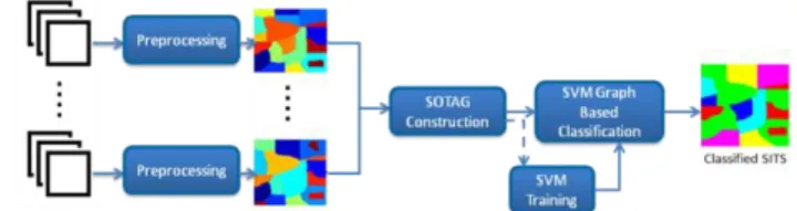
This section presents a summary of the proposed multitemporal SITS classification principle detailed in [9] (cf. Figure1). As illustrated, we first need to identify the spatio-temporal regions included in the SITS by applying classification on each image. SITS images are supposed to be pretreated (pansharpening and co-registration) before applying classification.

Figure 1. Cartographic regions monitoring using temporal graphs classification.

Then, spatially homogenous regions are temporally analyzed through graph construction. Indeed, a SOTAG is constructed for each region of the first image. Here, we use chronological order to arrange SITS images. The SOTAG begins by a region of the first image and it grows up involving following SITS images. In those graphs, a node represents a region and an edge represents the temporal relationship between regions. The nodes are labelled using discriminative signatures. For spectral signature, we use

obviously radiometric values and specified indices such as: the Normalized Difference Vegetation Index (NDVI) which is used to discriminate vegetation regions; The Soil Brightness Index (SBI) which is used to characterize bare soil; The Difference Water Index (NDWI) and the Index Surfaces Built (ISU) which are intended respectively for water and urban areas. For textural signature, the mean, the standard deviation, the entropy, the energy and Gabor wavelet decomposition features are used to identify texture variation.

However, the edges are labelled according to area intersection (neighborhood overlap) between temporal regions as images are co-registered. After SOTAGs construction, they are all classified using a graph kernel SVM based algorithm (cf. Figure1). This step is done in order to extract regions with similar temporal evolutions. In this paper, we use a particular graph-based kernel called Marginalized Graph Kernel, introduced by Kashima et al. [4]. It uses the concept of random walk which is a sequence of labels and vertices selected on a graph along a random path. The adapted expression and all the mathematical framework of this MGK is detailed in [4]. It allows the spatio-temporal classification of the SITS basing on graph forms.

3. DEEP LEARNING LSTM BASED CLASSIFICATION

RNNs are well known deep learning techniques that demonstrate their efficiency in different domains and especially in remote sensing field. Unlike CNNs, RNNs manage temporal data dependences, since the output of the neuron at time t -1 is used, together with the next input, to feed the neuron itself at time t.

Figure 2. Network structure of the LSTM based classifier used for SITS temporal classification.

As mentioned in the introduction the most well-known type of RNN is the LSTM model. The LSTM model used in this paper is mainly introduced to learn temporal-term pixels variations. We used the LSTM unit described in [8]. The input of the LSTM is a sequence of variables where a generic element is the radiometric intensity of a pixel which refers to a corresponding timestamp.

3.1. Sample augmentation for classification

More samples are needed to train a deep learning model (such as LSTM) than that to train traditional machine learning algorithms (in our case SVM). However, in practice, there are limited field-survey samples, and collecting a volume of field samples would be very time consuming. This constitutes a major disadvantage of deep learning algorithms used in remote sensing applications. In our experiments, a limited number of field-survey samples are insufficient for training the deep learning model. Thus, pixels within a parcel were used for sample augmentation to enhance the stability and generalization of the classifier.

3.2. LSTM model for classification

For our framework we used Keras to build and train the LSTM model. In this LSTM network (as shown in Figure2), the multiple normalized (using the minmax normalization method with the minimum and maximum values from all time-series curves of the corresponding radiometries) time-series curves of samples were taken as the input, and the output temporal profiles types were encoded via one-hot encoding, a common technique to categorical classification in machine learning. Then, four LSTM layers with 36 hidden neurons (this is the optimal value in this study) were stacked to transfer raw time-series curves into high-level features. Then, a dense layer was employed to fully connect the high-level features to temporal profiles categories. Finally, a Softmax activation function output the probabilities of temporal types to produce a temporal classification maps.

4. RESULTS

First, the proposed SITS classification approaches are applied on simulated data with predefined regions. Here, we aim to quantitatively evaluate both techniques independently from the spatial segmentation and the pixels artifacts which may introduce some errors. Then, qualitative evaluation is established for a real SITS. Six temporal classes, have been defined according to feature families in order to monitor the covered area : Stable; progressive appearance; progressive disappearance; periodic change; abrupt change and random behavior.

4.1. Validation on Synthesized SITS data

4.1.1. Synthesized SITS generation

In order to evaluate the two proposed SITS classification approaches accuracy, we simulate a SITS composed of 15 images, using different information extracted from real ones. The synthesized images size is 300300 pixels composed of 4 spectral bands (Red, Blue, Green and Near-Infrared bands). To preserve ground components radiometry and texture as represented in a remote-sensing image, we used a simple non-parametric texture synthesis algorithm [10].

Figure 3. Synthesized multispectral SITS images samples (3 of 15 images in false color).

4.1.2. Comparison results

As the ground truth map is available for synthesized SITS, classification accuracy is given for simulated data by means of Overall Accuracy (OA) and Kappa index. We address in this section the comparison between the improved classical learning SVM based technique and the deep learning LSTM model which is the main contribution of this paper. The experimental results show that the graph-based approach achieves an OA of 88.64% and a Kappa of 0.81 compared with 86.91% and 0.75 for the LSTM based one. This result is illustrated by figure 4 where we can see comparable results. the effect of the low-level (pixel level) analysis for LSTM is revealed by some misclassified pixels. According to the same figure, we notice that the graph-based approach succeed to recognize 15 regions among 18 ones and the LSTM based one 14 regions among 18.

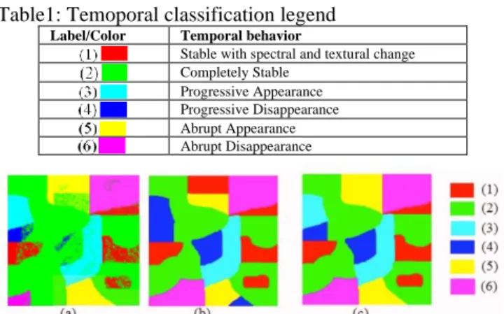
Table1: Temoporal classification legend

Label/Color Temporal behavior

Stable with spectral and textural change Completely Stable

Progressive Appearance Progressive Disappearance Abrupt Appearance Abrupt Disappearance

Figure 4. Synthesized SITS classification results: LSTM-based approach (a), SVM Graph-LSTM-based approach (b) and ground truth (c). Classes are presented in Table1.

This comparable results can be explained by the fact that features used to classify the regions are more discriminating than using only pixels temporal profiles. But due to computational time of LSTM training phase the graph based approach is more preferable.

4.2. Validation on Real SITS Data

For real SITS, we use as mentioned five images: one IKONOS image acquired on February 6, 2001 and four QUICKBIRD images acquired, respectively, on April 20, 2002, September 11, 2004, June 21, 2005, and June 27,

Figure 5. 5 VHR images of the SITS covering different types of changes. 2010 covering Zaghouan region in Tunisia. Figure5 shows

the 5 images of the SITS. The selected region shows different temporal behaviors as new buildings construction and roads extension. The forest region which is dominant is more or less stable.

Figure 6. (a) SVM Graph-based approach classification result; (b) LSTM based approach classification result. Classes are presented in Table1.

The LSTM based result has been post-treated using morphological tools (Label by label) to eliminate isolated pixels and small connected components. As we can notice from Figure6, the LSTM-based approach is focusing on small changes as it is pixel based. But it succeed to better extract the construction zone limits and the new road extension (purple color). It is also sensitive to spectral and textural changes present in forest regions (green instead of red color for small regions). However, the forest regions globally stable (red color) and the bared soil regions stable with spectral changes (green color) are better delimited using the SVM Graph-based approach.

As both approaches have different good and bad classification situations, the qualitative observation shows that they are globally comparable.

5. CONCLUSION

This works addressed the temporal classification of VHR SITS using two different approaches. The first one is SVM Graph based machine learning algorithm and the second one used the LSTM deep learning well known technique. The obtained classification results have different aspects as the first approach focuses on a global spatial evolution (region based) and the second one is independent from the spatial distribution as it uses the temporal evolutions of pixels. The qualitative results are also comparable and don’t boost any approach over the other. However, the second method is more consuming and need many samples for training. To conclude, we may suggest the

choice of the appropriate technique according to the nature of regions and the consumption time. A fusion of both approaches can be considered for a future work.

6. REFERENCES

[1] G. Mountrakis, J. C. Ogole, “Support vector machines in remote sensing: A review,” ISPRS Journal of Photogrammetry and

Remote Sensing, 66(33), pp 247-259, May 2011.

[2] L. Bruzzone, B. Demir, “A Review of Modern Approaches to Classification of Remote Sensing Data,” Land Use and Land Cover Mapping in Europe pp 127-143, Springer, January 2014.

[3] P. T. Noi, M. Kappas Comparison of Random Forest, k-Nearest Neighbor, and Support Vector Machine Classifiers for Land Cover Classification Using Sentinel-2 Imagery, Sensors 2018.

[4] S. Rejichi, F. Chaabane, F. Tupin, “Expert knowledge-based method for Satellite Image Time Series analysis and interpretation,” IEEE Journal of Selected Topics in Applied Earth

Observations and Remote Sensing (J-STARS), vol. 8, no. 5, pp.

2138-2150, May 2015. and Remote Sensing (J-STARS), vol. 8, no. 5, pp. 2138-2150, May 2015.

[5] S. Paul; V. Poliyapram; D. N. Kumar; R. Nakamura, “Performance evaluation of convolutional neural network at hyperspectral and multispectral resolution for classification,” SPIE

Remote Sensing, (11155), Strasbourg, France 2019.

[6] E. Raczko, B. Zagajewski, “Comparison of support vector machine, random forest and neural network classifiers for tree species classification on airborne hyperspectral APEX images,” European Journal of Remote Sensing, 50(1) pp 144-154 09 Mar 2017.

[7] Dino Ienco ; Raffaele Gaetano ; Claire Dupaquier ; , “Land Cover Classification via Multitemporal Spatial Data by Deep Recurrent Neural Networks,” IEEE Geoscience and Remote

Sensing Letters, (14)10, October 2017.

[8] M. Rußwurm, M. Körner, “MULTI-TEMPORAL LAND COVER CLASSIFICATION WITH LONG SHORT-TERMMEMORY NEURAL NETWORKS,” The International

Archives of the Photogrammetry, Remote Sensing and Spatial Information Sciences, Hannover, 6–9 June 2017.

[9] S. Rejichi and F. Chaabane, “Satellite Image Time Series Classification and Analysis using an Adapted Graph Labeling,” 8th MULTITEMP, pp.55-58, Annecy, France, 22-24 July 2015. [10] R.A. Fisher, “The use of Multiple Measurements in Taxonomic Problems,” Ann.Eugen., vol. 7, pp. 179-188, 1936.