Measuring mortality heterogeneity with multi-state models and interval-censored data

(1)

HAL Id: hal-01215350

https://hal.archives-ouvertes.fr/hal-01215350

Preprint submitted on 14 Oct 2015

HAL is a multi-disciplinary open access

archive for the deposit and dissemination of sci-entific research documents, whether they are pub-lished or not. The documents may come from teaching and research institutions in France or abroad, or from public or private research centers.

L’archive ouverte pluridisciplinaire HAL, est destinée au dépôt et à la diffusion de documents scientifiques de niveau recherche, publiés ou non, émanant des établissements d’enseignement et de recherche français ou étrangers, des laboratoires publics ou privés.

Measuring mortality heterogeneity with multi-state

models and interval-censored data

Alexandre Boumezoued, Nicole El Karoui, Stéphane Loisel

To cite this version:

Alexandre Boumezoued, Nicole El Karoui, Stéphane Loisel. Measuring mortality heterogeneity with multi-state models and interval-censored data. 2015. �hal-01215350�

(2)

Measuring mortality heterogeneity with

multi-state models and interval-censored data

1 Alexandre Boumezoued

2

, Nicole El Karoui

2

, Stéphane Loisel

3

October 14, 2015

Abstract

In this paper, our aim is to measure mortality rates which are specific to individual observable factors when these can change during life. The study is based on longitudinal data recording marital status and socio-professional features at census times, therefore the observation scheme is interval-censored since individual characteristics are only observed at isolated dates and transition times remain unknown. To this aim, we develop a parametric maximum likelihood estimation procedure for multi-state models that takes into account both interval-censoring and reversible transitions. This method, inspired by recent ad-vances in the statistical literature, allows us to capture characteristic-specific mortality rates, in particular to recover the mortality compensation law at high ages, but also to capture the age pattern of characteristics changes. The dynamics of several population compositions is addressed, and allows us to give explanations on the pattern of aggregate mortality, as well as on the impact on typical life insurance products. Particular attention is devoted to characteristics changes and parameter uncertainty that are both crucial to take into account.

Keywords: Mortality heterogeneity, longevity risk, multi-state models, interval-censoring, parametric maximum likelihood.

1_{This work benefited from the financial support of the ANR project Lolita (ANR-13-BS01-0011).}

2_{Laboratoire de Probabilités et Modèles Aléatoires (LPMA), UMR CNRS 7599}

Université Paris 6, 4 Place Jussieu, 75005 Paris, France. Email: alexandre.boumezoued@upmc.fr

Email: nicole.el_karoui@upmc.fr

3_{Institut de Science Financière et d’Assurances (ISFA), Université de Lyon,}

Université Claude Bernard Lyon 1, 50 Avenue Tony Garnier, F-69007 Lyon, France Email: stephane.loisel@univ-lyon1.fr

(3)

1 Introduction

Mortality at the individual level is known to depend on several observable factors, among the first ones age and gender. At a deeper level, one can have access to datasets recording other observable characteristics, such as socio-economic features or marital status. In this context, to capture mortality differentials depending on several characteristics is a key issue to better assess longevity/mortality risk at sev-eral levels. This paper is indeed motivated by reserving purposes regarding specific insurance portfolios, but also by a population dynamics point of view. This point of view, detailed in Bensusan et al. (2010-2015), allows to better understand how aggregate mortality and other demographic quantities as the age pyramid evolve with an underlying dynamic heterogeneity, based on populations evolving due to characteristic-specific mortality rates but also birth rates, as well as characteristics changes during life (see also Boumezoued (2015)).

From a statistical point of view, in the case where these characteristics are stable during life, classical survival analysis can be used to measure characteristic-specific mortality rates. However, when these characteristics can change over time, the model to be used is a multi-state model: a given individual switches from a state to another until death, which is an absorbing state. The first advantage of such model is to capture the characteristic-specific mortality rates but also the transition intensities from a characteristic to another. This provides a measure of the level of each possible transition in the model. Another advantage of such approach concerns parameter uncertainty: as the whole dynamics is captured, this approach provides the variance of the transition rates, as well as their correlations. This way, it is possible to take into account estimation error in the life trajectories of a given group of individuals.

To study life trajectories embedding characteristics changes, it is not possible to use the classical survival analysis estimators as Kaplan-Meier for the survival curve or Nelson-Aalen for the cumulative intensity. Indeed, such estimators will suffer from several statistical biases when applied to life trajectories with several inter-mediate states, since for example the user will proceed to an arbitrary distribution of individuals by mode, set once for all, or because the terminal event (death in most cases) is treated as independent censoring (see e.g. Joly et al. (2002)). The statistical estimation of continuously observed multi-state models, involving clas-sical censoring and truncation, can be performed by the standard non-parametric estimator of Aalen-Johansen (see Aalen and Johansen (1978) and the book of An-dersen et al. (1993)). Although the Aalen-Johansen estimator, as a generalization of the Nelson-Aalen estimator in a multi-state framework, can be used with several kinds of incomplete observations, its use requires to know the exact transition dates. However in practice, the multi-state process is most often observed at some isolated

(4)

times: indeed, in so-called longitudinal data related to medical visits or times of census, the state of the individual (marital status, social class, ...) is known at in-spection dates only. Even if this gives some information, the transition times remain unknown: such observation scheme is called interval censoring. Note also that times of death are often exactly recorded, so that in fact the observation scheme is mixed: interval-censored intermediate states and exactly know absorbing state. Several de-mographic and actuarial studies in this field tackle this issue by limiting the scope to a discrete-time model, or making assumptions about the transition times in each interval.

In the demographic and actuarial literature, one can find several studies focusing on the statistical estimation of multi-state models in discrete time, or continuous time with exactly known transition times. Many of them focus on health insur-ance and Long Term Care (LTC). Gaüzère et al. (1999) estimate what is called an irreversible illness-death process, a process with states 1=healthy, 2=illness and 3=death, where only transitions 1→2, 1→3 and 2→3 are allowed. Gaüzère et al. (1999) assume that transitions occur at the middle of the censoring interval, there-fore uses the classical non-parametric framework of Aalen-Johansen since transition times are given by data modification. Czado and Rudolph (2002) estimates the transition intensities of multi-state model with Cox-proportional hazard model with known transition times, whereas Helms et al. (2005) proposes to directly compute the estimated transition probabilities by means of Aalen-Johansen estimator in this context. Also, Levantesi and Menzietti (2012) focus on a discrete-time irreversible illness-death model to study how transition probabilities change over time and mea-sure the so-called systematic risk. Apart from specific LTC and health insurance issues, the study of mortality differentials in general life insurance has also gained recent attention for a better understanding of national mortality and a better assess-ment of longevity/mortality risk. For example, Kwon and Jones (2006) and Kwon and Jones (2008) calibrate a discrete-time multi-state model from Canadian health longitudinal data (Canadian National Population Health Survey), and study the impact of mortality differentials on typical life and health insurance mechanisms.

To our knowledge, no actuarial studies focused on the assessment of mortality differentials in the presence of interval censoring, despite this is the main characteris-tic of longitudinal data. In this context, our aim is to capture mortality differentials with continuous age by means of reversible multi-state models when the data is interval-censored. We first develop a parametric maximum likelihood estimation procedure, which is inspired by recent advances in the statistical literature, and sec-ond apply it to a representative sample of the French national population made by the French institute INSEE, called Échantillon Démographique Permanent1

(5)

In the statistical literature, several contributions focused on multi-state model estimation with interval-censored data. On the whole, they can be classified de-pending on the type of method (parametric, semi-parametric, non-parametric), the class of multi-state models considered (illness-death reversible or not, competing risk, general multi-state) and the Markov assumption (Markov, semi-Markov, non-Markov). Since the seminal work of Kalbfleisch and Lawless (1985) in the case of constant intensities, methods have been developed for irreversible illness-death Markov models. In this context, one can find non-parametric approaches in e.g. Frydman (1995) and Frydman and Szarek (2009), and both semi-parametric and parametric methods in e.g. Joly et al. (2002), Commenges and Gégout-Petit (2007) and Commenges et al. (2007) (see also Foucher et al. (2007) and Touraine (2013)). As for reversible processes, one can find in the literature methods dedicated to spe-cial cases of multi-state models and intensities, as Kang and Lagakos (2007) and Titman and Sharples (2010) (see also Wei (2015)). Kang and Lagakos (2007) fo-cused on maximum likelihood estimation for homogenous semi-Markov multi-state models, assuming that at least one transition intensity is constant. Titman and Sharples (2010) developed an alternative method based on phase-type waiting times and hidden Markov chain models. Recently, Wei (2015) introduced a method based on quasi-Monte Carlo methods applied to time-independent semi-Markov models.

The advantage of non-parametric methods is to overcome assumptions about the shape of the transition intensities, which is also the case to some extent for semi-parametric methods as smooth basis functions remain unspecified. This is par-ticularly useful for applications for which we have no idea of the age structure of these intensities. Unfortunately, in the case of small samples and/or high number of interval-censored transition times, non-parametric methods may be unstable: the use of parametric methods then captures, for such kind of data, a maximum amount of information on the dynamics (see e.g. Foucher et al. (2007)). Let us emphasize that for several statistical studies, it is more reasonable to implement a parametric method taking into account interval censoring, rather than using a nonparametric method assuming that transition times are known (see e.g. Touraine et al. (2013)). Indeed, modifying the data by setting middle-interval transition times (or even uni-formly distributed) leads to fix the age pattern of the transition intensities between groups: to have intensities with jumps at fixed points for middle-interval assump-tion, or to be constant on the interval for uniformly simulated transition times. In this context, parametric methods allows to capture the age pattern of transition rates while avoiding several biases due to data modification. Parametric methods are also relevant to include information that we have on the shape of the mortality rates, for example a Gompertz-type mortality rate at reasonable ages. In this

(6)

text, and given the sample we want to study, we propose here a parametric approach that will allow us to include a maximum of a priori information on the shape of the intensity and reduce at best the dimension of the problem.

In the current statistical literature, parametric maximum likelihood procedures have not been developed for interval-censored data, when intensities depend on age or time, concerning Markov multi-state models which can have reversible transitions. So first, closely to e.g. Joly et al. (2002), Commenges et al. (2007), Foucher et al. (2007) and Touraine et al. (2013) who focus on irreversible processes, we develop such method. Second, we apply it to the French representative sample Échantil-lon Démographique Permanent to capture mortality forces which depend on socio-economic features or marital status, as well as transition intensities between the several groups. Special attention is given to parameter uncertainty, which can be different depending on the socio-economic group and the transition rate considered. This way, we are able to analyze the age-pattern of aggregate mortality which de-pends on the underlying sub-populations dynamics, as well as the impact on typical insurance products of heterogeneity and the associated level and uncertainty.

The remainder of this paper is organized as follows. In Section 2, we describe the longitudinal data we use as a basis for our estimation procedure. The para-metric maximum likelihood method that takes into account interval-censoring and reversible transitions in the multi-state model is detailed in Section 3, and the results we obtain are described in Section 4. Finally, in Section 5 we study the age pattern of aggregate mortality and we analyze the impact of heterogeneity on typical life insurance products.

2 Longitudinal data

In this section, we describe the data we want to analyze, which makes the statistical method developed in the next section conditional upon it. The Permanent De-mographic Sample (Échantillon Démographique Permanent) of the French institute INSEE is a longitudinal dataset which aims at observing a representative sample of the national population while recording several individual characteristics over time. It contains information of about 992,711 individuals observed since 1968 and born from 1862, the 1, 2, 3 or 4 of October. These individuals have been (potentially) observed at the census dates 1968, 1975, 1982, 1990 and 1999, and for each cen-sus, a set of characteristics was recorded: we here have access to socio-professional categories as well as marital status. Such a sample is useful to study the link be-tween the level of mortality and individual characteristics, but also the way these characteristics change over time.

(7)

Scope of the study This part of the Permanent Demographic Sample that we have access to is a remarkable database, especially given its completeness, its focus on real cohorts and regarding the set of characteristics involved. Also, the detailed analysis of specific levels of mortality in sub-populations and changes in their char-acteristics during life is a statistical task that poses two major constraints:

a) The size of the subpopulations considered has to be sufficient, which will guide us first to regroup several modalities of the classification of INSEE, and second to include one type of characteristics (socio-professional category or marital status) at a time.

b) The observation of the life trajectories must be sufficiently repeated over time, which will push us to consider specific cohorts making the five censuses (1968, 1975, 1982, 1990, 1999) available and exploitable given the characteristic considered.

Finally, note that the interval-censoring mechanism involved here has the par-ticularity to be common to all individuals. Therefore the age at which a given individual is observed depends on his/her date of birth. We are here in the case of dependent interval-censoring which is a statistical framework that is beyond the scope of the present paper. Therefore, we focus on specific cohorts and taking into account several cohorts at a time is left for further research. In the following, we detail the dataset we are interested in regarding the socio-professional groups as well as marital status.

Socio-professional categories For each year of census, (1968, 1975, 1982, 1990 and 1999), we have access to the socio-professional category of each observed indi-vidual. It is classified by the INSEE in a detailed way, therefore we choose to split them in two groups. The group 1 includes farmers, craftsmen, salesmen, low-skilled workers and people without work. The group 2 includes directors of 10 employees or more, managers, higher intellectual professions, middle management and employees. This classification, although arbitrary, will be useful to illustrate our methodology as well as to give interesting insights on the mortality differentials that are of inter-est for insurance purposes. In this study, we first focus on the male population of the 1930 birth cohort, which is the first to present a negligible number of students in 1968, which makes all times of census exploitable with the multi-state model described in Figure 1. This leads to a sample of 4266 individuals alive at the first census, observed or not. Group 1 of the 1930 birth cohort represents about 70 % of the population in 1968, and group 2 its complementary 30 %. In Figure 2, we represent the proportion of group 1 at each census. Over time, the composition of the cohort evolves according to two effects: first due to the fact that mortality for each group may be different, second due to characteristics changes during the

(8)

lifetime of individuals2_.

Marital status As well, we focus on marital status. Since we want to explore the impact of this characteristic at highest ages, we focus on the 1907 female birth cohort leading to observe individuals with age 60 at the first census. This leads to a sample of 3038 individuals alive at the first census, observed or not. The focus on marital status leads us to consider two groups. The first characteristic label regroups "single", "divorced" or "widowed", and the second characteristic label is "married". This choice is driven by the data which would not have been sufficient if we wanted to analyze transitions between "non-married" sub-groups. Although we lose some information on the original dataset, we are able to analyze the impact of being married or not, and the transitions between both, all of them being crucial for insurance purposes. The multi-state dynamics therefore considered is depicted in Figure 1. In Figure 3, we represent the proportion of non-married individuals at each census. As well, recall that the cohort composition evolves first due to the fact that mortality for each group may be different, and second due to characteristics changes during the lifetime of individuals.

With these two possible classifications, we want to illustrate two facts: hetero-geneity implies different mortality levels, and also different orders of magnitude of uncertainty around these levels. By the study of the dynamics of life trajectories within a cohort, it is possible to get further insights on the age pattern of aggregate mortality. We also want to illustrate that this is crucial to take into account char-acteristics changes during life, in particular when computing the price of typical life insurance products. Note that we estimate mortality forces by age for a real cohort, which contrasts with many actuarial studies that compute transition probabilities based on a mix of all age classes at a given year, therefore does not quantify realistic age patterns.

Remark 1. (On missing data) This dataset mentions all observed deaths before the year 2008, the end of the follow up. Therefore, if an individual is observed at the last census, and no date of death is given, then it is reasonable to think that he/she is alive at the end of the follow up. However, if both date of death and last census are missing, there is a small probability that the individual trajectory has been lost. In the case where no date of death is mentioned and several censuses at the end are missing, then to avoid any bias we assume that the trajectory is right-censored at the last observed census. This data modification is needed to make sure that no wrong information is added in the model, although it slightly increases the number

2_{As well, migration flows may have a small impact in such a way that they make some census}

(9)

of unobserved high age trajectories.

Death& 3& SPC+&

1& SPC+&2&

Death& 3& Not&& Married& 1& && Married& 2&

Figure 1: Multi-state models considered, for Socio-Professional Categories (left) or marital status (right)

1970 1975 1980 1985 1990 1995 2000

0.62

0.66

0.70

Proportion of group 1 among observed individuals

Year

Figure 2: Proportion of individuals labelled 1 (SPC-) among observed individuals at each census in the 1930 birth cohort

3 Parametric maximum likelihood method for

interval-censored data

In this section, the aim is to express the likelihood associated with the interval-censored observation of the Markov multi-state models depicted in Figure 1.

3.1 Likelihood derivation

The Markov process Let us consider the Markov multi-state models depicted in Figure 1 with intermediate states 1 and 2, and absorbing state 3. Let us denote (Xt) such process with state space {1, 2, 3}, and let αkl(t) be the transition intensity

from state k to state l. Note that the time component t represents the age of the individual. The process starts at initial age t = a in state 1 with probability p, in state 2 with probability 1 − p. Let us also define α11(t) := α12(t) + α13(t) and

(10)

3.1 Likelihood derivation 1970 1975 1980 1985 1990 1995 2000 0.4 0.5 0.6 0.7 0.8 0.9

Proportion of group 1 among observed individuals

Year

Figure 3: Proportion of individuals labelled 1 (non-married) among observed indi-viduals at each census in the 1907 birth cohort

α22(t) := α21(t) + α23(t) the waiting intensities in states 1 and 2 respectively. From

any intensity αkl(t), one defines the cumulative intensity as Akl(s, t) =

Rt

s αkl(u)du.

We are interested in the dynamics of the process until it reaches the absorbing state 3 at a random age denoted T (which is the lifetime).

Observation scheme The individual with life trajectory (Xt) is (potentially)

observed at ages R1, ..., R5, which correspond to times of census that are common

to all individuals. Let δi be the census indicator: δi = 1 if the individual has been

observed at age Ri, whereas δi = 0 if not. We assume that the observation δi is

independent from the process (Xt). Note that the last potential census time for a

given individual is the one that precedes his/her age of death (i.e. his/her lifetime), denoted T . Note also that individual characteristics are not observed at time of death in the dataset. Let us denote τ the age corresponding to the end of the follow-up: this is the age of death if T = τ , in this case we denote d = 1, or this is a right-censoring time if τ < T , which case we denote d = 0. Finally, let us characterize the set of exploitable censuses. Denote I the set of i such that δi = 1;

note that for i ∈ I, we have Ri ≤ τ . Let ¯I the biggest element of I, that is the index

of the last census for which the individual is observed, and I the smallest, that is the index of the first exploitable census. Lastly, for an index i ∈ I, we denote i+

the following element. For example, if the individual is observed at the census i + 1, one has i+ = i + 1.

The likelihood For a life-trajectory observed according to the observation scheme described above, whose state at time Riis denoted xi for each i ∈ I, the contribution

(11)

3.1 Likelihood derivation

to the likelihood is, using the Markov property, P(XRI = xI) Y i∈I,i< ¯I P(XR_i+ = xi+ | XRi = xi)P(T ≥ τ | XRI¯ = xI¯)P(T = τ | T ≥ τ, XRI¯ = xI¯) d_. (1) In the end, as we assume that life trajectories of individuals are independent, the total likelihood will be given as the product of all individual contributions. Let us now compute each elementary term in (1) separately.

(i) _{Let us start with the terms P(X}R_i+ = xi+ | XRi = xi) which reflect the

contribution to the likelihood of a trajectory between two observed censuses. Let us first treat the case where the individual was seen at the census following that in Ri,

that is i+ = i + 1, and where also the two censuses are different, that is xi 6= xi+. For

two consecutive censuses, we assume that only one transition may have occurred. This may seem as a strong assumption, but in fact, this seems reasonable to think that in time intervals of about 7 years, it is not likely that two or more transitions occur regarding the socio-professional category or marital status. Of course, this can not be tested in our data, but we argue that this approach is a step forward for such purpose, since it does not make any assumption about the transition times themselves. As such, we assume that in the dataset the life trajectory is piecewise irreversible.

In this context, the contribution to the likelihood which takes into account interval-censoring amounts to integrate over all possible transition times u ∈ [Ri, Ri+1].

It reflects the fact that it remains in the state xi during the time interval [Ri, u], that

it instantaneously jumps at time u, and that it stays in state xi+1 during [u, Ri+1],

that is

P(XRi+1 = xi+1 | XRi = xi) =

Z Ri+1

Ri

e−Axixi(Ri,u)_α

xixi+1(u)e

−A_xi+1xi+1(u,Ri+1)_{du. (2)}

Let us also treat the other case where the two consecutive observations are the same, i.e. xi+1 = xi. Since we do not allow two transitions during a census interval, the

only possibility is that the individual stayed in this state, that is P(XRi+1 = xi | XRi = xi) = e

−A_xixi(Ri,Ri+1)_. ₍₃₎

Now, let us focus on the case where a census is missing between the two observed censuses i and i+. In this configuration, we reduce to the previous cases by summing

over all the possible values taken by the process at intermediate census. For example, if i+= i + 2, we get by conditioning and using the Markov property,

P(XRi+2 = xi+2 | XRi = xi) =

X

k∈{1,2}

(12)

3.1 Likelihood derivation whereas if i+ = i + 3, we get X k∈{1,2} X l∈{1,2}

P(XRi+3 = xi+3| XRi+2 = l)P(XRi+2 = l | XRi+1 = k)P(XRi+1 = k | XRi = xi),

which extends in the same way to the case i+= i+4, the maximum case in our study.

(ii) Let us now focus on the term P(T ≥ τ | XRI¯ = xI¯), and first assume that

¯

I = 5 (case 1), i.e. that we are at the last possible census. We have to distinguish here between our two applications.

Let us start with socio-professional category. In our study, the retirement age is attained before the last census, therefore characteristics of individuals remain stable until death. The contribution to the likelihood amounts to compute the probability that the terminal event is not reached during the time interval [R5, τ ], that is

P(T ≥ τ | XR5 = x5) = e

−A_x53(R5,τ )_. ₍₄₎

Let us now focus on marital status. In this context, it is crucial to take into account the fact that at high ages after the last census, individuals can switch from married (group 2) to non-married (group 1) due to widow. Since transitions 2 → 1 are allowed until death, and that in addition marital status at death is unknown, we have to explore two possibilities: either the individual stayed married and died, or switches to group 1 before death. Also, we assume that after the last census in 1999, no transition 1 → 2 occurs (which is natural since individuals have age 91). The two possible contributions thus write

P(T ≥ τ | XR5 = 2) = e

−A22(R5,τ )₊

Z τ

R5

e−A22(R5,u)_α

21(u)e−A13(u,τ )du, (5)

and

P(T ≥ τ | XR5 = 1) = e

−A13(R5,τ )_. ₍₆₎

Let us now assume that ¯I ≤ 4 (case 2). We do not distinguish between the two applications anymore. Remark that the time of the follow-up end τ is always greater than R_I¯. Let us first assume that τ belongs to the time interval [R_I¯, R_I+1¯ ]. In this

case, there are two possible trajectories: either the individual stayed in his/her state x_I¯ until time τ , or he/she switched to another intermediate state before τ . Let us

denote y_I¯ the intermediate state which is different from x_I¯, that is y_I¯= 2 if x_I¯= 1

and y_I¯= 1 if x_I¯= 2. The contribution to the likelihood can then be written as

P(T ≥ τ | XRI¯ = xI¯) = e −A_{x ¯} Ix ¯I(RI¯,τ ) ₊ Z τ R_I¯ e−Ax ¯Ix ¯I(RI¯,u)_α xI¯yI¯(u)e −A_{y ¯} Iy ¯I(u,τ )du. (7)

Let us now assume that τ is greater than R_I+2¯ . Then the contribution writes

P(T ≥ τ | XRI¯ = xI¯) =

X

k∈{1,2}

(13)

3.1 Likelihood derivation

and this reduces to the computation of elementary terms of the form (2), (3), (4), (5), (6) and (7).

In practice with our data, the right-censoring times (that is the end of follow-up of the individual) are either the end of the follow-up for the whole sample, which is after the last possible census, or a census time at which the individual has been observed (see Remark 1 in Section 2). Therefore, formula (7) is only used here to compute the contribution of an observed death, with the last term detailed below.

(iii) In the case where d = 1, we have to compute

P(T ≥ τ | XRI¯= xI¯)P(T = τ | T ≥ τ, XRI¯ = xI¯) = P(T = τ | XRI¯ = xI¯).

The term P(T = τ | XRI¯ = xI¯) can be computed using the same reasoning: if ¯I = 5,

we add a multiplicative factor αx53(τ ) of instantaneous death to Equations (4) and

(6) as P(T = τ | XR5 = x5) = e −A_x53(R5,τ )_α x53(τ ), or to Equation (5) as P(T = τ | XR5 = 2) = e −A22(R5,τ )_α 23(τ ) + Z τ R5 e−A22(R5,u)_α

21(u)e−A13(u,τ )α13(τ )du.

If ¯I ≤ 4 and τ lies in the interval [R_I¯, R_I+1¯ ], we add the instantaneous death

probability to Equation (7) in order to get P(T = τ | XR_I¯= xI¯) = e −A_{x ¯} Ix ¯I(RI¯,τ )α_x ¯ I3(τ )+ Z τ RI¯ e−Ax ¯_Ix ¯_I(RI¯,u)_α x_I¯y_I¯(u)e −A_{y ¯} Iy ¯I(u,τ )α_y ¯ I3(τ )du.

The other cases are easily obtained by the three previous elementary terms.

(iv) Finally, let us compute the term P(XRI = xI). If I = 1, this corresponds to

the initial distribution of the process, that is

P(XR1 = x1) = p1x1=1+ (1 − p)1x1=2. (8)

In the case where I ≥ 2, it reduces to the computation of elementary terms of the form (2)-(3) and (8) by P(XRI = xI) = X j1∈{1,2} ... X jI−1∈{1,2} P(XRI = xI | XRI−1 = jI−1) I−2 Y i=1 P(XRi+1 = xi+1| XRi = xi)P(XR1 = x1).

(14)

3.2 Parametric framework

We detail here the parametric assumptions we make on the shape of the transition intensities, that is on the age pattern of characteristic-specific mortality rates as well as transitions between states. As previously mentioned, parametric methods are relevant to include information that we have on the shape of the intensities, for example a Gompertz-type mortality rate at reasonable ages. Given the sample we want to study, involving small samples coupled with interval-censored observations, such approach allows us to include a maximum of information and to reduce at best the dimension of the problem.

Mortality rates For the characteristic-specific mortality rates, which are nothing but the transition rates from the intermediate states to the absorbing state, we assume a Gompertz-type setting (see Gompertz (1825)), since ages between around 40 and 70 years are involved for socio-economic groups and between around 60 to 100 for marital status. This can be written, for (k, l) ∈ {(1, 3), (2, 3)},

αkl(t) = cklexp(dklt).

The cumulative intensity can thus be written Akl(s, t) = Z t s αkl(u)du = ckl dkl (exp(dklt) − exp(dkls)) .

Transitions between socio-economic groups As for the transitions between intermediate states which represent different socio-economic groups, unlike mor-tality we do not have baseline data to guide us on the parametric form of the age-dependent transition intensities. Also, we tested a non-parametric method as-suming known middle-interval transition times, but unfortunately the Nelson-Aalen increments were so erratic that it was not possible to get insights on possible mono-tonicity of even the shape of the transition intensities. Nevertheless, a reasonable framework and widely used is the monotonous transition intensities of Weibull type that will help in our study to give the possibility of an increase or decrease of the transition intensities during life, see e.g. Joly et al. (2002), Commenges et al. (2007), Foucher et al. (2007) and Touraine et al. (2013). Another advantage is that a partic-ular case is the constant intensity framework, which will allow us to compare nested models with some statistical criteria. For (k, l) ∈ {(1, 2), (2, 1)}, the Weibull-type parametrization of the intensity αkl(t) writes

αkl(t) = aklb

−akl

kl t

akl−1_, ₍₉₎

whose cumulative intensity is Akl(s, t) = Z t s αkl(u)du = b −akl kl (t akl_{− s}akl_). ₍₁₀₎

(15)

3.2 Parametric framework

In our application regarding socio-professional category, we have to choose an age after which the characteristic is stable. Here we choose this age to be 60, just before common retirement age. Although arbitrary, this allows us to take into account the job status at the very end of the career while avoiding edge effects due to a common retirement age. Then the intensity (9) and its cumulative (10) are modified in this way. In the following, we denote Model 1 the model such that akl = 1 and Model 2

the model with the Weibull parametrization.

Transitions between marital status Parametric assumptions about the age pattern of marital status transition rates are crucial. Indeed, contrary to socio-professional category, marital status can change at very high ages mainly due to married → widowed transitions. Also, based on observed census, the parametric assumption combined with the maximum likelihood procedure allows us to capture an estimated value of these transition rates in the age range where no observation is available, that is between the last possible census (year 1999) and the end of the follow-up (year 2008). We performed preliminary studies and got insights on the shape of transition rates from married to widowed at high ages: at first sight, for a women at a given (high) age t, the transition rate α21(t) corresponds to the

mortal-ity rate of the spouse averaged over all its possible ages. With the use of national mortality data and also the observed distribution of ages between the members of a given couple, we computed such quantities and exhibited the possible corresponding age pattern. This one was in-between an exponential growth and a power law be-havior, therefore we aim at testing two parametric families for such transitions. The first one is a Gompertz type shape denoted α21(t) = a21exp (b21t) , and the second

one is a Weibull type distribution αkl(t) = a21ba2121ta21

−1_{. As for the transition rate}

α12(t), due to the very small number of transitions from non-married to married

in the age range considered, we propose to include a constant transition intensity α12(t) = b12. In the following, we denote Model 3 the model in which the

transi-tion intensity from married to non-married is of Weibull type and Model 4 in the Gompertz-type parametrization.

To conclude, the set of parameters over which the likelihood L(θ) has to be maximized is at most

θ = (p, a12, a21, b12, b21, c13, c23, d13, d23). (11)

Parameter uncertainty Once the likelihood is maximized, we obtain the value of estimated parameters. In the applications, one is also interested in parameter uncertainty, that is the fluctuations of the estimated parameters around the true (unknown) value. This way, it is possible to measure for a given model the error we commit on the parameters due to the finite size of the sample and the

(16)

particulari-ties of the interval-censored observation scheme. A standard result about maximum likelihood estimators is their asymptotic normality: as the size of the sample goes to infinity, the random set of parameters is multivariate normal, centered around the true value θ, whose estimated value is denoted ˆθ, with variance-covariance matrix given by the opposite of the Hessian inverse at (unknown) θ, which is estimated by the same matrix taken at ˆθ, that is ˆΣ = −H(ˆθ) where Hi,j(θ) = ∂

2

∂θi∂θj log L(θ). Note

that as usual in such statistical analysis, it is assumed that we are in the asymp-totic normality regime, for which we estimate numerically the mean and covariance matrix as previously detailed. This makes us able to perform joint simulations of the parameters, an then compute the distribution of several quantities of interest as transition intensities by evaluating it in each simulation.

4 Results

4.1 Results for socio-economic groups

Comparison of the two nested models We first perform the maximization of the likelihood in the model where the transition intensities between intermedi-ate stintermedi-ates are constant (Model 1). We tested several initial parameters, and in particular we chose parameters that were close to a fitted Gompertz curve on na-tional data. We emphasize that the maximization step requires a lot of computer resources, since for a given evaluation of the (log-)likelihood we have to compute each individual contribution. We obtain a log-likelihood of -14743.74 by means of the Nelder-Mead algorithm. The estimated parameters are shown in Table 1 with three significative numbers. In addition, we also perform the maximization under the Weibull parametrization for the transitions between intermediate states (Model 2), and we obtain a log-likelihood of -14727.55. The parameters are given in Table 1 as well. As expected, since the models are nested, the Weibull parametrization leads to a higher log-likelihood. With the methodology described in the previous section, we estimate the variance-covariance matrix of the intensity parameters both for Models 1 and 2. Finally, the characteristic-specific mortality forces as well as the transition rates between groups are depicted in Figures 4 and 5 with their 95% confidence intervals. With these graphs, we get several interesting insights. First, as expected, the specific mortality rates of the two groups are significatively differ-ent (in a statistical sense), and in particular that of group 1 individuals is higher. Also, transitions between groups are quite similar in the constant intensity Model 1, but the use of Model 2 shows that the age pattern of these transition rates are really different. Since the method quantifies the magnitude and fluctuations around transition intensities, we observe that both level and uncertainty are characteristic-specific, therefore we expect different behavior if we forecast a sample of this cohort

(17)

4.1 Results for socio-economic groups

with a specific composition. This issue is addressed in Section 5. As well, let us remark that the level and uncertainty of the transition intensities between groups is different. In this context, we are interested in quantifying the impact of these characteristics changes on the dynamics.

Parameter Model 1 Model 2

p 0.703 0.703 a12 1 0.621 a21 1 3.17 b12 80.1 50.8 b21 56.3 74.0 c13 0.000191 0.000189 c23 0.000152 0.000173 d13 0.0721 0.0723 d23 0.0703 0.0683

Table 1: Estimated parameters for the two models. Recall that for model 1, the set of parameters is reduced since a12 and a12 are set at value 1.

Figure 4: Estimated transition rates between groups for Model 1 (left) and Model 2 (right) with their 95 % confidence intervals

40 50 60 70 80 0.000 0.005 0.010 0.015 0.020 0.025

Transition rates for the 1930 cohort

Age Transition from 1 to 2 Transition from 2 to 1 40 50 60 70 80 0.000 0.005 0.010 0.015 0.020 0.025 0.030

Age

Transition from 1 to 2 Transition from 2 to 1

Model comparison As usual when comparing nested models, the issue is to deter-mine if the two additional parameters a12and a21increase the likelihood significantly

enough compared to the fact that the dimension of the problem is augmented. Sev-eral possible criteria can help to identify the "best" model. We focus here on both the classical Akaike Information Criterion (AIC) and also the Bayesian Information

(18)

4.2 Results for marital status

Figure 5: Estimated characteristic-specific death rates for Model 1 (left) and Model 2 (right) 40 50 60 70 80 0.00 0.01 0.02 0.03 0.04 0.05 0.06

Mortality rates for the 1930 cohort

Age Mortality rate from 1 Mortality rate from 2

40 50 60 70 80 0.00 0.01 0.02 0.03 0.04 0.05 0.06

Criterion (BIC), which is more parsimonious than the latter regarding the problem dimension. The AIC can be computed as

AIC = −2 log L(ˆθ) + 2 × k,

where k is the number of parameters involved. Also the BIC can be computed as BIC = −2 log L(ˆθ) + log(n) × k,

where n is the number of observations. Note that the quantity n is in fact not obvious to determine, since it can be the number of individual observed, or the number of observed (uncensored) transitions. One can find discussions on this issue in the literature, see e.g. Volinsky and Raftery (2000). For our application, we choose n to be the number of observed points, that is the number of observed death plus the number of recorded censuses, which is 18114. This makes the BIC the most parsimonious as possible, since at most one transition can occur between two censuses.

In the end, for each criterion, the model with the lowest value is indicated. The results are given in Table 2 with five significative numbers. In each case, even with a parcimonious BIC, Model 2 is chosen. Note however that it presents wider confidence intervals for transition intensity 1 → 2. For the sake of comparison, we think that is it interesting to develop the numerical results for both models, which is done in the next section.

4.2 Results for marital status

In the Weibull-type marital Model 3 we obtain a log-likelihood of -14061.86 by means of the Nelder-Mead algorithm, as for the Gompertz-type marital Model 4,

(19)

4.2 Results for marital status

Criterion Model 1 Model 2

AIC 29501 29473

BIC 29556 29543

Table 2: AIC and BIC computed for models 1 and 2.

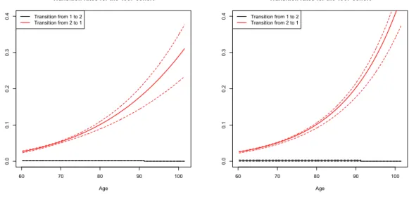
a log-likelihood of -14062.51 is obtained. The parameters are displayed in Table 3. We estimate the variance-covariance matrix of the parameters as before, both for Models 3 and 4. On this basis, we represent the estimated intensities and their associated pointwise 95%-confidence intervals in Figures 6 and 7 for transition be-tween groups and characteristic-specific death rates respectively. Let us first focus on the transition intensities between groups, see Figure 6. As expected when count-ing the number of observed transitions, the transition intensity α12(t) = b12 from

non-married to married is very low compared to the reverse transition 2 → 1, al-though it is not zero (see Table 3). We are here close to an irreversible multi-state model, but it is shown in Section 5 that the analogy is not completely valid since a small impact remains on stylized life insurance products.

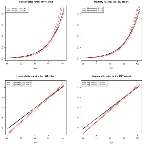
On the mortality compensation law Let us now focus on characteristic-specific log-mortality rates, see Figure 7. These show that for ages between around 60 and 85, mortality rates are lower for married individuals, which is intuitive. But after some age around 90, the situation is reversed, as for higher ages the mortality of married individuals becomes higher. This may be a suprising result at first sight, but in fact, this illustrates a well known demographic phenomenon referred to as the mortality compensation law. This appears when one compares several sub-populations at the same time, e.g. specific groups in a country or several national population, or the same population in successive time periods. It states that if the mortality factor is lower, namely here c23 < c13, then necessarily the age coefficient is higher, that

is d23 > d13 (see Table 3). In other words, a decrease of mortality at the lowest

ages in the age range leads to an increase of mortality at highest ages. Dynamically, for stochastic mortality models with a formulation closely related to Gompertz, such as Cairns et al. (2006), the times series of slope and intercept of log-mortality rates appear to be negatively correlated, as already highlighted in Strehler and Mildvan (1960). This phenomenon can be explained by the fact that the human life span, that is the maximum biological life length driven by the intrinsic rate of bodily deterioration, does not change much for reasonable time periods (see e.g. Strulik and Vollmer (2013)). Note that the compensation law can be also measured in two other ways, with their corresponding denominations: the compression of the distribution of ages at death, and the rectangularization of the survival curve. For further investigation of the compensation law and related effects, the reader is

(20)

referred to e.g. Strehler and Mildvan (1960), Fries (1980), Gavrilov and Gavrilova (1991), Wilmoth and Horiuchi (1999) and Strulik and Vollmer (2013). Note that as we avoid proportional hazard assumptions, we are able to reproduce such effects. This leads to several insights on the shape of aggregate mortality, as well as on the impact of life insurance products. This is developed in the next section.

Parameter Model 3 Model 4

p 0.329 0.329 a21 5.99 0.000397 b12 0.00194 0.00193 b21 0.0131 0.0693 c13 1.22e-05 1.23e-05 c23 2.96e-06 3.11e-06 d13 0.103 0.103 d23 0.119 0.118

Table 3: Estimated parameters for Models 3 and 4.

Figure 6: Estimated transition rates between groups for Model 3 (left) and Model 4 (right) with their 95 % confidence intervals

60 70 80 90 100 0.0 0.1 0.2 0.3 0.4

Age Transition from 1 to 2 Transition from 2 to 1 60 70 80 90 100 0.0 0.1 0.2 0.3 0.4

Age Transition from 1 to 2 Transition from 2 to 1

5 Aggregate mortality and the impact of

hetero-geneity on life insurance products

The aim of this section is to address the impact of the population dynamic hetero-geneity on (i) the aggregate mortality rate and (ii) typical life insurance products

(21)

5.1 Population heterogeneity dynamics

Figure 7: Estimated characteristic-specific death rates (top) and their logarithm (bottom) both for Model 3 (left) and Model 4 (right)

60 70 80 90 100 0.0 0.1 0.2 0.3 0.4

60 70 80 90 100 -5 -4 -3 -2 -1

Log-mortality rates for the 1907 cohort

Age Log-mortality rate from 1 Log-mortality rate from 2

60 70 80 90 100 -5 -4 -3 -2 -1

Log-mortality rates for the 1907 cohort

Age Log-mortality rate from 1 Log-mortality rate from 2

embedding life or death benefits. We begin by describing the dynamics of an het-erogenous population with specific composition.

5.1 Population heterogeneity dynamics

To understand the impact of the dynamic composition on several quantities of in-terest, one has to detail how a particular sample evolves through time, taking into account deaths but also characteristics changes during life. We see transition in-tensities αkl(t) depending on age t to be stochastic quantities as they depend on

the realized parameter vector θ, see (11), whose distribution can be approximated as detailed at the end of Section 3. We deal here with the mean trajectory of a given sample, therefore demographic stochasticity (which is a consequence of finite sample sizes) is not taken into account in itself. Let us recall that we are

(22)

inter-5.2 Aggregate mortality

ested here in the uncertainty in the parameters due to the finite sample data size and the interval-censoring mechanism. Let us denote g1(a) and g2(a) the initial

deterministic quantities (real numbers) of individuals in each group 1 or 2 with age a, which is nothing but the age of our sample of interest at the first census (here a = 37.25). Now, let us denote for t ≥ a, G(t) = g1(t)

g2(t)

!

the repartition between the two groups. Given the transition rates, this evolves (deterministically) according to deaths and characteristic changes. The classical Chapman-Kolmogorov equation gives us the average dynamics of our Markov process as

G0(t) = K(t)G(t), (12)

where the transition matrix K(t) is given by

K(t) = −α13(t) − α12(t) α21(t) α12(t) −α23(t) − α21(t)

! .

Note that the complexity of taking into account reversible transitions arises due to the fact that in general no analytical solutions are available for G (see e.g. Andersen et al. (1993)). This is also the case for the particular parametric forms we have chosen for the intensities. Indeed, since the matrices K(s) and K(t) do not commute3 we are not able to write an explicit formula for G(t). In practice, the assumption that the reverse intensity is zero is often used when a few number of such transitions occurred (see e.g. Czado and Rudolph (2002)). Although analytical solutions are not available in our case, we are able to compute the ordinary differential equation (12) numerically using a standard discretization scheme.

5.2 Aggregate mortality

In this part, our aim is to illustrate several patterns of aggregate mortality and explain them based on the analysis of the underlying population structure. Let us define the total number of individuals in the sample as

g(t) = g1(t) + g2(t). (13)

Note again that this is in fact a quantity in R+. Formally, the equivalent death rate

(in continuous time) is defined as µ(t) = −g

0_(t)

g(t) =

g1(t)α13(t) + g2(t)α23(t)

g(t) , (14)

which is nothing but an average of characteristic-specific death rates, whose weights depend on the dynamics of the underlying population composition.

(23)

5.2 Aggregate mortality

When looking at heterogeneity, a well known phenomenon is the fact that mor-tality rejoins the lowest one, more precisely: the aggregate death rate, that is the "equivalent" mortality force, gets closer to that of the group whose mortality is the lowest. This fact is naturally observed when individuals do not change between the groups. When characteristics changes are taken into account, the way aggregate mortality evolves through age may be different, and in particular even the reverse effect can be observed. The two applications we further develop below are able to capture such facts.

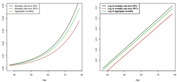
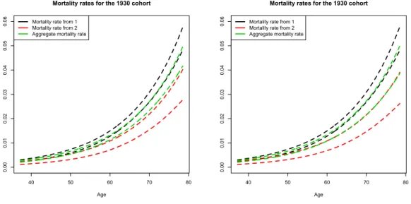
Socio-economic groups Aggregate mortality of Equation (14) is computed us-ing the dynamics (12), and the results are depicted in Figure 8 for the age range concerned with the estimation procedure. In this case, based on the initial sample proportions, and given the level of estimated transition intensities, aggregate mor-tality slowly rejoins mormor-tality of group 2, and the speed at which this effect occurs is quantified. This is crucial because it shows how a quantification of mortality at a deeper level leads to several insights on the shape of aggregate mortality. In our study, we were in addition able to capture the variance-covariance matrix of the parameters. Also, we can compute the associated 95%-confidence intervals, shown in Figure 9.

To further validate the modeling framework and the parametric assumptions, we can compare one hand the aggregate survival function obtained by taking into account the interval censoring scheme and the underlying heterogenous dynamics, and on the other hand the survival function computed on the sample regardless of individual characteristics, e.g. by Kaplan-Meier estimator. This comparison is shown in Figure 10 for Models 1 and 2. Note that the two curves shapes and levels are very similar, although they may differ at high ages for extreme scenarios. This could be explained by the Gompertz assumptions for mortality which is not a good approximation for ages around 40 years, which may result in a slight underestimation of mortality. Nevertheless, we believe that this is the best parametric option for the whole age range and given the small amount of data. Note also that despite these differences in some parameter scenarios, we capture on the other side more information on the heterogenous dynamics, which is at the core of our study. Marital status The study of the underlying population composition gives us many insights on the age pattern of aggregate mortality. This is particularly the case for the focus on marital status. In Figure 11, we depict the characteristic-specific and aggregate log-mortality rates for Models 3 and 4, as well as their corresponding 95%-confidence intervals in Figure 12. Let us describe the age pattern of aggregate log-mortality: at age around 60, this quantity is closer to the "married" mortality, then rejoins the "non-married" mortality at age around 85 and remains at this level until

(24)

5.2 Aggregate mortality

the end of the age range considered. This fact can not be described as "aggregate mortality rejoins the lowest one", due to the impact of the evolving population composition taking characteristics changes into account. Here, aggregate mortality first rejoins the highest one, and then stays at the level of the "non-married" group since it corresponds to the characteristic which is more and more represented in the population due to characteristic changes at high ages.

For this study on marital status also, to further validate the modeling framework and the parametric assumptions, we plot in Figure 13 the comparison between the aggregate survival function obtained by taking into account the interval censoring scheme and the underlying heterogeneity, and also the survival function computed on the sample regardless of individual characteristics, e.g. by Kaplan-Meier estimator. In this case, survival curves are really similar, showing that our method captures the underlying heterogeneity that furthermore replicates the overall mortality observed in the sample.

Figure 8: Characteristic-specific and aggregate mortality rate (left) and their loga-rithm (right) for Model 1.

40 50 60 70 80 0.00 0.01 0.02 0.03 0.04 0.05

Age Mortality rate from SPC-Mortality rate from SPC+ Aggregate mortality 40 50 60 70 80 -5 .5 -5 .0 -4 .5 -4 .0 -3 .5 -3 .0

Age Log of mortality rate from SPC-Log of mortality rate from SPC+ Log of aggregate mortality Log of mortality rate from SPC-Log of mortality rate from SPC+ Log of aggregate mortality

(25)

5.3 Impact on life insurance products

Figure 9: Characteristic-specific and aggregate mortality forces 95%-confidence in-tervals for Model 1 (left) and Model 2 (right).

40 50 60 70 80 0.00 0.01 0.02 0.03 0.04 0.05 0.06

Age Mortality rate from 1 Mortality rate from 2 Aggregate mortality rate

40 50 60 70 80 0.00 0.01 0.02 0.03 0.04 0.05 0.06

Age Mortality rate from 1 Mortality rate from 2 Aggregate mortality rate

5.3 Impact on life insurance products

The aim of this section is to assess the impact of heterogeneity on life insurance products as death or life benefits. Particular attention is devoted to characteristics changes and parameter uncertainty. Let us start with a portfolio with some compo-sition G(a) = g1(a)

g2(a)

!

, and focus on two simplified actuarial quantities as the life benefit and the death benefit, that start at age a and end at age ¯a. Let us consider a constant interest rate r. The life benefit, also known as annuity contract, amounts to pay 1 per time unit to still alive individuals until age ¯a, that is

LB := Z ¯a

a

e−r(t−a)g(t)dt,

where g(t) is defined in (13). Another quantity of interest is the death benefit, which pays 1 at each death before age ¯a. Note that formally, the number of deaths in the time interval [t, t + dt) is g(t) − g(t + dt) ≈ −g0(t)dt. Then the death benefit, also known as term insurance contract, is rigorously defined as

DB := − Z a¯

a

e−r(t−a)g0(t)dt.

After integration by parts, it can also be rewritten in terms of the life benefit as DB = g(a) − e−r(¯a−a)g(¯a) − rLB.

This gives another interpretation of the death benefit: it amounts for the insurer to pay 1 at each individual in the portfolio (first term), then take back 1 from each

(26)

Figure 10: Survival curves 95%-confidence intervals obtained in Model 1 (left) and Model 2 (right) compared to the Kaplan-Meier estimate

0 10 20 30 40 0.5 0.6 0.7 0.8 0.9 1.0 Kaplan-Meier estimator Aggregate mortality 0 10 20 30 40 0.5 0.6 0.7 0.8 0.9 1.0 Kaplan-Meier estimator Aggregate mortality

individual which is alive at the end at age ¯a (second term), and finally that each alive individual pays back r per time unit to the insurer (third term).

The aim now is to compute the distribution of the life and death benefits, which depends on the (random) set of parameters, under several configurations. In partic-ular, we measure sensitivities due to (i) the composition of the initial population, (ii) the fact that characteristics changes are taken into account or not, and (iii) several values for the interest rate r.

Impact of socio-economic heterogeneity Let us fix a = 37.25 and ¯a = 78.5, corresponding to the age range considered in the estimation procedure. This is typical of death benefits, therefore numerical results are given in this context. The set of parameters is given as follows:

(i) the initial population at age a= 37.25 is made of SPC+ (group 2) only (p = 0), or representative of the initial sample (p = 0.703), or made of SPC- (group 1) only (p = 1).

(ii) the random distribution of the value of the death benefit is represented using the full model (12) and compared to the same where characteristics changes are not taken into account (that is α12(t) = α21(t) = 0).

(iii) two values for the interest rate are tested, namely r = 1% in Figure 14 and r = 3% in Figure 15.

These results are depicted for both Models 1 and 2.

Let us first focus on the initial population that is representative of the origi-nal sample composition (p = 0.703), see the middle column in Figures 14 and 15. From this test, it appears that considering characteristics to be stable slightly

(27)

over-5.3 Impact on life insurance products

Figure 11: Characteristic-specific and aggregate log-mortality rate for Model 3 (left) and Model 4 (right).

60 70 80 90 100 -5 -4 -3 -2 -1

Log-mortality rates for the cohort born in 1907

Age Log-mortality rate for non-married Log-mortality rate for married Log of aggregate mortality

60 70 80 90 100 -5 -4 -3 -2 -1

Log-mortality rates for the cohort born in 1907

Age Log-mortality rate for non-married Log-mortality rate for married Log of aggregate mortality

estimates the value of the death benefit, in other words under-estimates the sample size, or equivalently over-estimates mortality. Therefore, it seems that the propor-tion of individuals in group 1 is over-estimated when characteristics changes are omitted. Yet, let us recall that the transition intensity from 1 to 2 is on the whole lower than 2 to 1, see Figure 4. But in fact, the total intensity of characteristics changes from group 1 to group 2 is the product of the 1 → 2 transition intensity times the number of individuals in group 1. Therefore, when the initial proportion of group 1 is sufficiently large, the number of changes from 1 to 2 becomes higher than those from 2 to 1, and the death benefit is over-estimated if changes are not taken into account. This can be illustrated if we start from a population initially made of group 1 individuals only (p = 1), see the right column in Figures 14 and 15. On the contrary, if the proportion of group 1 individuals is lower enough, the death benefit is under-estimated when considering characteristics stable during life. This is illustrated when starting with group 2 individuals only (p = 0), see the left column in Figures 14 and 15. Note that of course, the death benefit is naturally lower with individuals in group 2 compared to group 1, and our modeling framework quantifies the difference between the two.

As for the comparison between the two Models 1 and 2, results are very similar, both in terms of overall level and uncertainty. Finally, comparing Figures 14 and 15 allows us to test the sensitivity to the interest rate in each scenario. As expected, the value of the death benefit (x-axis) decreases as r increases, but in each scenario taking into account transitions between groups still has a huge impact.

(28)

Figure 12: Characteristic-specific and aggregate log-mortality forces 95%-confidence intervals for Model 3 (left) and Model 4 (right).

60 70 80 90 100 -5 -4 -3 -2 -1

Log-ortality rates for the 1907 cohort

Age Log-mortality rate from 1 Log-mortality rate from 2 Aggregate log-mortality rate

60 70 80 90 100 -5 -4 -3 -2 -1

Log-ortality rates for the 1907 cohort

Age Log-mortality rate from 1 Log-mortality rate from 2 Aggregate log-mortality rate

Impact of marital status heterogeneity Concerning marital status hetero-geneity, numerical results also show that it is crucial to take into account both characteristic-specific mortality and transitions between states. Let us fix a = 60.25 and ¯a = 101.5, corresponding to the age range considered in the estimation proce-dure, typical of a life benefit. For these results, the set of parameters is given as follows:

(i) the initial population at age a = 60.25 is made of married individuals (group 2) only (p = 0), or representative of the initial sample (p = 0.329), or made of non-married individuals (group 1) only (p = 1).

(ii) the random distribution of the value of the death benefit is represented using the full model (12) and compared to the same where characteristics changes are not taken into account (that is α12(t) = α21(t) = 0).

(iii) two values for the interest rate are tested, namely r = 1% in Figure 16 and r = 3% in Figure 17.

These results on life benefits are depicted for both Models 3 and 4. The impact of transitions out of marriage is clear, being mostly at these ages transitions from married to widowed. This is depicted in Figures 16 and 17 when starting with mar-ried individuals (left column) or a population which is representative of the original sample (middle column). On the contrary, as the transition intensity from non-married to non-married is small, the impact is not so important when starting from non-married individuals only (right column). But let us emphasize that a difference still remains, which can have a real impact when multiplied by a huge amount of pensions. Also here, when comparing Models 3 and 4, the main difference appears to be the uncertainty about the life benefit value, this one being lower in Model 4; in

(29)

Figure 13: Survival curves 95%-confidence intervals obtained in Model 3 (left) and Model 4 (right) compared to the Kaplan-Meier estimate

0 10 20 30 40 0.0 0.2 0.4 0.6 0.8 1.0 Kaplan-Meier estimator Aggregate mortality 0 10 20 30 40 0.0 0.2 0.4 0.6 0.8 1.0 Kaplan-Meier estimator Aggregate mortality

this model, also less performing than Model 3 in terms of likelihood (see Subsection 4.2), confidence intervals are in fact lower both for mortality rates (see Figure 7) and transitions rates between states (see Figure 6).

To conclude these numerical results assessing the impact of socio-economic or marital status heterogeneity on typical life insurance products, let us emphasize that the impact of taking into account characteristics changes depends on both the initial population composition and the level of the several possible transition intensities. The maximum likelihood procedure developed in this paper that takes into account interval censoring allows us to quantify such effect based on longitudinal data.

Conclusion

In this paper, we have developed a parametric maximum likelihood method for mea-suring mortality heterogeneity when characteristics changes are interval-censored, which is a particularity of longitudinal data based on censuses. Indeed, for such data individuals are often observed at isolated points in time so the times at which characteristics change during life remain unknown. While applying such a method to a representative sample of the French national population, which presents both a small number of individuals and a systematic interval-censored observation mech-anism, we were still able to capture characteristic-specific mortality rates linked to socio-economic groups or marital status, as well as to measure the transition rates between the groups. Special attention was devoted to parameter uncertainty whose magnitude differed depending on the characteristics and the transition rates

(30)

Figure 14: Death benefit distribution with r = 1% and p = 0 (left), p = 0.703 (middle) and p = 1 (right) for Model 1 (top) and Model 2 (bottom)

0.20 0.25 0.30 0.35 0.40 0 10 20 30 40 50

Distribution of death benefit Multistate model

Without transition between groups

0.20 0.25 0.30 0.35 0.40 0 10 20 30 40 50

considered.

Based on such estimates, we highlighted effects such that the mortality com-pensation law between groups. We also addressed the dynamic evolution of several populations with specific compositions, leading us to get insights on the age pat-tern of aggregate mortality related to the underlying dynamic heterogeneity. We were also able to quantify the impact on typical life insurance products of consider-ing characteristics stable durconsider-ing life instead of takconsider-ing into account their variability. Interestingly, this impact depends on both the initial population composition and the level of the transition intensities between groups; these insights are crucial for longevity/mortality risk management.

The statistical estimation of mortality heterogeneity based on complex data re-mains a challenging field of actuarial research. Further improvements would concern higher dimensional multi-state models with more groups, as well as the estimation of several cohorts simultaneously. To this aim, "larger" datasets are required, first including more individuals to allow to increase the number of possible states, and sec-ond with more frequent and deep records leading to reasonable observation schemes and time windows, since particularly the study of the age pattern of heterogenous mortality within real cohorts requires very long historical data.

(31)

Figure 15: Death benefit distribution with r = 3% and p = 0 (left), p = 0.703 (middle) and p = 1 (right) for Model 1 (top) and Model 2 (bottom)

0.15 0.20 0.25 0 20 40 60 80

0.10 0.15 0.20 0.25 0.30 0 20 40 60 80

Aknowledgements

The authors are grateful to Philippe Saint-Pierre for several enlightening discussions on this work. The authors also thank Jacques Portes for his help on using computer resources at LPMA, as well as Catherine Mathias, Olivier Lopez, Xavier Milhaud, Quentin Guibert and Julien Tomas for fruitful discussions on several topics related to this work.

(32)

REFERENCES

Figure 16: Life benefit distribution with r = 1% and p = 0 (left), p = 0.329 (middle) and p = 1 (right) for Model 3 (top) and Model 4 (bottom)

20.0 20.5 21.0 21.5 22.0 22.5 23.0 0.0 0.5 1.0 1.5 2.0 2.5 3.0 3.5

Distribution of life benefit Multistate model Without transition between groups

20.0 20.5 21.0 21.5 22.0 22.5 23.0 0.0 0.5 1.0 1.5 2.0 2.5 3.0 3.5

20.0 20.5 21.0 21.5 22.0 22.5 23.0 0 1 2 3 4 5

References

Aalen, Odd O, Søren Johansen. 1978. An empirical transition matrix for non-homogeneous markov chains based on censored observations. Scandinavian Journal of Statistics 141–150. 2

Andersen, Per Kragh, Ørnulf Borgan, Richard D Gill, Niels Keiding. 1993. Statistical Models Based on Counting Processes. Springer-Verlag, New York. 2, 21

Bensusan, Harry, Alexandre Boumezoued, Nicole El Karoui, Stéphane Loisel. 2010-2015. Bridging the gap from microsimulation practice to population models: a survey. Work-ing paper . 2

Boumezoued, Alexandre. 2015. Macroscopic behavior of heterogenous populations with fast random life histories. Working Paper . 2

Cairns, Andrew JG, David Blake, Kevin Dowd. 2006. A Two-Factor Model for Stochastic Mortality with Parameter Uncertainty: Theory and Calibration. Journal of Risk and Insurance 73(4) 687–718. 18

Commenges, Daniel, Anne Gégout-Petit. 2007. Likelihood for generally coarsened observa-tions from multistate or counting process models. Scandinavian journal of statistics 34(2) 432–450. 4

Commenges, Daniel, Pierre Joly, Anne Gégout-Petit, Benoit Liquet. 2007. Choice between semi-parametric estimators of markov and non-markov multi-state models from coars-ened observations. Scandinavian Journal of Statistics 34(1) 33–52. 4, 5, 13