HAL Id: hal-01365737
https://hal.archives-ouvertes.fr/hal-01365737
Submitted on 13 Sep 2016
HAL is a multi-disciplinary open access
archive for the deposit and dissemination of
sci-entific research documents, whether they are
pub-lished or not. The documents may come from
teaching and research institutions in France or
abroad, or from public or private research centers.
L’archive ouverte pluridisciplinaire HAL, est
destinée au dépôt et à la diffusion de documents
scientifiques de niveau recherche, publiés ou non,
émanant des établissements d’enseignement et de
recherche français ou étrangers, des laboratoires
publics ou privés.
Module GYPTIS version 1.0 : contact unilatéral avec
frottement en mécanique des structures, inéquations
variationnelles
Jean-Claude Latil, Michel Raous
To cite this version:
Jean-Claude Latil, Michel Raous. Module GYPTIS version 1.0 : contact unilatéral avec frottement en
mécanique des structures, inéquations variationnelles. [Rapport de recherche] Publications du LMA,
numéro 132, LMA. 1991, 93 p. �hal-01365737�
Légende
de la figure
de couverture :
Le problème
du contact
de deux solides.
ISSN 0750 - T356
PUBLICATIONS
DU L.M.A.
n° 132 (juin 1991)
NOTES
SCIENTIFIQUES
MODULE GYPTIS VERSION 1.0
CONTACT UNILATERAL AVEC FROTTEMENT
EN MECANIQUE DES STRUCTURES
INEQUATIONS
VARIATIONNELLES
Jean-Claude
LATIL et Michel
RAOUS
1
MODULE GYPTIS VERSION 1.0
CONTACT UNILATERAL AVEC FROTTEMENT
EN MECANIQUE DES STRUCTURES
INEOUATIONS VARIATIONNELLES
Jean-Claude LATIL et Michel RAOUS
Centre National de la Recherche Scientifique
Laboratoire de Mécanique et Acoustique
3
I - INTRODUCTION
Le module GYPTIS permet de résoudre des problèmes de con-
tact unilatéral avec frottement de Coulomb entre une structure
et un obstacle fixe ou entre différents solides déformables. Le
problème est ici posé et résolu pour de petites déformations
élastiques. L'extension à la viscoélasticité, la viscoplastici-
té ou l'élastoplasticité en grandes déformations a été réalisée
par ailleurs (voir références [2], [3], [4] ci-dessous).
Il s'agit de problèmes pour lesquels l'état de contact
est inconnu, c'est à dire qu'à la fois l'étendue exacte de la
zone de contact et les forces de contact font partie des varia-
bles du problème. Le contact unilatéral, c'est à dire la condi-
tion de non pénétration, s'écrit sous la forme d'un problème de
complémentarité ( problème de Signorini ). La loi de frottement
est celle, classique, de Coulomb, loi à seuil lié à la force
normale de contact dépendant de la solution : ceci explique le
caractère implicite du problème posé. Cette loi de Coulomb est
utilisée ici sous sa forme non régularisée et ceci est un point
important de la méthode numérique proposée qui la différencie
des méthodes de type compliance ou pénalisation.
Le formalisme adopté est celui des inéquations variation-
nelles. On trouvera dans la référence [1] les détails concer-
nant le modèle, son expression mathématique et sa résolution.
Cet article fait l'objet du paragraphe II.
Le problème se pose sous sa forme la plus naturelle en
termes d'inéquation variationnelle implicite ( ou sous forme
d'inéquation quasi-variationnelle si on l'écrit sous sa forme
duale ). Moyennant l'introduction d'un problème de point fixe
sur le seuil de glissement on se ramène à la résolution du pro-
blème couplé associant le point fixe sur le seuil de glissement
à la résolution d'un problème d'inéquation variationnelle cor-
respondant en fait à un problème de Tresca. On notera la pré-
sence d'un terme non différentiable ( la valeur absolue des dé-
placements tangentiels de contact ) provenant du frottement.
Grâce à la symétrie de l'opérateur d'élasticité, le pro-
blème est ici posé et résolu sous la forme d'un problème de mi-
nimisation sous contraintes ( sur un convexe défini par la con-
dition de non pénétration ). On se limite à l'utilisation
d'éléments PI droits qui conduisent à un problème approché bien
non pénétration sous forme produit : la projection
alors simplement composante par composante.
On utilise une technique de projection associée à la mé-
thode de surrelaxation. L'aspect relaxation ponctuelle ainsi
que la séparabilité du convexe discrétisé en espace produit
font de la méthode SORP ( Successive Over-Relaxation with Pro-
jection ) un procédé facile à mettre en oeuvre et assez robus-
te. La vitesse de convergence dépend du choix du coefficient de
relaxation. Il n'y a pas d'estimation théorique d'une valeur
optimum de ce coefficient dans le cas avec contraintes traité
ici. Si plusieurs calculs sont effectués sur un même maillage,
une recherche dichotomique de cette valeur optimum est recom-
mandée. Sinon, on suggère une valeur comprise entre 1.50 et
1.95. On notera toutefois que la convergence est moins sensible
à la valeur de ce coefficient dans le cas avec frottement que
dans celui sans frottement : ceci provient du fait que les ité-
rations de point fixe sur le seuil de glissement impliquent de
toute manière un nombre d'itérations de relaxation plus élevé.
En ce qui concerne ces itérations sur le seuil de glissement g,
le procédé diagonal utilisé est le suivant : pour les premières
itérations sur g, une résolution grossière est effectuée, et la
résolution fine sera menée à terme seulement à l'approche de la
détermination précise de g. Un gain de trois à quatre est ainsi
obtenu sur le temps total de résolution.
Un procédé de condensation est aussi proposé dans GYPTIS.
Il s'agit, par une inversion partielle de la partie linéaire du
système, de poser le problème non linéaire sur les seules va-
riables de contact et de travailler ainsi sur une matrice plei-
ne mais de taille réduite.
Nous utilisons également :
- un procédé d'accélération de Aitken qui ne nécessite pas de
choix particulier du coefficient optimum,
- une méthode de programmation mathématique de Lemke-Cottle-
Dantzig qui est une méthode directe très performante.
Ces méthodes, de développement récent, feront l'objet
d'extensions ultérieures du module GYPTIS.
Il en sera de même pour les méthodes multigrilles mises
en oeuvre sur ce type de problèmes dans l'équipe Mécanique et
Méthodes Numériques au Laboratoire de Mécanique et d'Acousti-
que [5].
Le module proposé ici a été largement testé sur un cer-
tain nombre de Benchmarks, définis notamment par le Groupe va-
lidation de codes de calcul du GRECO Grandes Déformations et
Endommagement. Il a été également utilisé sur un certain nombre
d'applications de type industriel ( assemblage de structures,
5
[1] RAOUS M., CHABRAND P., LEBON F., 'Numerical methods for
frictional contact problems and applications', J. Mec.
Theor. Appl., n° spécial, supplément au vol. 7, 111-128,
1988
[2] RAOUS M., 'Contacts unilatéraux avec frottement en visco-
élasticité', in "Unilateral Problems in Structural Analy-
sis", Ed. Pr. Maceri, Del Piero, C.I.S.M., Springer-Verlag 1985
[3] RAOUS M., LATIL J.-C., 'Code d'éléments finis pour des
problèmes contact unilatéraux avec frottement formulés en
termes d'inéquations variationnelles', in "Unilateral Pro-
blems in Structural Analysis", Ed. G. Del Piero, C.I.S.M.,
n° 304, Springer-Verlag, 1987
[4] CHABRAND P., PINTO Y., RAOUS M., 'Numerical modelling of
the friction in small and finite strains for metal forming
processes. Analysis of the blackholder function', Euromech
273 : Unilatéral Contact and Dry Friction, La Grande Motte
29 Mai-ler Juin 1990
[5] LEBON F., RAOUS M., LATIL J.-C., GREGO L., 'Multigrid me-
thods in non linear structure mechanics', Conférence Euro-
péenne sur les Nouvelles Avancées en Calcul des Structures
7
Journal de Mécanique théorique et appiiquér, Journal of theoraied and appiied mechmucs Special issue, suppiement n° 1 to vol. 7 - 1988
Numerical
methods
for frictional
contact
problems
and applications
M. RAOUS, P. CHABRAND et F. LEBON
Centre National de la Recherche Scientifique Laboratoire de Mécanique et d'Acoustique
13402 Marseille Cedex 9, France et
GRECO Grandes Déformations et Endommagement
Résumé - Nous présentons ici une synthèse des différentes méthodes numériques développiez au laboratoire ces dernières années pour résoudre les problèmes de contact unilatéral avec frottement. Les formulations variationnelles classiques associées au cas statique sont étendues au cas de chargements quasi-statiques complexes par l'introduction de termes en vitesse dans ces formulations. La généralisation aux problèmes de viscoélasticité et viscoplasticité est donnée. Les méthodes utilisées pour le contact sont de différents types : relaxation avec projection, programmation linéaire, point fixe sur conditions aux limites par pénalisation. Des techniques d'amélioration des performances des algorithmes sont présentées. L'efficacité des algorithmes est discutée sur des exemples test, et des applications à des exemples de type industriel sont présentées.
Abstract - Ae présent a synthesis of the dirferenc nta»rical mathods devalopped chesa lasr few years in the laboracory to solve frictional unilatéral contact problems. The classical variational formulations assoclared co the stitic case are extended co complex quasi-stacte loiding cases by che use of velocity torms in the formulations. A generalization for viscoelasticicy and viscoplasticity is given. Concacc is désir wich by che use of différent numerical mathods : relaxation vich projection, machematical programsing, fixed point on boundary conditions through penalizacion. Techniques for
improving the algorithms are presented. Their efflciency is dlscussed on test examples and applieations conceming induscrial problems are presented.
1. INTRODUCTION
Contact problans are caracterized by non linear relations between displacements, or rates of déplacement and forces on a part of the boundary. The real contact area and the contact forces are unknown a priori and have to be decer�tined by solving the whole problem. They are caracterised by a set of inaqualities vhich lead to a complémentarité problem (1). In elasticity, the assoeiat:ad variational forma is set as an implicit variational inéquation. An extension is given for viscoelasticity and viseoplasticity by introducing a coupling vith a linear or non linear différenciai équation.
The model is generalized to several body contact problèmes. Duvaut [2J gava a formulation of the Signorini problem vit friction for the static case. Ve first give numerical méthode based on punctual relaxation to solve this problem. Différent 10URNAL DE MÉCANIQUE n9oaJQUE ET APPLIQUEEJJOUIWAL OF THEORET1CAL AND Apnmm MECHANtC3
M. RAOUS et al.
aecelerating processes are used to as to obtain a poverfull algorithm even for large dimensional probles. A generalization for quasistatic évolutive problems is given. A velocity formulation leads to an incrément*! form solved by a stop by step algorichm using the previous numarical techniques. For frictionlesa problems, mathematical programming 9ethods are also used (1). The efficiency is appreciated on a few test examples provided by a group of the GRECO 'Grandes Déformations et Endommagement' and applications to industrial exemples are presonted.
2. THE SICNORINI PROBLEK VITS FRICTION
go first set a unilaterai contact probleu becween an elastic solid and a rigid obstacle for the static case under swll transformation hypothesis. It is a Signorini's probleu with friction (2). 41e denote by 17 the open set liaiting the solid. Its boundary CM is separated as follows XI - rI U I~2 U r On rI, va impose homogeneous boundary conditions. On I"2 , a force dansity 92 ta applied. The part rz is concerned by the contact with the rigid obstacle. Iia denote u the displacement field. On rz' we partition the vector u (in fact in the sense of the trace of u) and the density contact force vector F into normal and tangential compononts (n ta the exterior normal unit vector to 1-,)
u - un + uT, F-F�n+ + F, (1) In n, a force density �01 , and a thermal strain are prescribed oo X(6-6o) ; X is the dilatation censor, 8 the actual temperature field and 9, the initial one.
Uniliteral conditions
The unilateral condition::, vritten on thé part 1�� of the boundary, lead to the following complementarity conditions
us � 0, F, � 0, ... F. - 0 (2) The case lu � - 0, F." 4 0) charaeterizes the contact zone and the lu" � 0, Fu - 0) corresponds to the separate part.
Note 1 : for this formulation. r, is defined as the initial real contact area and only a loss of contact on rz will be allowed. The extension of the contact area cannot be modelized by those relations, -tore generally, we could write :
us, - a � 0, F, � 0, (u. - a) F, - 0 (3) where a ta a given funetion defined on
i'� as tM initial distance of each point of r, to the obstacle. For large displacements a satisfactory définition of et ta a serious probleu, but under a small transformation hypotheais there ta no ubiguity and the distance may be defined according either to the normal to the solid or the normal to the obstacle. lie have to note that undar a small transforfation hypothenis, relations (3) are incorrect bocause u, ta an infinitesimal funecion and a a finite one. Neverthelesa, this will be used in the numerical modal.
Friction conditions
Ue use hère the clantical Coulomb friction lav. In apite of its ale»ntary fora, this friction law is capable of describing correctly numerous problème involving dry friction (especially for metal/metal contact) as long as the numerical treatement is carefully effected (see expérimental comparison (29J). It is clear that lubrificated contact or probleus involving very high temperatures will need more sophisticated lava The Coulomb friction law is formulated :
9
NUMERICAL METHODS FOR FR1CTIONAL CONTACT
4 IFUI I (4)
IFr 1 � W IFs I » ut - 0 (5) IFr 1 - .. IF.I .. � - -Á Fr k � 0 (6) The dot dénote* the tine relative derivation, and 1s ia the friction coefficient.
Note 2 : the no-contact situation (F.-F. -0) is vell described because the colinearity condition (6) betwoon �.r and FT (which is zero in this case) is tbm sacisfied for any Úy. Note 3 : in the case of the unilateral conditions under consideration, the inequalities (3) enable us to replace IF, by -F, in the relations (4)(5)(6).
Folloving Duvaut (21, this friction law can be vritten for static cases
IFT 1 4 4 IF, 1 (7)
IFt I � W IF� 1 » uT - 0 (1) IFT 1 - w IFe I » uT - -a' FT A' � 0 (9) Frou a mechanical point of view, the validity of this static modal is very limited because friction is clearly a path dependant phénomena which has to be set on displacement velocities. Nevercheless, the numerical methods for solving this problem will be used in the resolution of che inéremental problem derived froa the general relations (4)(5)(6). So we firsc focus on the fillowing static formulation :
Problem Pl :
Be given the loads (q)1' 9, ) E (Lz (O»3X (Lz (rz»3 ,the prescribed strain eOE(Lz (0»' Find che déplacement u E (H �(O»3-
/v E (Hl(0»3; v - 0 on rz},the strain e E al�fl))6, che stress a E (L2 (fl))* , the contact force density F
E (H-�(rz»3 such that :
�u 2" l (UI.J+ uJ.I) + �U
(10)
a. J. J - -q)11 in n
(11)
o n - -�p2l onr2 (12) oi ,� i n� - � F , 1 on ! � 2 (13) uy - KIJkl"'¡ in 0 (14) and verifying the unilateral conditions (2) and the friction relations (7)(8)(9). Kijk te the elanticity coefficients.In other papers (Raous [41[5), Bouc and al. [6]). détails can be found on the differenc cholces of the funetional scheme, the functional sets and the duality produits which allou to set the problem under the folloving variational fora :
Problème P2 : Let
(q)1 ,q)zl and ec be given as in problem Pl
Find u E K - v v E (Hô ((1) ) � ; v, � 0 on r3} such thac :
V v E K a(u,v-u) - (f,v-u) + j(v,u) - j(u,u) � 0 (15) wlth : a(u,v) -
Jn (Dv]°K(Du)dx (16) (£'v)
:- Jn vd. + Irz �v d'Y + Jn IK«oll[Dv)dx (17) j(u.v) -
F 1i IFh (u) 1 1 VT 1 dr
(11)
M. RAOUS et al.
D is the symmetrical gradient mapping.
This problem is an implicit variational inequation because of the tere J(u,v) in which F, dépends on the solution . Though the convex cone K does not dépend here on the solution, the nature of the problem is the same as that of a quasi-variational inequation. In fact, the dual formulation of problem P2 is a quasi-varlational inéquation : the unknovn force density Fr is supposed to remain in the polar coi» K* depending on M- IF( I .
Through a fixed point method on the sliding limit IF ,(u)I, we get a more classical variational inequacion (see Panagiotopoulos [7]). Iie thug introduce a Tresca's friction problem. the sliding limit funccion g defined on r, boing the new variable.
Problem P3 : Find fixe point of the application g - �IF.(u)1
where u is solution of the problem P4 depending on g Problem P4 : Let
1�1�1 ,�I�z ), e° be given as in problem P1. Let g E Lz(1-z), find u E K such that :
V v E K a(u,v-u) - (f,v-u) + j(v) - j(u) � 0 (19) rhere (v) -
frz glvTl dY
(20)
go nov have to solve the variational inequation problem P4 including the undifferentiable tera (20). Thanks to the sysm try of the bilinear form a(.,.), va can write the problem P4 under the following équivalent minimization problem wich constraints: Iroblem PS : Let
1�1�1' pzl, e° and g be given as defined in problem P4, Find u E K such that :
V v E K e (u) � � (v) (21) rit :
(v) - 2 a(v,v) - (f,v) + j(v) (22) "Iote 4 : The Coulomb friction problem is solved through the intermediate resolution of a séquence of Tresca's problème. We vould like to undarline that a Tresca's model, alone, vould not be adéquate for a problem involving unilatéral conditions : g needs to be equal co zero on che non contact parts (u, strictly négative) and these parts are unknovn a priori. Tresca's friction is adequate only in very simple cases where the contact area and the normal contact forces are knovn a priori.
Mathomticel renards
The existence and uniquenens of the solution of the Signorini problem have been proved by Fichera (81, Stampacchia (9) thanks to an extension of the Lax-Milgran theorem. The static Tresca problem or the Coulomb problem with a given F. (see Duvaut j2j) also have a unique solution : they are not unilatéral problems, the contact area is given. The existence and uniquenass for the unilatéral problem including static Coulomb's friction (i.e. probleu P2) are not proved. The difficultés arine froa the fact that F, which is unknom in this problem. belongs to H~ *(!"") (this lands to compacity problems...). In che other proble» , this given force is choosen only in L1 (F) Nevertheless on the regularized problem introduced by Duvaut 121. Oden-Pires [11), Cocu (12), existence is proved and unicity is obtained for small friction coefficients. This concerns a non local friction law (Duvaut defines F. chrough a convolucion with a smooth function with compacc support).
11
NUMERICAL METHODS FOR FRICNONAL CONTACT
3. !lUL2IEODT CONTACT FIOILIX (SEXE [ 13 J ) Let A and B be two deformable solids occupying the open sets n" and ÇP . . Soundary conditions are set on 11 and 11 ' volumic force densities Pi and IP ', are applied in i7" and ÇP , , surfacic force dansities 40, and d are given on Fj and r* . The contact aroas are 1� and I1 . P and Q denote an opposite pair of points of r* and £1 as deseribsd on figure 1. 'lhe unit vector nA and nl are still the
external vectors to n, and I1 . figure 1 : tvo body contact probleu Unilatéral conditions
Under a saall transformation hypothasis, va write the unilatéral problem as:
-;, 4 Il 0. Fj- Fjj. FI.' 19 0. (u:, �).F: - 0 (23) We have shovn in (16) that this problem is still a complementarity problem thanks co a convenient choice of the duality product betveen the trace spaces.
Friction condition
The static Coulomb friction lav can be vritten :
F;- � (24)
1r;1 �... 1r:1 1 (25) 1 FTP 1 � �aIF� I �� uj+ uj - 0 0 (26) IF* 1 - la 1 FVP .3 3 à � 0 such that t 4 + 4 -a fr (27) This problem vlll be treated after discretization by a change of variable (see [13). Ut will see in paragraph 7 the application to a multibody contact problen.
4. VARIATIONAL FORMULATION FOIL QOASI·S?A?IC Pa0BLOlS
iTe first set the quasi-static problem using the général Coulomb friction lav (4)(5)(6) (written in uni of rates of displac...nt) in the ease of a given contact boundary (no unilatéral conditions). For an évolutive problon, it is clear that friction is an irreversible phenomena which has to be rritten in teras of rate* of displacement. It is a path dépendant phenomena and the final solution doas not dépend only on the final force star* but on all the intermediate states.
Problem P6 :
Se Siven the force...1'. z) : [O.Tl - (LZ(O»3X (L2(rz»3, the thermal strain e°: (0,T] � (L=(L1))°,find u : [0,T] � (Hô(I1))ssueh that :
for t - 0 u(O)-u. be given in 0
for t E ]O,Tl (10)(11)(12)(13)(14) and (4)(5)(6) be verified.
Restricting the dynanical formulation of Duvaut-Lions [2] to the quasi-static case, we remove the inertial taras and ve get the folloving variational formulation.
M. RAOUS et al.
Problem P7 :
1��, �21 and e° be given as in problem P6, find u(t) E U - (H�(n»3 such that : for t - 0 u(O) - Uo be given in n
for c � ]O.T) V v E U a(u,v-�)-f(v-û)+j(v)-j(û) 0 0 (28)
In view of the numerical resolution, ve give nov an incremental formulation by appro- ximating the derivativez by finite différences. Lot ( tQ , .. , t^ , .. , t^ I be a partition of che interval (O,T], va get a forvard finité difforence approximation of u by :
Substituting u(t,,) by u* and f(c1') by f and setcing
Ovi- uk'1 - uk and Ac* - t" 1 tr , va vrite (28) under the following font :
a(u=+ �k,�-�') - (fi + W V-4Uk) + j(v) - j(Gu`� z 0 (30) a(�k.�-�) - (Aft,v-tJ.) + j(v) - j(�t) � - �(UI, V_tU,, + (fr, v-Dy) (31) The left part of the inequality (31) is conmected to che equilibrium deflecc Rk, i.e. the friction force at the previous time ri.
-�(u',v-4�u') + (f;.�-4f) - (R'.v-Aj1) (32)
Sc, we get a problem formally analogous to the static case one :
Problem P8 :
find �� U such that
V v E U a (àuk , v - 6LLà (Rt+ Afk.� - �) + j(v) - j(dux) k 0 (33)
The non pénétration condition corresponding to the initial unilateral problem is introduced by projecting tuk such as to assume
uk + àuk 0 0 (34)
Consequently, we have to solve problem PB which is of the same form as the static problem P4. Ue note that we have for each step an extra load coming from the friction force of the previous step and that the projection is nov different as shovn in (34). We have to underline that the solution depends on the time incrément size and that the équivalence vüh the initial probleu occurs only for Gt � 0 . So, the time discretization has to be suall. except if the loads are piacevise linear (which is often the case). In this case, we take one incrément on each pièce.
5. EXTENSION TO THE VISCOELASTICITY AND VISCOPIASTICI1T CASES
Va have shown in 1141 how to set a vincoelasticity problem as a variational équation coupled to a différentiel équation. This fora has been extended to contact problems both in viscoelanticity and viscoplasticity in [15] and [16]. Theae cases are often concerned with thermal effects as it has been set in Probleu PI. We sec :
Problem P9 : Let the loada f -
(�1, 92 the prescribed strain e° be given, find u and Y such that: u(0) - u0
V v E U a(u,v-û) - (f.v-u) +
Jn(((y]°D(v-u)dx + j(v) -J (u) 0 0 (35)
V c 6 ]0,T] Y - F(Y,u,t) (36)
13
NUMERJCAL METHODS FOR FMCHONAL CONTACT
For the viscoelasticity case, a Maxwell's model leads to the folloving fora of the Seneral fora (36) vhere Y - ie the viscous strain :
i - n-1 K (Du + e° - 6) (37)
�1 and K are respectivaly the vincosity and thé elanticity matrices caracterised by the Young modulus E, the Poisson coefficient V. and the relaxation times Te (cubic part) and r s (deviacorie part). Usually Te 1s taken infinite (14j.
In viscoplasticity, ve consider a Norton-Hoff lav including isotropic and cineutic hardening introduced by Lentitre-Cheboche (p.309 of [17)). In chis case Y is a vector (C, X)' where Eo la the viscoplastic strain and X (which is a deviatoric part) caracterisez the hardening. (36) beconet :
t'- 3/2 p(�7'-X)/J (38) X - 2/3 c(aEP-Xp) (39) vhere p - �(J-k)/n� ° (� - . � means the positive part), o' is che deviatoric parc of
[K(Du + e°- Ep)1 , J ls the second invariant of the deviatoric part of (a - X) and
�I,a,e,k,n are coefficients.
So we get a variational inéquation problem coupled vith a differencial equation which la linear in viscoalasticity and strongly non linear in viscopiasticity. The first problem is a global relation vhose résolution is presented in paragraph 6 and the second one vill be solved locally élément by élément after the finite élément discretization. Numerical methods for solving this differential equation problem are prenented in (16) [18) (19) [20] . Among the explicit and implicit méthode which have been tested, the 8-method is our favorite.
6. NM[FRICAL )(ETHOS USED IN THE FINITE ELEëENT CODE PROTIS (21) 6.1. Relaxation method vich projection (SORP)
Va extend to the friction case the Successive Over Relaxation Kethod vith Projection (SORP) introduced in [22)[231 for the Signorini problem. A finite élément discretization la done vith linear elements FI under the classical plane hypothezis (plane strain, plane stress or cylindrical symmetry). We have to underline that for the case of finite elements with a higher degree of approximation, thé projection on the conztraint convex is much more difficult and that this point is often neglected in the litterature. The contact variables art treated in local normal tangentiel coordinates. The convenient rotacions are donc on the finite élément macrix. The discrete problem associated to probleu P5 in written :
Problem P10 :
Find u E K° C (isa such that :
J("1'''2'''' '''2.) � J�vi-Vi v2i� V v 6 Kh (40) u la the displacement vector of compononts u,; i-1,2N N in the total node number
2N
Kh is the approximate convex defined by K° - 1 1 K1 with :K,.- lSoa-1 - R if a 110 L-1
IS oa- 1 R if a E I" ' KZ a - R- if a a E I"
Ih is the set of the indices of the contact nodes.
M. RAOUS et al.
2N 2N 211
J(U,,U,,... u2g) 2 � � «ijUj»! � £ f1ul + E G 201-1 'Uz"_11 I (41) i-1 i-1 i-1 a E I1
� - a(ui,uj) is the general ter8 of the elasticity finite element matrix fl - (f.Wj where dli are che shape functions.
A punctual relaxation process defines the solution of problem P10 as the liait of che solutions u�'1 of the successive problems P11 set on one component after the ocher. Problem P11 :
Find u�'1 E K, such that for i - 1, ... 2N :
J(ul n.1 .uz n·1 ...,ul n·1 ,ul,l,...,uze) n n 5 J (u� '1 ,U;' l , .... v,.r:. 1 ... u;. ) »v6K K, (42) The convergence of the algoritha is given in [22] for this special form of the convex K" for the Signorini problem.
The problem Pli is a pretty simple one dimensional minimization problem. According co the value of i, it vill be one of the three following problems :
- if i - 2 a or i - 2a-l with a E 1" : minimization on R of a quadratic functional (che last tera of J(u) in (41) is not present). An overrelaxation method is used.
i-1 2N
u�'1 - (1-4»Ui + 41 u�," (44) M is the relaxation coefficient. to )0.2[
- if i - 2a with a E 1� minimizacion on R' of the sana quadratic functional. The form (43) is scill available and ve introduce a projection on ir in (64) which is replaced by
u,*' - ProjR- { d-U)u» + ùi u°**y (45) - if i - 2a-1 with a E 1� minimization on R of the non differentiable functional (41) containing an absolute valor. As the problem is set on R it is easy to solve it by considering the two alternatives, the solution u°**to be positive or negacive, and adding in (43) t£l . The relaxation procasa (45) remains without protection
Turning back to the complète problem P3, a fixed point mathod is used on che sliding liait g, i.e. on its discrète form C. to insure the Coulomb relations to be true. Starting with ëo equal to zéro (friction lasi case), the resolution of problem P10 gives the solution 7j� and the normal contact forces F* for the step k. The next Ct'lis construcced by :
ë .'1- .. I� 1 (46) The procent involving a resolution of problu P10 for each step is stopped when the variation of G in the sonse of an euclidian norm is smaUer than a given E1 (we usually take
El - 0.1%). It is very important to note
thac Ï£ is directly obtained as thé residu of the minimization of (41) and that it is not computed from the stress solution which vould give a very bad estimation. And so is Gt.
15 NUMERICAL METHODS FOR FRICTIONAL CONTACT
Acceleratton vith a diagonal PrOC099.
In reality, the first updatings of G* are done after only a partial resolution of problem P10. The relaxation algoritha is stopped by a relative variation test on the current solution ul (Euclidian norm) which is asked to be lover than a coefficient E2' This coefficient is large for the first iterations on ck ( E2 � 'X 10-1) and decreases, progressively whon k increases. down to a final value of .5 10's. Usually the number of iterations k on êk is lover than 10. 1'his diagonal process is very efficient and reduces the resolution time in a proportion vhich may be of 3 or 4.
Condense Ion
In a lot of cases, the number of contact node M is small in front of the total number of nodes N. Then, it is interesting to reduce the size of the problem to the only contact variables which are concerned by the contact non linearities. Let us formally part the finite element matrix A (general term
jazz) )
as shown on fig. 2 : figure 2 : the FEJ matrix
The parts containing the indice c concern the contact variables. The initial problem can be set on J*(u) defined by :
J.(uc) � 2 uc Acc uc. f.e ue. Gc lucl 1 (47)
where u. is thé vector of the contact displacements
A:. A�. - " \r AiJ Ar« e (48) )
f - - A' J Afc f (49)
the inversion of Art is not necessary, the tere Aj Atc is computed directly by 2M resolutions involving the matrix Aff and the eolumns of Atc as différent second members. This is not expensive because the factorization of Att is effected only once. We have to underline that A�c is nov a full symetrical matrix but its dimension is only 2M.
Matrix storage
For solving the complète problem vithout condensation a sparse matrix storage (or Morse storage) is used. This is very efficient for the Causs-Seidel type method because no products by zero are done. (see table 4 in paragraph 8).
For solving thé problem after condensation, a skyline storage is used because the computation of A:. is done vith a Cholesky variante rehod vhich is most efficient with this storage. In any case, the matrix A�c is full.
Choice of the relaxation coefficient u
There are no theoretical results on the optimum relaxation coefficient for the constrained problem. It dépends on the number of constraints vhich are saturated on the final solution. We have experimentally observed that for the frictionless problem. chis optimal coefficient remains close to the one of bilateral contact . For the unilatéral problem vith friction the sensitivity according to this coefficient is smaller (see [5]) and it is easier to get a convenient relaxation coefficient. The optimal values of or are usually between 1.5 and 1.9.
M. itAOUS et al.
To avoid thé détermination of the optimum coefficient M. a Gauss-Saidel method accelerated by a Aitken procédure is actwlly developped (33).
6.2. Hathematical programming method (LEKIE)
This kind of method is applied on the complementarity problem form (2) together wich the relation between u. and F. given through the equilibriums and the constitutive équations. The method has been introduced by l.emke (set in référence [3J) for the Signorini problem and has been extended to the friction case by Klarbring (25). It is used by Barbosa-Foijoo (26) both on contact probleas and plascieity problems. It is a direct method which is an extension of the Simplex tochnics to a problem including constraints. An extension to the two body contact problem has been presented in Pinto-Raous (271. This method is always used on che problem after condensation. Détails of the method can be found in the previous références and che comparative efficiency is presented in the paragraph 8.
6.3. Fixed Point method on Soundary Conditions -FPBC- (sae [28])
This mechod could be compared to a strong penalization method because of the use of che Irons coefficient to impose the boundary conditions.
le is an iteracive mechod using the direct solution of a classical elasticity problem with a given state of the contact boundary. On this part, boundary conditions and given forces are introduced or removed for the next iteration according to a séquence of tests on the previous solution such as to avoid pénétration, traction forces and to assume the relations (7)(8)(9).
The method vorks pretty well for frictionless problems but a few instabilities are observed for cases including friction. This machod 1s very efficient for spécifie cases. We use it a lot for the study of cracked viscoplastic solids with large scale temperacure variations. The (frictionless) unilateral problem is set by the conditions of non pénétration of one edge of the crack on thé other. Because of the non homogeneous temperature effects, the finite élément matrix has to be assembled again from time to
time. Use do this updating of the matrix vhen we have to change the boundary conditions. So, in this case chère is no need for extra computation to deal wict. unilatéral contact because a new factorization has to be effected in any case.
7. APPLICATIONS
7.1. Contact of a long bar on a plane surface
This example and the next one have been treated by 6 différent laboratories of the groupe 'Validation of computer code' of thé GRECO 'Grandes Déformations et Endommagemenf. This example has the advantage of boing very elementary and chat of giving différent contact states according to the loadings and the friction coefficient values.
1
Fig.3 : the geometry (h-40as) and the loadings N-230 K-32
NUMERO sream, 1988
17
'
NUMERICAL METHODS FOR F1lJcnONAL CONTACT
Constitutive leu : plane strain elasticity E-13000 d�N/m2. v-0.2 Boundary conditions : u�-0 on DE, u.-u.-O at D.
Unilateral conditions with friction on the side AD : y-0.2 or g-1 (acadenic) Loadings : force densities f and F are applied respectively on EC and CA. Mesh : we use a 230 node mesh with 32 contact nodes N-230 M-32
Results : we give on the table 1, the length (and the nuaber of nodes) of the separate part AS, the sliding part BC and the stick parc CD for différent choices of the loadi f and F. and of the friction coefficient 9.
Table 1 : contact states for différent loading cases
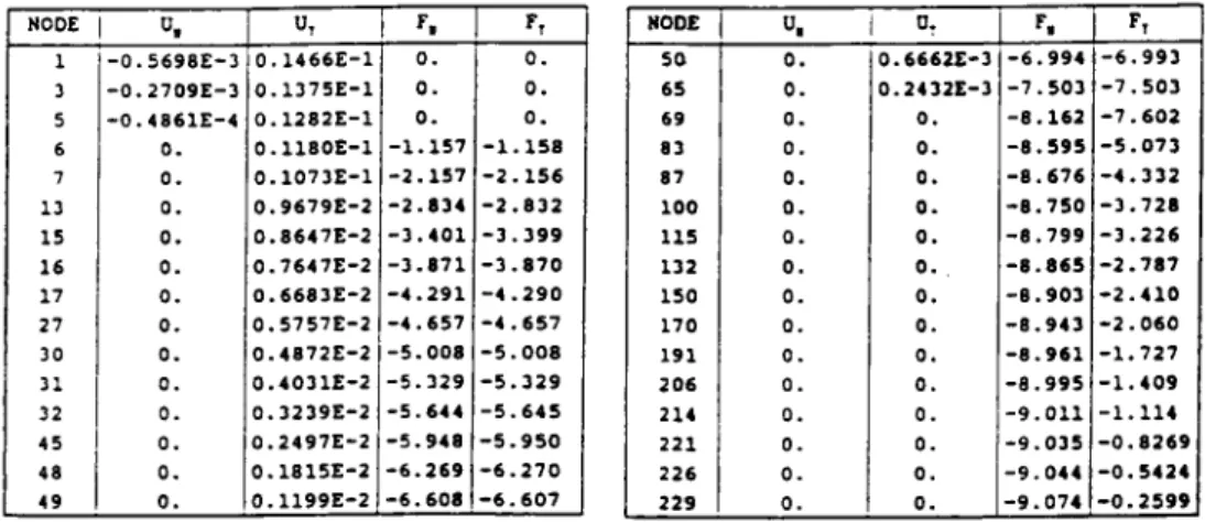
Table 2 : displacements and forces for the contact nodes case g-1 F-10 f--5
It can be observed on the table 2 that the relations (2) and (4)(5)(6) are verified with a very good accuracy.
M. RAOUS et ai.
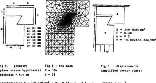
7.2. A dontall assembling (proposed by the CETIX-Paris).
This exaaple is a two body contact problem vith an oblique contact zone.
Flg.5. : geometry Fig.6 : the mésh Fig.7. : displacements
(plane stress hypothezis) N - 384 (muplified twenty times)
thickness - 6.4 ms K - 38
caracteristics E - 240 daN/ma: ; v - 0.38 : � - 0.2 ; �p - -.002656 daN/nm2
The nodal forces and the nodal d1splaceaents on the contact area for the corresponding nodas are given in the table 3.
Table 3 : solution on the contact area
The vertical displaceaents of the lover edge is -0.33m (variation between -0.327 and -0.329).
19 NUMERJCAL METHODS FOIt FRICTIONAL CONTACT
19
7.3. The punch problem vith loading and unloading
The specifications given by Curnier [321 «e used. This exemple has the advantage of
�ng 50.. analytieal mule* and usez londing history
including unlonding.
Fig.8. The mesh Fig.9. Loading évolution N-484 M-32
Elasticity under révolution symecry hypothosis E - 314 daN/a�,v-0, W - 0.4.
On the figures 10 and 11, the variations of F /u*F- along the radius of the punch are cted. The sliding zones are caracterized by the value 1 of this quotient. The other ts are sticked. On the figure 10, the comparison with a saut analytical solution gives
error of 71 : this ta due to the realrnass of the use of FI e lèsent for axisymmecrical blems. The figure 11 shows the solution after che unloading step. This complex solucion wing three différent zones (stick, invard-slip, outward-slip) has been reached with te che same number of itérations than the first one (sas table 4).
g.10. : lst step of the loading nunerical solution cheoretieal solution
(semi analytical)
Fig.ll. : 2nd step of the loading
M. RAOUS et al.
7.4. Structure assembling : bolted junction under intarnal pressure loading
This example deals with a real scale 80del on which experimental measurements have been done. This work has been supported by Technicatoue (Les Milles - France). It is a four body contact problem including three contact areas vith differenc friction coefficients. le is a three step londing : first the closure pressure is applied, then che pressure on the lover part and finally thé pressure on the upper part. The déplacement vith an amplicator coefficient of 100 are tiven on the folloving figures (elasticity under révolution symmetry hypothesis). N-674, !I-54.
Fig.12 closure pressure Fig.13. pressure on the Fig.14. pressure on the
lover part upper part
An identification of the différent friction coefficients has been done on the first loading step and the comparison botween the numerical results and expérimental datas for all the loading steps can be found in (29) and [30). The errors are less than 151 on the most significant quantities.
7.5. Friction modelling for metal forming processes
We focus on the behaviour of the sheet metal under the blankholder during che stamping process. This study has been supported by Regienov (Paris-France). It is a very chin structure with a large nuaber of contact nodes (N-784, M-251). Détails abouc the results can be found in [311. The folloving figure shows the évolution of the contact forces according to the inerease of the tangential displacement A applied to the righthand extremity. The extension of the sliding area can be observed along with the good vérification of Couloa�b's lav (Ft/� is alto plottad).
Fig.1S. contact forces evolution - normal force F, - tangential force F, --- quotient
Fr/W
21
NUNIERICAL METHODS FOR FRICT10NAL CONTACT
7.6. Cracked viscoplattic solid under alternative loading This exemple deals with the study of
the progression of a crack in a structure submicced to high variations of temperature. The contact betveen the edges of the crack is frictionless. The viscoplastie lav hau been given in paragraph 6 (relations (38)(39)).
Fig.16. the structure (the loading is harmonie)
Fi g. 17. displacement of a contact node Fig.lB.viscoplascic strain near the crack cip The unilatéral contact has been solved by the FPBC method described in paragraph 6.1 3 and the viscoplastic équations have been integrated by a Runge-Kutta method. Decails can be found in (20J.
8. COMPARATIVE COHPLTfAIIONAL TILLES
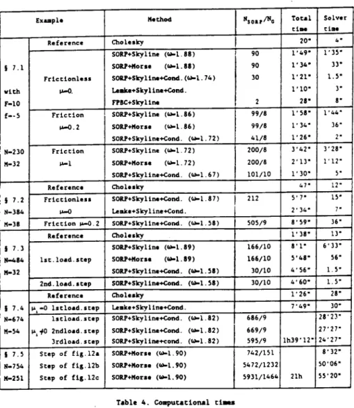
Computational times (on a Microvax II) corresponding to the examples referenced in paragraph 7 are presented in table 4. The methods are the ones presented in paragraph 6 either with a skyline storage or a liorse scorage (aparté �atrix scorage), with or without condensation. To give an idea of the cost of a contact problem. the computational time for a close clazzical elasticity problem on the same mesh is given as a 'reference' : the unilateral and friction conditions are replacad in this case by classical boundary conditions. The global number of iterations N,,,,is given together with the number N. of updating of Gk .
M. tuous et ai.
Table 4. Computational cimes
In conclusion, ve can note that it is important to have différent solvers to trest unilateral problems vith friction because the effieieney of each method depends on the nature of the problem. We can summarize this by a few reaarks.
For frictionless problème, the Lettke algoritha vith condensation and the FPBC seem to be the best ones.
Condensation is always suitable when the number !i of eontact nodes is small compared to the total number of nodes N. The only exception is vhen the finite élément macrix changes (in case of thermal effects for exemple) because in such a case the computacion of A« (see(48)) has to be done again and it vill be costly.
t�hen the number of contact nodes is large a Successive OverRelaxation method wich Projection using a sparze matrix scorage (Morse) is more adequace. The exemple 7.5 is pretty stiff because the solution includes a part of thé boundary vhere the contact is assoeiated to a very small compression force. Before convergence is reached the numerical
23
-
NUMERICAL METHODS FOR FRICT10NAL CONTACT
solution oscillantes betveen tvo states (un �', Fu -0 - · no contact) and (u,,-0. Fm-4« - � contact vith small compression) vhere t' and £« are cvo little négative quantities.
Condensation is very important for the multibody contact problems because the initial matrix is ill conditioned due to the connection relations betveen the différent solids which have been meshed separatively.
Actmowledgementt
Partial support for the developments described here has been provided by Tachnicatoue (Les !lilles-France) and Regienov (Rueil-Halmaison-Franee) which are gratefully acknowledged.
References :
111 Cottle R.Y., Cianessi F., Lions J.L. (editors) 'Varlational Inequalicies and Complementaricy Problems'. John Wlley, 1979.
(2] Duvaut C., Lions J.L,'Les inéquations en Mécanique et en Physique', Dunod Paris, 1972.
[3J Balinski M.L.. Cottle R.Y. ,'Complemeneariey and Fixed Point Problems' ,Mathernatica1 Programming Study. North Holland, 1978.
[4] Raous M., 'On cvo veriational inequalities arising from a periodie viscoeliscic unilatéral problem', in [11, ch.19, 285-302.
[5) Raous 1l., Latil J.C.,'Code d'éléments finis pour des problèmes de contact avec frottement formulés en termes d'inéquations variationnelles' ,in (24J, 259-278. [6) Bouc R., Geymonat G.. Jean li., Nayroles B., 'Cauchy and periodlc unilaeeral
problems for aging linear viscoelistic maeerials', J.Kath.Anal.App., il, n'1.7. 197"
�7J Panagiotopulos P.D., 'Inequalicy problems in Mechanics and Applications,, Sirkhaùser, Stuttgart, 1985.
[8J Fichera C., 'Boundary Value Problems of Elasticity Mien uniliteral Constrainrs' pp. 391-424, in Encyclopedia of Physics, VIa/2, Springer-Verlag, Berlin, 1972. 19) Stampacchia G.. 'On a problem of numerical analysis conneceed vich the cheory of
viriacional inequilicies'. Symposia Math, jsl, 281-293, 1972.
[10] Duvaut G., 'Equilibre d'un solide élastique avec contact unilatéral et frocremenc de Coulomb', CRAS, série A, 222. 263-265, 1980.
[11] Oden J.T., Pires E.B., 'Non local and nonlinear friction lavs and variational principles for contact problems in elaseiciey'. J.Appl.Mech. , 12, 1,67-76, 1983. [12] Cocu !!., 'Existence of solutions of Signorini's problem vith friction', Int. J.
Eng..Sci., 21. 5. 567-575, 1984.
(13) Raous M. , Pinto Y., *Direct and lcerative methods for cvo body contact problems', 547-550 in Proceed. 9th COBEK. Florianopolis, Brésil, 7-11 December 1986. !14) Raous li., 'A periodic problem in Viscoelasticity vich variable coefficients'
Int.J.Engn. Sci., 12. 1145-1168. 1981.
(151 Raous M.. 'Contacts unilatéraux avec frottement en viscoélasticité' , 269-297 in «Unilateral Problems in Structural Analysis", Publ. CISM n«288, Springer-Verlag Vienne, 1985.
[16J Raous M., 'Comportement d'un solide fissuré sous charges alternatives en visco- plasttcicE', J.Mec. Theor. Appl., n' spécial, 1984.
[17) Lemaitre J., Chaboche J.L, 'Mécanique des Matériaux', Dunod, Paris, 1985. [18) Chabrand P., 'Grandes variations de température pour des corps viscoélastiques'
Thème. Univ. de Provence, 1984.
!19j Chabrand P., Licht C., Maisonneuve o., Raous M., 'Residual Thermal Tempering 1
Scresses', to appear in 'Computer and Structures'.
M. RAOUS et al.
[20] Chabrand P.. Chazouane M. , 'Unilatéral problen for cracked viscoelastic or viscoplistic sollds', Proc. FEMCAD, Paris, 17-19 Octobre 1988.
[21] Latil J.C., 'Notice du code d'éléments finis PROTIS' , Note interne L11A n'2188 Marseille, France.
[221 Clowinski R., Lions J.L., Tréaoliires R., 'Anal/se numérique des Inéquations Var rationnelles ' , Dunod. Paris, 1976.
[231 Cryer C.41., 'The solution of a quadratlc programming problem using systemicic overrelaxacion', SIAM J. Control, 1, 385-392, 1971.
(24] Del Piero G., Maceri F. (editors). 'Unlliteral problem in Structural Analysis'. Ed. CISM,n' 304, Springer Verlag, Vienne, 1988.
[25] Klarbring A., 'Contact problems vith frictions by linear complementaricy'. 197-220, in [241.
[26] Barbosa H.J.C., Feijoo R.A., 'A numarical algoricha for Signorini's problem vith Coulomb frlction', 33-46, in [24].
[27J Pinto Y., Raous H., 'Direct nethe88ticel Programming method for che concacc belween two deformable solids', ICIAM-87, Paris, 29 Juin -3 Juillet 1987.
[28] Chabrand P., Raous 14., 'A model for opening and closing cracks in oligocyclic facigue',133-146, in Proc. SIBRAT-86, Salvador, Brésil. October 28-31, 1986. [29] Lebon F., Raous ti., boulègues D., 'Contact with friction modelling for the scudy
of a bolted junccion', 3-8, Vol.A, in Proc. S!lIRT-9, Lausanne (Suisse), 17-21 Aoûc 1987.
(30) Lebon F., Raous !!., 'Behavlour of a bolted junccion under internal pressure loading', 195-204, in Proc. NUCMAT 88, Nice (France), 22-24 Juin 1988.
[31] Chabrand P., Pinto Y., Raous li., 'Numerlcal modelling of friction for metal forming processes',93-99, in Proc. Euromech 223 : 'ltodelling of metal forming processes' Sophia-Antipolis, France, 29-31 Août 1988.
[32] Curnier A., Alart P., 'A generalized Newton liethod for contact problems vich friction', in this Journal.
[33] Barbosa H., Raous M.. Aitken accoloratlon for fricrional concact algorichms. in preparation.
25
III - OPTIONS DE PRISE EN COMPTE DES DONNEES
La description des conditions aux limites de type Dirich-
let fait appel au module COBDC1 et conduit à une S.D. BDCL,
mais à l'intérieur d'un module de traitement particulier de nom
CONSBL.
La caractérisation du contact/frottement est le travail
d'un module de nom CONFRO dont le résultat du travail est une
S.D. nouvelle : CTFR.
Enfin, la description des chargements surfaciques se fait
par l'intermédiaire du module ELAST et conduit à une S.D. B,
mais à l'intérieur d'un module de traitement particulier de nom
COSECM.
Comme on le verra ci-après, un noeud de contact appartient à
une portion de frontière dite de contact et est affecté de la
référence de cette portion de frontière. Il est traité dans son
repère local (normale,tangente), où la normale est la normale
extérieure à la frontière en ce noeud.
Pour chaque noeud de contact, il y a donc changement de
base, du repère global (x,y) au repère local (n,'t). I1 arrive
souvent qu'un noeud référencé de contact (bord de la portion de
frontière de cette référence) ait sa composante normale de con-
tact et sa composante tangentielle, non pas de frottement, mais
bloquée en conditions aux limites ou bien chargée par une force
nodale. Ceci nécessite que l'on admette des "dérogations" au
principe qui veut qu'une référence corresponde à une fonction
unique et c'est ce qui motive le traitement particulier des
descriptions de conditions aux limites ou de chargements, le-
quel particularisme étant, comme on le verra, fort peu impor-
tant du point de vue de l'utilisateur.
Spécificités des données relatives au contact et frottement :
Tout au long de la procédure éléments finis, un noeud décla-
ré de contact est donc traité dans son repère local (n,t). On
est notamment amené, en cours de résolution, à contrôler son
déplacement normal un n et sa force tangentielle Ft (seuil de glissement). La caractéristique prise en compte au niveau des données est l'angle (0�,�) entre l'axe global des x et la nor- male à la frontière. Il s'ensuit qu'un certain nombre de noeuds de contact (et bien souvent tous...), présentant le même angle
Au niveau du maillage, on admet de donner le même numéro
de référence à tous les noeuds de contact présentant le même
angle (Ôx,n) : ceci caractérise une portion de frontière de
contact. A ce principe, cependant, deux restrictions :
- si on traite d'une
portion de frontière parfaitement
courbe (mais la discrétisation est en PI droits...),
alors chaque noeud de contact constitue en lui même une
portion de frontière de contact. C'est un cas théorique
non validé.
- si le problème admet du frottement, le coefficient de
frottement doit être le même pour tous les noeuds d'une
même portion de frontière de contact avec frottement. Si
tel n'était pas le cas, il y aurait lieu de donner la
priorité à la valeur uniforme du coefficient de frotte-
ment par rapport à la valeur uniforme des angles (Ox,n),
c'est à dire de distinguer plusieurs portions de fron-
tière ayant le même angle (Ox,n).
La formulation d'un problème de condition unilatérale
conduit à imposer des déplacements normaux un � 0. Le traite-
ment standard doit donc ne prendre en compte que des déplace-
ments nuls (contact sur l'obstacle) ou négatifs (décollement de
l'obstacle). On admet cependant ici la possibilité de prendre
en compte des déplacements un � 0. , dans une limite acceptable
ce qui, d'une certaine façon, assimile le problème de contact à
un problème de conditions aux limites décrites par déplacements
imposés non nuls (aussi bien négatifs, d'ailleurs).
Ceci permet de traiter des cas de contact sur un obstacle
fixe non uniforme, "en escalier" par exemple, vis a vis d'une
portion de frontière de contact déterminée. C'est pourquoi les
données comportent la définition des valeurs des un n admis par
portion de frontière de contact et offrent la possibilité de
décrire un certain nombre de un différents pour une portion de
27
IV - MODULE INTERACTIF GYPTXX
Le module interactif GYPTXX a pour but essentiel de cons-
tituer le fichier de données nécessaire à la résolution d'un
problème de contact. Il permet également d'effectuer cette ré-
solution en interactif, avec sortie des résultats sur écran,
conformément au fonctionnement habituel des modules interactifs
de MODULEF. Il semble cependant plus sage, sauf pour des tests
de peu d'envergure, de faire exécuter ensuite GYPTIS dans la
file des traitements par lots.
L'utilisation de GYPTXX ne demande que peu de connaissan-
ce des spécificités de GYPTIS, car il pose des questions aussi
courtes et claires que possible. En cas d'hésitation, l'utili-
sateur peut toujours répondre par un point d'interrogation (?),
ce qui entraine la production d'une explication détaillée,
après quoi la question est à nouveau posée. Une erreur de type
Fortran de donnée entraine seulement une demande de reformula-
V - MODULE GYPTIS : MISE EN OEUVRE
Pour résoudre un problème de contact avec frottement dé-
terminé, l'utilisation de GYPTIS suppose :
- d'avoir réalisé le
maillage :
le pas ( distance entre deux noeuds consécutifs ) doit
être constant pour les noeuds de contact, faute de quoi
les calculs de forces normales et tangentielles à la so-
lution seraient erronés,
- d'avoir constitué le fichier de données correspondant,
en faisant appel au module GYPTXX,
- d'attacher au travail :
- le fichier de données, à l'étiquette logique prévue à
cet effet,
- le fichier imprimante, à l'étiquette logique prévue à
cet effet,
- éventuellement ( problème à symétrie de révolution,
éléments TRIA AP1D au lieu de TRIA 2P1D ), le fichier
POBA à l'étiauette logique 1,
- de lancer l'éxécution.
Par principe, GYPTIS n'admet l'existence que de la S.D.
NOPO du maillage du domaine. Il construit toutes les autres
S.D. dont il a besoin et, à la fin, les détruit sauf si on a
manifesté la volonté de les conserver ( logique SERVAR, en don-
nées ). Bien entendu, la S.D. B contenant les déplacements et
la S.D. TAE des contraintes, utilisables pour l'exploitation
29
VI - DESCRIPTION DETAILLEE DES DONNEES
Données générales :
-1 Si l'on ne travaille pas en interactif, aller à (1)
0 NODATA (78 caractères)
Nom du fichier des données, question posée à
l'écran.
1 TITRE (80 caractères)
Titre donné au travail.
2 IMPRE (entier � 0)
Niveau de bavardage, correspondant aux conven-
tions MODULEF. En séquence de mise au point, on
peut donner :
IMPRE = 11 , ce qui permet d'avoir une trace de
chaque manipulation de S.D.,
IMPRE = 12 , ce qui fournit en plus le contenu
du tableau de sauvegarde du commun
pour chaque S.D. manipulée.
3 NOMGEN (6 caractères)
Nom générique qui permet de déterminer les noms
de tous les fichiers des S.D. traitées, sauf la
S.D. NOPO. Principe : pour la S.D. TOTO, on au-
ra un nom de fichier : NOMGEN//'TOTO.DAT'.
4 SERVAR (logique)
Vrai si l'on désire conserver toutes les S.D.
créées par le travail. Sinon, une fois le tra-
vail fini, ne subsisteront que :
- la S.D. NOPO du maillage,
- la S.D. B des déplacements solutions
(NOMGEN//'BS.DAT')
- la S.D. TAE des contraintes à la solution
(NOMGEN//'TAES.DAT')
5 NOM NOPO (72 caractères)
Nom du fichier de la S.D. NOPO du maillage.
6 AXISYM (logique)
Vrai si l'on traite un problème à symétrie de
Description des conditions aux limites :
7 NBRFX (entier)
Nombre de numéros de référence décrivant les
blocages en x.
8 NBRFY (entier)
Nombre de numéros de référence décrivant les
blocages en y.
9 Si NBRFX 4 0 , aller à (11)
10 (NREFX(I),I=1.NBRFX) (tableau entier)
Liste des NBRFX numéros de référence décrivant
les blocages en x.
11 Si NBRFY 5 0 , aller à (13)
12 (NREFY(I),I=1,NBRFY) (tableau entier)
Liste des NBRFY numéros de référence décrivant
les blocages en y.
13 CLIMNN (logique)
Vrai si :
- on admet des déplacements non nuls imposés
par numéros de référence,
- on définit ( ou redéfinit ) isolément les
conditions aux limites de certains noeuds
frontaliers.
14 Si CLIMNN est faux, aller à (21)
15 NBCLRF (entier)
Nombre de numéros de référence pour lesquels on
impose des déplacements non nuls.
16 Si NBCLRF � 0 , aller à (18)
17 Boucle sur I = 1, NBCLRF :
NUREF(I) (entier) : I-ième de ces numéros de
référence.
VBNNR(1,I) (réel s.-p.) : son déplacement imposé
en x (*) .
VBNNR(2.I) (réel s.-p.) : son déplacement imposé
en y (*). Fin de boucle
(*) Si l'un des déplacements imposés n'a pas de sens
( équation libre ou bien déplacement déjà correc-
tement défini ), lui attribuer ici une valeur :
ui � l.E+15.
18 NBNDBL (entier)
Nombre de noeuds de conditions aux limites dont
les blocages sont décrits isolément (hors réfé-