Modeling and Simulation of an Aircraft Environmental Control System

(1)

UNIVERSITÉ DE MONTRÉAL

MODELING AND SIMULATION OF AN AIRCRAFT ENVIRONMENTAL CONTROL SYSTEM

DANIEL PEREZ LINARES

DÉPARTEMENT DE GÉNIE CHIMIQUE ÉCOLE POLYTECHNIQUE DE MONTRÉAL

MÉMOIRE PRÉSENTÉ EN VUE DE L’OBTENTION DU DIPLÔME DE MAÎTRISE ÈS SCIENCES APPLIQUÉES

(GÉNIE CHIMIQUE) AOÛT 2016

(2)

UNIVERSITÉ DE MONTRÉAL

ÉCOLE POLYTECHNIQUE DE MONTRÉAL

Ce mémoire intitulé :

MODELING AND SIMULATION OF AN AIRCRAFT ENVIRONMENTAL CONTROL SYSTEM

présenté par : PEREZ LINARES Daniel

en vue de l’obtention du diplôme de : Maîtrise ès sciences appliquées a été dûment accepté par le jury d’examen constitué de :

M. PERRIER Michel, Ph. D, président

M. SRINIVASAN Bala, Ph. D., membre et directeur de recherche M. BEAULAC Sébastien, membre

(3)

DEDICATION

(4)

ACKNOWLEDGEMENTS

Je tiens à remercier tout d’abord mon directeur Bala Srinivasan pour la confiance qu’il m’a accordée durant ce projet. Ses conseils m’ont beaucoup guidé et son support m’a encouragé dans les moments les plus difficiles. J’en suis grandement reconnaissant.

Merci à mes collègues chez Bombardier : Amir, Pascal, Yannick, André, Hongzhi, Tariq, Benoit, Amine, Walid et Sébastien. Par votre présence, vous avez rendu mon projet des plus agréables. Merci de m’avoir initié à Clash of Clans auquel je joue toujours d’ailleurs.

Merci à mes amis colocataires qui m’ont encouragé lorsque la motivation n’était pas au rendez-vous. Merci pour les bons moments passés ensemble.

Finalement, je tiens à remercier ma famille et proches pour toujours avoir été là pour moi, je vous en suis très reconnaissant.

(5)

RÉSUMÉ

Dans ce mémoire, on traite de la modélisation du Système de contrôle de l’environnement (SCE) des avions CS300 de Bombardier en se basant sur des données de vol et des modèles analytiques. Plus précisément, les données de vol et l’analyse dimensionnelle sont utilisées pour créer des modèles des composantes du SCE. La principale fonctionnalité du SCE est de fournir les conditions optimales dans les cabines afin d’assurer le confort des passagers. Ainsi, ce système assure une pressurisation convenable, régule la température et fournit une ventilation adéquate en fonction du nombre de passagers en traitant l’air provenant des moteurs à réaction. Les composantes principales du SCE comprennent quatre échangeurs de chaleur à plaques et ailettes, un ventilateur, un compresseur, une turbine, des vannes de régulation, des sources et des puits de chaleur, et les conduites faisant circuler l’air. Pour chaque composante mécanique, les paramètres de performance ont été adimentionnalisés et cartographiés. Lorsque des surfaces tridimensionnelles étaient requises, les paramètres de performances issus des données de vol ont été complémentés avec des hypothèse de lissage de surface. En procédant de cette façon, un problème de régularisation a pu être résolu. L’architecture du SCE a été créée et résolu à l’aide du logiciel Flowmaster® (FM). En effet, le logiciel permet d’intégrer des scripts personnalisés au modèle ce qui le rend très flexible. Les résultats de simulation du modèle ont été comparés aux données de vol et les deux convergent vers des valeurs similaires. Seuls les résultats de simulation des cas avec beaucoup d’humidité (HD et XHD) n’ont pas convergé vers les températures attendues parce que le calcul de transfert thermique dans Flowmaster néglige la chaleur latente de l’eau. Néanmoins, un algorithme Matlab est suggéré dans ce mémoire afin d’améliorer celle du logiciel. Pour tous les autres cas de vol (XCD, CD et ISA), le modèle est capable de prédire les conditions dans les cabines selon l’altitude, la température extérieure, et la vitesse de l’avion.

(6)

ABSTRACT

In this memoir we address the task of modeling Bombardier’s CSeries 300 aircraft environmental control system (ECS) based on flight data. That is, flight data and dimensional analysis is used to model the system main components. The function of the ECS is to supply optimal cabin conditions to the passengers’ cabin (ventilation, pressurization, temperature control and best possible humidity) using bleed air coming from the engines. The system components comprise four heat exchangers, a fan, a compressor, a turbine, control valves, cabin heat sources and sinks and the interconnecting piping. For each component analogous to a mechanical machine, the performance parameters were adimensionalized and their respective performance maps were built. When tridimensional reliable maps were required, flight data was augmented with smoothing assumptions. By doing so, a regularized optimization problem could be solved. The ECS network was built and solved with Flowmaster® software (FM). In fact, the software allows for customized scripts and performance maps to be easily imported to the model. The simulation of the final model was compared with flight data and converged to very similar results. Only simulations with very high humidity (HD and XHD cases) failed to converge to the expected temperature because Flowmaster’s heat exchanger calculation neglected water latent heat. Nevertheless, code is suggested in this work to improve the software calculation method. For all the other cases (XCD, CD and ISA), the model is able to predict cabin conditions at any permitted altitude and aircraft speed. Moreover, the model and can be used as a design tool or analysis tool within Bombardier’s support team.

(7)

LIST OF TABLES

Table 1 Pressure drop Input data ... 14

Table 2 Pressure drop Output Values ... 14

Table 3 Heat-Exchanger Input data ... 20

Table 4 Hot stream outputs ... 20

Table 5 Cold stream outputs ... 21

Table 6 Fan Reference data ... 26

Table 7 Fan Inlet conditions ... 27

Table 8 Fan Efficiency and actual pressure increase ... 27

Table 9 Fan Output values ... 27

Table 10 Compressor Input values ... 35

Table 11 Compressor Output values ... 35

Table 12 Turbine Input values... 39

Table 13 Turbine Output values ... 39

Table 14 Cd valve Inputs values ... 41

Table 15 Cd valve Output values ... 42

Table 16 Controller components ... 43

Table 17 Ambient temperature and humidity [6] ... 49

Table 18 Atmospheric pressure law [37] ... 50

Table 19 Cabin pressure law [6] ... 51

Table 20 Dual pack fcv flow schedule [6] ... 52

Table 21 Single pack fcv flow schedule [6] ... 52

Table 22 Cabin flow split [6] ... 54

(11)

Table 24 Number of cabin passengers ... 57

Table 25 Cockpit effective area ... 59

Table 26 Aft cabin effective area ... 59

Table 27 CS300 UA factors ... 60

Table 28 Thermal loss coefficients ... 60

Table 29 Ram outlet pressure coefficients ... 65

Table 30 Valve pressure loss coefficients ... 66

Table 31 Cockpit fixed heat loads ... 67

Table 32 Electrical + IFE heat loads ... 67

Table 33 Floor heat flow ... 68

Table 34 External input summary ... 70

Table 35 OAT input values ... 73

Table 36 flight case identification ... 74

Table 37 Turbine data excluded ... 84

Table 38 Flight cases tested ... 97

Table 39 Output parameters compared ... 98

Table 40 Simulation input values ... 100

Table 41 Steady-state simulation results ... 102

Table 42 Expected Simulation results (reference) ... 103

Table 43 Absolute deviations from expected values ... 104

Table 44 Water condensation assessment ... 106

Table 45 Heat-exchanger calculation improvement inputs ... 111

(12)

LIST OF FIGURES

Figure 1 Simplified ECS block diagram ... 4

Figure 2 Ecs schematic [6] ... 6

Figure 3 Right and left packs [7] ... 7

Figure 4 Cabin Control ... 8

Figure 5 Error in flow rate prediction for a single pipe due to using incompressible flow assumptions [18] ... 10

Figure 6 Pipe component ... 11

Figure 7 Curve pressure loss component ... 14

Figure 8 Heat-exchanger component ... 15

Figure 9 heater-cooler component ... 19

Figure 10 Fan dimensionless groups [29] ... 23

Figure 11 Fan component ... 24

Figure 12 Fan polytropic efficiency plot ... 25

Figure 13 Fan pressure increase plot ... 26

Figure 14 Compressor component ... 28

Figure 15 Typical compressor performance map [35] ... 33

Figure 16 Compressor pressure ratio surface ... 34

Figure 17 Compressor efficiency surface ... 34

Figure 18 Turbine component ... 36

Figure 19 Typical Turbine map ... 38

Figure 20 Turbine cmfr vs pr ... 38

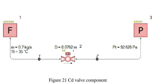
Figure 21 Cd valve component ... 40

(13)

Figure 23 Flowmaster ECS pack model schematic ... 45

Figure 24 Flowmaster distribution model schematic ... 48

Figure 25 Outlet coefficient of discharge plot... 54

Figure 26 ACM matching algorithm ... 55

Figure 27 Mechanical loss vs rotational speed plot ... 56

Figure 28 Solar radiation intensity plot ... 58

Figure 29 Inside view of shx and phx ... 61

Figure 30 SHX inlet dimensions (ram air side) ... 62

Figure 31 FM’s external inputs tab ... 63

Figure 32 Ram air recovery factor for different altitudes and speeds [6] ... 64

Figure 33 Pressure coefficient vs. flow coefficient ... 76

Figure 34 Efficiency vs. flow coefficient ... 76

Figure 35 Fan pressure increase vs. flow chart ... 78

Figure 36 Fan polytropic efficiency vs. flow chart ... 78

Figure 37 Pressure ratio and efficiency data points ... 82

Figure 38 Compressor performance surfaces ... 83

Figure 39 Turbine cmfr vs. pr plot ... 85

Figure 40 Turbine performance surfaces ... 86

Figure 41 PHX performance map ... 88

Figure 42 PHX pressure loss map (hot stream) ... 89

Figure 43 PHX pressure drop map (cold stream) ... 89

Figure 44 SHX performance map ... 90

Figure 45 SHX pressure loss map (hot stream) ... 91

(14)

Figure 47 REH performance capability chart ... 92

Figure 48 REH performance map ... 93

Figure 49 REH pressure loss map (hot stream) ... 94

Figure 50 REH pressure loss map (cold stream) ... 94

Figure 51 COND performance map ... 95

Figure 52 COND pressure loss map (hot stream) ... 96

Figure 53 COND pressure loss map (cold stream) ... 96

Figure 54 APU8ISA2P ram air data ... 108

(15)

LIST OF SYMBOLS AND ABBREVIATIONS

Acronyms

A/C Aircraft

ACM Air Cycle Machine

ACU Air Conditioning Unit

APU Auxiliary Power Unit

BA Bombardier Aerospace

CD Cold Day conditions

Cd Coefficient of discharge

CDS Condenser

CDTS Compressor Discharge Temperature Sensor

CMFR Corrected Mass Flow Rate

CS Corrected Speed

DART Dry Air Rated Temperature

DBT Dry Bulb Temperature

DTS Duct Temperature Sensor

ECS Environmental Control System

EOS Equation of State

FCV Flow Control Valve

FSV Flow Sensor Venturi

FWD Forward Part of Cabin

GND Ground

HAAO High Altitude Airport Operation

HD Hot Day conditions

HX Heat Exchanger

IAMS Integrated Air Management System

IASC Integrated Air System Controller

ITD Inlet Temperature Difference

LPDS Low Pressure Distribution System

(16)

LTS Liebherr Aerospace Toulouse S.A.S

MFR Mass Flow Rate

MHX Main Heat Exchanger (same as SHX)

MIXTS Mix manifold Temperature Sensor

NTU Number of Transfer Units

OAT Outside Ambient Temperature

OFV Outflow Valve

PAX Passengers

PDTS Pack Discharge Temperature Sensor

PHX Primary Heat Exchanger

PR Pressure Ratio

PRSOV Pressure Regulating and Shut-Off Valve

PTS Pack Temperature Sensor

RARV Ram Air Regulating Valve

REH Reheater

SHX Secondary Heat Exchanger

TACKV Trim Air Check Valve

TAV Trim Air Valve

TAPRV Trim Air Pressure Regulating Valve

TCV Temperature Control Valve

VENTS Ventilated Temperature Sensor

WE Water Extractor

Symbols

A Area

Cp Specific heat capacity at constant pressure

𝐶_𝑟 Ratio of capacity coefficients

D Diameter

ℎ Specific enthalpy

M Mach number

(17)

N Rotational speed

P Pressure

𝑄̇ Volumetric flow rate

𝑄̇ Heat flow

R Specific gas constant

T Temperature

U Overall heat transfer coefficient

V Velocity

W Power

Z Compressibility factor

Z Fan correction factor

𝛼 Speed of sound

𝜌 Density

𝛾 Heat capacity ratio of air

Subscripts

0 Total or stagnation condition

1 Inlet

2 Outlet

ise Isentropic

(18)

LIST OF APPENDICES

(19)

CHAPTER 1 INTRODUCTION

1.1 Problematic and hypothesis

Simulation-based engineering (SBE) focuses on the computational tools and techniques to evaluate performance parameters of complex systems and has become the primary means of analysis in the industry. The advantages of SBE are numerous: minimal time spent on analysis, reduced costs, and less planning and logistics compared to bench-testing. Ultimately, it improves decision-making among designers and engineers. For example, in the automotive industry, crash worthiness analysis allows engineers to predict the effects of a car crash on the vehicle body by means of computer simulation. This is a major improvement in the automobile design process since, previously, the vehicle had to be crashed in a controlled environment in the real world, which can be expensive and requires considerable planning.

Aircraft simulation modeling consists on creating a digital prototype of a given system in order to predict and evaluate its performance. When such models attain a certain level of maturity, they can become a design tool. The model can be used to discard poor designs early during the design process and achieve significant customer satisfaction.

One of the main concerns in commercial aircraft design is to achieve passenger comfort during flight by providing adequate ventilation, temperature control and pressurization. The system responsible of providing these optimal cabin conditions is called the Environmental Control System (ECS). During a typical flight where ambient conditions change tremendously (altitude, ambient temperature, aircraft speed), this system is to supply adequate heating or cooling to the cabin in the most efficient manner.

Currently, Bombardier’s aircraft ECSs are designed by third parties. Thus, thermodynamic analysis with regard to the ECS relies greatly on data not readily available by Bombardier. Moreover, no in-house ECS model is available to predict cabin conditions for every flight case. However, data consisting on 236 different flight cases provided by CS100/300 ECS manufacturer is available. The data comprise Auxiliary Power Unit (APU), one engine and two engines cases ground or in-flight under various ambient conditions. For each case, data on the inlet and outlet conditions (mass

(20)

flow rate, temperature, pressure) and efficiencies (if applicable) of the main components of the ECS are given.

Given this amount of information, it was postulated that an ECS model could be reverse engineered by modeling each main component and connecting them. Consequently, the motivation on developing an ECS model to predict cabin conditions ensued.

1.2 Objectives

In light of what’s been previously mentioned, the general objective of this thesis is to:

1. Develop a model of the environmental control system based on analytical models that are derived from physical principles, conservation laws for instance, and data-based models obtained from flight-testing. Use Flowmaster software to build the model.

2. Predict temperature and pressure at various points of the system under different flight conditions with a reasonable accuracy.

The sub-objectives can be detailed as follows:

1. Verification of each component presented in the schematic of the ECS. 2. Validation of the model by comparing with data.

1.3 Methodology and organisation

Flowmaster software is used to model the system. The choice of this modeling tool was made prior to the beginning of this project. Nevertheless, one of the reasons for choosing this platform is based on its modular approach in opposition to written code. In fact, the ECS components can be connected to each other in a very intuitive and user-friendly manner. Moreover, the model can be understood more easily by other people without the considerable effort in decrypting lines of code. In theory, highly accurate modeling of components such as pipes and heat-exchangers could be undertaken by considering two-dimensional or three-dimensional flow, but the data available to us assumes the flow is directed to only one direction, i.e. the direction of the flow. Thus, in this work

(21)

the ECS is considered as a 1D thermo-fluid system that could be solved in principle with Flowmaster, a 1D thermo-fluid software.

This master’s thesis is divided in 5 chapters. Chapter 2 presents the state of the art with regards to ECS modeling. A review of literature is reported and the governing equations of the main components of the ECS model are introduced.

In Chapter 3, the developed model is presented by describing its internal and external inputs. In the chapter afterward, the performance maps obtained and simulation results are stated. Finally, in chapter 5, discussion with regard to the results is presented.

(22)

CHAPTER 2 STATE OF THE ART

2.1 Environmental control system description

Many aircraft systems carry different functions to ensure safe flight. To name some examples we can think of propulsion, avionics, fuel, landing gear, auxiliary power unit (APU) and pneumatics. The Environmental Control System (ECS) is another example of great importance. In this section, we will describe its function, explain what its components are and how it works.

The main function of the Environmental Control System is to provide the conditions for comfortable travelling of passengers. This includes optimum cabin air pressure, cooling, heating and ventilation within the passengers’ cabin compartment, cockpit and cargo compartments. [1] The technology of an ECS is based on air-cycle refrigeration process. Such process is called the reversed Brayton cycle. [2] Although, it is important to remember that an ECS is not a closed system as the Brayton cycle, but is often considered as so in thermodynamic analysis.

In Figure 1, the ECS is schematically represented by the Engine Bleed Air System, the Air Conditioning System andthe cabins and cockpit. Air is first extracted from the engine or APU and flows to the Wing Anti-ice system (WAIS) and Air conditioning system. The air conditioning system is composed of many units processing hot and pressurized bleed air. Here, air is ultimately cooled down and expanded down to a pressure around 1 atm. Thereafter, the breathable gas is sent

Figure 1 Simplified ECS block diagram Engine

Bleed Air

Cabins and Cockpit Ram air intake

Air Conditioning

Air from Engine Air

exhaust Ram air discharge

(23)

to passenger cabins, cockpit and cargo compartments. Approximately, one half of the amount of air sent to cabins is recycled while the other half is exhausted to the ambient. [3]

Air conditioning system

Air entering the air conditioning system comes from the engine bleed. The first unit the air encounters is the primary heat-exchanger where heat is removed with ambient air (ram air) as the coolant fluid. Next, air pressure is increased by a centrifugal compressor, part of the Air Cycle Machine (ACM). Since this step increases the temperature, air is passed through a secondary heat-exchanger. Air is cooled in the primary heat-exchanger prior to being compressed because the amount of work required to compress a gas decreases as the temperature of the gas decreases. [4] After passing through the secondary heat-exchanger, air flows through two other heat-exchangers: the reheater and condenser. In the reheater, a small amount of heat is transferred to the cold fluid. In the condenser, air is cooled as much as possible so as to condense the water vapor that air might carry. The condensed water is then removed by the water extractor. Removal of water is very important in order to avoid icing that can break the turbine. It also enables the turbine outlet temperature to reach sub-zero state. [4]

At this point, air is very cold so it is warmed in the reheater (in case some icing has formed) prior to be expanded in the turbine. At the turbine exit, air might be below the target temperature. Therefore, it is heated with a small amount of conditioned hot engine bleed air. The non-conditioned flow is controlled by the Temperature Control Valve (TCV) coupled to the Integrated Air System Controller (IASC). The last unit is the mix manifold where air is mixed with recycled cabin air. As a matter of fact, without recirculation, a greater fuel penalty on the aircraft would be imposed. [5]

The central component of the air conditioning system is the three-wheel ACM unit comprising the turbine, compressor and fan mounted on the same shaft. [3] It is the power output from the turbine that drives the compressor and fan. The fan is located in the ram air channel and its purpose is to ensure there is sufficient flow in the channel when aircraft is on ground. Because of space and weight constraints imposed in new generation aircrafts, the rotating elements in the ACM are very small. As a result, ACMs must handle significant air mass flows with large enthalpy drops. These constraints can be achieved with high rotational speeds ranging from 60 000 to 90 000 RPM.

(24)

Note that since there are two engines in the CSeries aircrafts, there are two identical packs, each containing one ACM and all the other components described previously. The left pack is supplied with air from the left engine and the other from the right engine. The mix manifold mixes air coming from both packs in addition to the recycled cabin air. Figure 2 illustrates the ECS flow diagram, while Figure 3 shows the equivalent Catia drawing of the left and right packs.

(25)

Figure 3 Right and left packs [7]

Integrated air management system

Flow control within the packs and cabins is monitored by the Integrated Air Management System (IAMS). Flow is controlled by action of the Flow Control Valve (FCV) and will depend on the flow schedule, which in turn depends on flight conditions such as the altitude, number of passengers, number of packs available, cargo heating, etc.

Temperature is also monitored by the IAMS. For this task, temperature sensors are installed at specific locations in the cabin, cockpit, packs and ducts. The ECS temperature readings are regulated by action of three valves: TAV, TCV and RARV. For example, the temperature at the Compressor Discharge Temperature Sensor (CDTS) must be kept at 148°C when possible. When the temperature is higher, the RARV position is changed to keep the temperature at its target value. However, RARV action is limited. If the temperature cannot be regulated and exceeds 220°C, then the flow through the pack is reduced by action of the FCV. As last resort, if the temperature goes above 232°C, the FCV is completely closed and the pack is turned down. [6] Clearly, every control action described so far is performed automatically by the IAMS reducing the pilot load tremendously.

(26)

Another example of temperature control performed by action of the TCV can be found at the outlet of the water extractor. In fact, the temperature at this location is measured by the Pack Temperature Sensor (PTS) and must not go below a limit to avoid freezing. This temperature limit depends on the aircraft altitude and it is programmed in the IASC. [6]

Low pressure distribution system

The LPDS consists of all the ducts and control valves used to regulate pressure inside the cabin downstream of the mix manifold. The cabin pressure is controlled by modulating pressure drop at the outflow valve (OFV). In addition, positive pressure relief valves prevent over-pressurizing the passengers’ cabin.

Dynamic control of ECS

Control of the most important cabin parameters, pressure and temperature, is carried out by manipulation of the outflow valve (OFV) and TCV, respectively. For temperature control, it might also be necessary to open one of the three trim air valves (TAVs) if TCV action is not sufficient. Figure 4 illustrates cabin control inputs and outputs. Note that humidity is not a controlled parameter but rather a passive parameter.

(27)

2.2 Review of literature

Experimental study of aircraft ECS performance have been undertaken by Zhao et al. [2] during off-design conditions and the system response by changing bleed air flow rate and altitude was investigated.

With regard to ECS modeling, one of the first ECS models mentioned in literature dates back to 1975. Eichler [8] developed dynamic models for each component and studied the stability of the whole system. However, the mathematical base of such component models are undescribed. Thus, one can hardly assess the validity of his results. Moreover, time constants were held constant although these happen to be function of flow rate.

Santos, Andrade and Zaparoli [1, 9] developed an air-cycle machine model to simulate the effects of changing Mach number, cabin altitude and cabin recirculation air. However, their model assumed constant efficiencies with regard to the main components (heat-exchangers effectiveness, compressor and turbine efficiencies), whereas these are function of multiple parameters.

More recently, Lin and Tu [10, 11] integrated cabin temperature control based on Fuzzy method to a dynamic ECS model. Furthermore, their heat exchanger is more elaborated as it is a two-dimensional transient model. In order to derive such model, they used a discretized lumped parameter method where heat and mass transfer phenomena were simplified by assuming the Lewis number was equal to one.

On a more specific level, Vargas and Bejan [12-14] have been conducted research on heat-exchanger optimization. They advanced a method for optimal sizing of ECS cross flow heat exchangers by minimisation of ACM entropy generation. Their heat-exchanger model consisted of a specific well-known effectiveness-NTU relation. Perez-Grande and Leo [15] accomplished a similar study by considering two optimum functions: the entropy generation and heat-exchanger weight.

Comini et al. [16, 17] have addressed the heat and mass transfer description in air-cooling applications where latent (condensation and evaporation) and sensible heat transfer is involved. Their analysis can be used to develop more accurate geometrical heat-exchanger models, as it is a three-dimensional approach. Nevertheless, they assumed heat and mass transfer analogy for simplification and their description only applies to laminar flow.

(28)

2.3 Mathematical background

In this section, the mathematical model of each ECS component is presented. An assessment is also performed to validate Flowmaster software by comparing FM’s results to hand calculations. This step will help the reader get familiar with the way FM solves systems that are more complex and verify that the solution is in agreement with theory.

2.3.1 Pressure drop model

Figure 5 Error in flow rate prediction for a single pipe due to using incompressible flow assumptions [18]

Designing gas-piping networks requires mathematical models that address all the relevant phenomena like sonic choking, accurate pressure drop and psychrometrics. Compressible flow simulation takes into account all of these phenomena whereas incompressible simulations cannot predict choking and are inherently inaccurate with respect to flow rate or pressure drop prediction. Figure 5 illustrate the incompressible flow rate error for different fL/D (Equation 10) ratios as a function of pressure drop over inlet pressure ratio (PR). Therefore, a compressible model is preferred for ECS modeling.

(29)

The drawback of compressible flow modeling is that it is a challenging technical application because of the couple nature of the governing equations. When a real gas model is included, the complications compound even further. However, FM software can accurately calculate pressure drop, flow rates and temperatures in gas systems by solving the coupled governing equations simultaneously.

The Cylindrical gas pipe component as shown in Figure 6 is used to model pressure drop in cylindrical pipes. Friction, heat transfer and variation in cross sectional area affect the flow of a compressible fluid in pipes. Nevertheless, only the adiabatic, constant cross section area with friction is analyzed here, as this is the most common occurrence for ECS piping.

Pipes and ducts

Figure 6 Pipe component

The equations governing steady-state compressible fluids flow in pipes are derived from mass, momentum and energy balance [19]. An equation of state (EOS) that relates gas intensive properties as well as the second law are also required. [20]

𝑴𝒂𝒔𝒔 𝒃𝒂𝒍𝒂𝒏𝒄𝒆: 𝒅𝝆_𝝆 +𝒅𝑽_𝑽 = 𝟎 (1)

𝑴𝒐𝒎𝒆𝒎𝒕𝒖𝒎: 𝒅𝑷 +𝟏_𝟐𝝆𝑽𝟐 𝒇_𝑫𝒅𝒙 + 𝝆𝑽𝒅𝑽 + 𝝆𝒈𝒅𝒛 = 𝟎 (2)

𝑭𝒊𝒓𝒔𝒕 𝒍𝒂𝒘: 𝒅𝒒 = 𝒅𝒉 + 𝑽𝒅𝑽 (3)

(30)

𝑴𝒂𝒄𝒉 𝒏𝒖𝒎𝒃𝒆𝒓: 𝑴 = 𝑽

√𝜸𝒁𝑹𝑻 (5)

𝑺𝒆𝒄𝒐𝒏𝒅 𝒍𝒂𝒘: 𝒅𝒔 ≥ 𝟎 (6)

Depending on the Equation of State (EOS) selected for the working fluid, FM can evaluate the compressibility factor, Z, in Equation 4 and 5. The available EOSs include Redlich-Kwong-Soave (RKS), London Research Station (LRS), Peng-Robinson (PR), the Corresponding States Principle and Chao-Seader-Grayson-Streed. Z can also be defined as a constant. The air heat capacity ratio, 𝛾, is a function of temperature and the relationship can be defined in the working fluid options. However, Z and 𝛾 have both been assumed as constants in our model with values of 1 and 1.4, respectively.

Stagnation properties are extensively used in air systems and thus are presented below. [21]

𝑻𝒕 𝑻 = 𝟏 + 𝜸−𝟏 𝟐 𝑴 𝟐 ₍₇₎ 𝑷𝒕 𝑷 = [𝟏 + 𝜸−𝟏 𝟐 𝑴 𝟐_] 𝜸 𝜸−𝟏 (8) 𝒅𝒒 = 𝒅𝒉𝟎 = 𝑪𝒑𝟎𝒅𝑻𝒕 (9)

The hand solution method consists on rewriting all the governing equations in terms of the Mach number and use the length of the pipe to compute the increase in Mach number. Therefore, the following equation is derived from Equations 1 to 6 assuming an adiabatic process with no change in potential energy (𝑑𝑞 = 0, 𝜌𝑔𝑑𝑧 = 0). ∫ 𝑓 𝐷𝑑𝑥 𝐿 0 = ∫ (1 − 𝑀 2₎ 𝛾𝑀3_{(1 +}𝛾 − 1 2 𝑀2) 𝑀2 𝑀1 𝑑𝑀 After integration, 𝑷𝒓𝒆𝒔𝒔𝒖𝒓𝒆 𝒅𝒓𝒐𝒑 𝒄𝒐𝒆𝒇𝒇𝒊𝒄𝒊𝒆𝒏𝒕: 𝒇̅ 𝑫𝑳 = 𝟏 𝜸( 𝟏 𝑴_𝟏𝟐− 𝟏 𝑴_𝟐𝟐) + 𝜸+𝟏 𝟐𝜸 𝒍𝒏 [ 𝑴_𝟏𝟐 𝑴_𝟐𝟐( 𝟏+𝜸−𝟏 𝟐 𝑴𝟐 𝟐 𝟏+𝜸−𝟏 𝟐 𝑴𝟏𝟐 )] (10) Where 𝑓̅𝐿 = ∫ 𝑓𝑑𝑥₀𝐿 .

(31)

For accurate results, FM uses the Swamee-Jain equation [22] to compute the Darcy friction factor, f, for turbulent flow in circular pipes. It approximates the implicit Colebrook-White equation. However, FM can also use a constant average value throughout the pipe specified by the user.

𝑺𝒘𝒂𝒎𝒆𝒆 − 𝑱𝒂𝒊𝒏 𝒓𝒆𝒍𝒂𝒕𝒊𝒐𝒏: 𝒇 = 𝟎.𝟐𝟓

[𝒍𝒐𝒈𝟏𝟎(_{𝟑.𝟕𝑫}𝒌 +_{𝑹𝒆𝟎.𝟗}𝟓.𝟕𝟒)]

𝟐 (11)

Where k is the roughness of the pipe and Re is the Reynolds number.

At last, the following equation derived from the continuity and stagnation properties is introduced:

𝒎̇ = 𝑨𝑷𝒕√ 𝜸 𝒁𝑹𝑻𝒕𝑴 (𝟏 + 𝜸−𝟏 𝟐 𝑴 𝟐₎ −(𝜸+𝟏) 𝟐(𝜸−𝟏) (12)

Where A is the cross section area.

In most cases, the inlet Mach number at one end of a pipe is subsonic. Hence, from Equation 6, it can be shown that the gas flow can only accelerate along the length a pipeline of constant cross section area resulting in an increase of the Mach number. However, the maximum value M can take, given a subsonic initial condition, is 1. When the velocity reaches sonic speed (Mach=1), the flow is said to choke, i.e. the mass flow rate (MFR) in Equation 12 reaches its maximum value. If the flow chokes before the end of the pipe, a shock wave forms, resulting in a pressure discontinuity.

From Equation 6, it can also be stated that air flows from high to low pressure. This will be important for our discussion on ram air flight data in Section 5.2.

Curve loss component

When the exact pressure drop through a given unit is known, it is more convenient to model it with the Curve loss component illustrated in Figure 7. The main difference between the pipe and the curve loss component is that the latter does not require a friction factor nor a pipe length since Equation 10 is not required to solve for the flow variables.

(32)

Figure 7 Curve pressure loss component

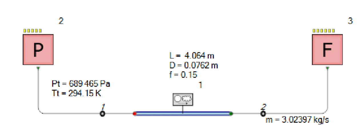
Pressure drop assessment

Table 1 Pressure drop Input data

Inputs Pt inlet Pa 689 465 Tt K 294.15 ṁ kg/s 3.02395 𝒇̅ - 0.15 L m 4.064 D m 0.0762

Table 2 Pressure drop Output Values

Inlet Outlet FM Hand calculation Deviation FM Hand calculation Deviation Mach 0.244756 0.244761 0.00% 0.516405 0.516482 0.01% Ts K 290.67 290.67 0.00% 279.248 279.247 0.00% Pt Pa 368456 368430 0.01% P Pa 661 314 661 315 0.00% 307 154 307 132 -0.01%

(33)

From comparison between FM results and the hand calculations, FM gives accurate results in agreement with theory.

2.3.2 Heat transfer model

Figure 8 Heat-exchanger component

The type of heat exchanger used in the ECS model is the Flowmaster Thermal Heat-Exchanger. This component can be inserted in compressible simulations to model the heat exchange between two gas streams. The amount of heat transfer is defined by the effectiveness or the heat load (also called thermal duty), Q, and the pressure drop is calculated by specifying a constant pressure drop coefficient for each stream.

Thermal simulation with dry air

The maximum possible heat transfer rate in a heat exchanger (HX) is calculated assuming an ideal heat exchanger of infinite area where one of the outlet streams (cold or hot) reaches the inlet temperature of the opposite stream, i.e. the maximum temperature difference |𝑇_0,1,𝐻− 𝑇_0,1,𝐶| is

(34)

reached. It can be shown that the stream undergoing the maximum temperature difference has also the minimum ṁ·Cp value. [23] Assuming constant heat capacities, the maximum heat transfer can

be written as

𝑸̇𝒎𝒂𝒙= (𝒎̇𝑪𝒑)_𝒎𝒊𝒏(𝑻𝟎,𝟏,𝑯− 𝑻𝟎,𝟏,𝑪) (13)

To calculate the minimum value of ṁ·Cp, values for the hot and cold streams must be compared.

(𝒎̇ ∙ 𝑪𝒑)_𝒎𝒊𝒏 = 𝑴𝒊𝒏 {(𝒎̇ ∙ 𝑪𝒑)_𝑯, (𝒎̇ ∙ 𝑪𝒑)_𝑪} (14)

Integrating the First law (Equation 9) with respect to total temperature and assuming constant heat capacity, it follows that the energy expression for the cold and hot streams are

𝑸𝑯= (𝒎̇𝑪𝒑)_𝑯(𝑻𝟎,𝟐− 𝑻𝟎,𝟏)_𝑯 (15)

𝑸𝑪= (𝒎̇𝑪𝒑)_𝑪(𝑻𝟎,𝟐− 𝑻𝟎,𝟏)_𝑪 (16)

The heat exchanger’s thermal effectiveness, ε, is defined as the ratio of the actual heat transfer rate over the maximum possible heat transfer rate.

𝜺 =_𝑸̇|𝑸̇|

𝒎𝒂𝒙 (17)

The effectiveness can be related to two parameters referred to as the Number of Transfer Units (NTU) and the ratio of Capacity coefficients (Cr).

𝑁𝑇𝑈 = 𝑈𝐴 (𝑚̇𝐶_𝑝) 𝑚𝑖𝑛 𝐶𝑟 = (𝑚̇𝐶𝑝)_𝑚𝑖𝑛 (𝑚̇𝐶_𝑝) 𝑚𝑎𝑥

Thus, it is possible to characterize the thermal performance of a heat exchanger with the functional relation

𝜀 = 𝑓(𝑁𝑇𝑈, 𝐶_𝑟)

Thermal performance can also be presented in terms of the ratio 𝑄/(𝐼𝑇𝐷 ∙ 𝐴), where ITD stands for Inlet Temperature Difference, (𝑇0,1,𝐻− 𝑇0,1,𝐶), and A is the exchange area.

(35)

From now, the parameter 𝑄/(𝐼𝑇𝐷 ∙ 𝐴) will be referred to as the performance capability. Its derivation is a direct consequence of the ε-NTU method. [24] As a matter of fact, the performance capability is simply 𝜀 ∙(𝑚̇𝐶𝑝)𝑚𝑖𝑛

𝐴 and the functional relationship is that of the effectiveness

multiplied by 𝜀 ∙(𝑚̇𝐶𝑝)𝑚𝑖𝑛

𝐴 .

𝑄/(𝐼𝑇𝐷 ∙ 𝐴) = 𝑓(𝑁𝑇𝑈, 𝐶_𝑟) ∙(𝑚̇𝐶𝑝)𝑚𝑖𝑛

𝐴 .

Humid air mixture

The presence of humidity in the air has a great impact on heat-exchangers performance, essentially when condensation or evaporation occurs.

The water content in the air can be specified by the humidity ratio, the relative humidity or the specific humidity. The humidity ratio, w, is defined as the ratio of the amount of water vapor (mass) by the amount of dry air. The fact that the humidity ratio is defined with respect to dry air and not the total gas mixture (dry air and water vapor) is advantageous because dry air component of the mixture is generally conserved, while water vapor can easily change between process units. Humidity ratio: 𝑤 = 𝑚𝑣

𝑚𝑎

The relative humidity is defined by considering the maximum amount of water vapor that dry air can dissolve at a given temperature and pressure.

Relative humidity: 𝜙 = 𝑃

𝑃0_(𝑇)

P is the partial pressure of water vapor in the gas mixture and 𝑃0_{(𝑇) is the saturation vapor pressure}

of water at the temperature of the gas mixture.

Finally, the specific humidity is defined with respect to the total amount (mass) of gas mixture. Specific humidity: 𝑥 = 𝑚𝑣

(36)

Thermal simulation with humid air

To develop the thermal equation using humid air, we first need to choose reference values for energies for water and air. The most common choice is to assign zero enthalpy for liquid water at 0°C, and zero enthalpy for dry air at 0°C. Then, the enthalpy of the gas mixture per unit mass of dry air can be defined as, [25]

𝒉 ≡ 𝑯̇

𝒎̇𝒂= 𝑪𝒑𝒂𝒊𝒓(𝑻 − 𝑻𝒓𝒆𝒇) + 𝒘 [𝒉𝒍𝒂𝒕𝒆𝒏𝒕+ 𝑪𝒑𝒗𝒂𝒑𝒐𝒓(𝑻 − 𝑻𝒓𝒆𝒇)] (18)

Applying mass and energy balance between the heat exchanger, the following relations are obtained:

 mass balance on dry air: 𝑚̇𝑎,1 = 𝑚̇𝑎,2

 mass balance for water: 𝑚̇𝑎,1𝑤 = 𝑚̇𝑎,2𝑤

 Energy balance = 𝑚̇_𝑎,1ℎ₁+ 𝑄̇ = 𝑚̇_𝑎,1ℎ₂

Thus, when Q and T1 are known and no condensation or evaporation occurs, the following equation

must be solved to find the outlet temperature T2

𝑸̇ = 𝒎̇𝒂,𝟏(𝑪𝒑𝒂𝒊𝒓(𝑻𝟐− 𝑻𝟏) + 𝒘 [𝑪𝒑𝒗𝒂𝒑𝒐𝒓(𝑻𝟐− 𝑻𝟏)]) (19)

When there is liquid water at the inlet or outlet, the problem becomes more complex as evaporation or condensation can occur. An additional term must be added to Equation 18 to take into account the liquid water content.

Flow pressure simulation

The same governing equations for pipes (Equations 1 to 9) can be used to model heat exchangers’ pressure loss. The heat duty must be taken into account by using Equation 15 or Equation 16. The assumption of no change in potential energy, constant compressibility factor and constant heat capacity ratio remains.

After algebraic manipulation of Equations 1, 2, 4, and 5, we can finally write the following differential equation.[26]

(37)

𝑑𝑀2 𝑀2 = 𝐹𝑇0 𝑑𝑇_𝑜 𝑇_𝑜 + 𝐹𝑓 𝑓𝑑𝑥 𝐷 Where 𝐹_𝑇0 = (1+𝛾𝑀 2₎₍₁₊𝛾−1 2 𝑀 2₎ 1−𝑀2 and 𝐹𝑓 = 𝛾𝑀2(1+𝛾−1 2 𝑀 2₎ 1−𝑀2 . After integration, 𝒍𝒏 (𝑴𝟐𝟐 𝑴_𝟏𝟐) = 𝑭̅𝑻𝟎𝒍𝒏 ( 𝑻𝟎,𝟐 𝑻𝟎,𝟏) + 𝑭 ̅_𝒇𝒇̅𝑳 𝑫 (20)

Where 𝐹̅𝑇0 and 𝐹̅𝑓 are the average values of 𝐹𝑇0 and 𝐹𝑓 between M1 and M2, respectively. Besides,

unlike the pipe component, the friction factor is not calculated by FM as a function of the Reynolds number in heat exchangers. In fact, the pressure drop coefficient, 𝑓̅𝐿

𝐷, is simply assumed as a

constant average value throughout the entire stream and must be entered in FM by the user. At last, the total temperature at the outlet T0,2 can be calculated independently using Equation 15 or

Equation 16.

Heater-cooler component

The Heater-cooler component allows heating or cooling of a fluid in a straightforward manner when the exact heating flow is known. The heat flow (positive or negative) is entered and FM computes the outlet temperature according to Equation 15 if heat is removed from the fluid (Equation 16 if heat is added).

(38)

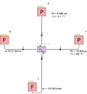
Heat-exchanger assessment

Table 3 Heat-Exchanger Input data Cold Stream Hot Stream

Tt inlet K 328.75 497.65 Pt inlet Pa 82 937 272 335 ṁ kg/s 1.796075 0.441421 𝐟̅𝐋/𝐃 - 4.435 55.455 A m2 0.0645161 0.0135484 Q W 66220

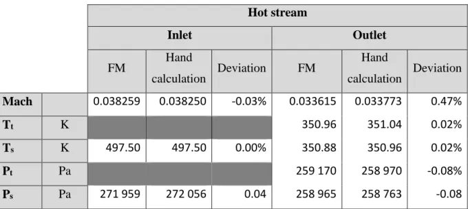
Table 4 Hot stream outputs Hot stream Inlet Outlet FM Hand calculation Deviation FM Hand calculation Deviation Mach 0.038259 0.038250 -0.03% 0.033615 0.033773 0.47% Tt K 350.96 351.04 0.02% Ts K 497.50 497.50 0.00% 350.88 350.96 0.02% Pt Pa 259 170 258 970 -0.08% Ps Pa 271 959 272 056 0.04 258 965 258 763 -0.08

(39)

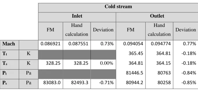
Table 5 Cold stream outputs Cold stream Inlet Outlet FM Hand calculation Deviation FM Hand calculation Deviation Mach 0.086921 0.087551 0.73% 0.094054 0.094774 0.77% Tt K 365.45 364.81 -0.18% Ts K 328.25 328.25 0.00% 364.81 364.15 -0.18% Pt Pa 81446.5 80763 -0.84% Ps Pa 83083.0 82493.3 -0.71% 80944.2 80258 -0.85%

It can be seen that most of the FM results obtained are consistent with the expected results by hand calculation. Therefore, temperature predictions for this component are reliable but tends to be less accurate as the temperature difference is greater than 100 K.

2.3.3 Fan model

Dimensional analysis

Fans are typically modeled by means of their performance maps made by their manufacturers. However, these maps are generally built for a given set of operating conditions: constant fan diameter or constant rotational speed for instance. Therefore, dimensional analysis is necessary to adjust the performance maps to different operating conditions.

The performance of a family of geometrically similar fans, under the assumptions of low-speed (Mach<0.3) and same representative roughness surface finish length, can be expressed as a function of: [27]

 Flow rate 𝑄̇ [m3_/s]

 Rotor speed N [RPM]  Fluid density 𝜌 [kg/m3_]

(40)

 Fluid viscosity 𝜇 [kg/m·s]  Rotor diameter 𝐷 [m]  Power developed 𝑊̇ [J/s]  Pressure 𝑝 [Pa]

 Efficiency 𝜂

By performing dimensional analysis (Buckingham’s π-theorem), four dimensionless groups are obtained: [28]  𝜋₁ = 𝑄̇ 𝑁𝐷3 𝐹𝑙𝑜𝑤 𝑐𝑜𝑒𝑓𝑓𝑖𝑐𝑖𝑒𝑛𝑡  𝜋₂ = 𝑃 𝜌𝑁2_𝐷2 𝑃𝑟𝑒𝑠𝑠𝑢𝑟𝑒 𝑐𝑜𝑒𝑓𝑓𝑖𝑐𝑖𝑒𝑛𝑡  𝜋3 = 𝑊 𝜌𝑁3_𝐷5 𝑃𝑜𝑤𝑒𝑟 𝑐𝑜𝑒𝑓𝑓𝑖𝑐𝑖𝑒𝑛𝑡  𝜋₄ = 𝜌𝑁𝐷2 𝜇 𝐹𝑎𝑛 𝑅𝑒𝑦𝑛𝑜𝑙𝑑𝑠 𝑛𝑢𝑚𝑏𝑒𝑟

Therefore, if the operating conditions of two geometrically similar fans are dynamically similar, then all the dimensionless groups are the same. Moreover, since the efficiency 𝜂 does not appear in the dimensionless groups, we must then conclude that two dynamically similar flows have the same efficiency.

We can reduce the number of dimensionless groups by eliminating 𝜋₃ since the Power coefficient can be written as being equal to:

𝑊 𝜌𝑁3_𝐷5 = 1 𝜂× 𝑄̇ 𝑁𝐷3× 𝑃 𝜌𝑁2_𝐷2

Furthermore, in most cases, the Reynolds number is assumed constant (turbulent regime) and only 𝜋₁, 𝜋₂ are considered. As shown on Figure 10, this simplification holds true for a wide range of Flow coefficient values but deviates to some extent at low speeds because of unsteady Reynolds number (laminar regime). At very high speeds, the unsteadiness is due to cavitation.

The efficiency, defined as the ratio between the shaft power transferred to the fluid and the power to drive the fan, can be introduced with respect to the flow, pressure and power coefficients.

(41)

𝜂 =𝑄̇𝑃

𝑊 =

𝜋₁∙ 𝜋₂ 𝜋₃ As far as dimensional analysis can be taken, 𝑄

𝑁𝐷3,

𝑃

𝜌𝑁2_𝐷2 and 𝜂 are the dimensionless groups to be considered. However, the actual relationship between them must be ascertained experimentally.

𝜂 = 𝑓 ( 𝑄̇ 𝑁𝐷3) 𝑃 𝜌𝑁2_𝐷2 = 𝑓 ( 𝑄̇ 𝑁𝐷3)

Finally, the well-known Fan laws, which are simply the ratio of the same dimensionless group for two different operating conditions are

𝑄̇₁ = 𝑄̇₂(𝑁1 𝑁₂) ( 𝐷1 𝐷₂) 3 𝑝₁ = 𝑝₂(𝜌1 𝜌₂) ( 𝑁₁ 𝑁₂) 2 (𝐷1 𝐷₂) 2

(42)

Fan model within Flowmaster

Figure 11 Fan component

Fans in FM are modeled using the fan component shown in Figure 11. In order to function properly, the user must supply two performance maps: static pressure increase vs. flow rate and polytropic efficiency vs. flow rate. Clearly, the maps are only accurate for a specific speed and fan diameter. For other sizes and speeds, the efficiency and pressure rise are approximated using the fan laws. The operating conditions for which the maps were built must be specified in the Design Point Data feature in FM.

FM uses a slightly different version of the fan laws adding a correction factor:

𝑸̇𝒓𝒆𝒇= 𝐐̇ ( 𝑵𝒓𝒆𝒇 𝑵 ) ( 𝑫𝒓𝒆𝒇 𝑫 ) 𝟑 𝒁 (21) ∆𝑷𝒔,𝒓𝒆𝒇 = ∆𝑷𝒔( 𝝆_𝒓𝒆𝒇 𝝆 ) ( 𝑵_𝒓𝒆𝒇 𝑵 ) 𝟐 (𝑫_𝑫𝒓𝒆𝒇)𝟐𝒁 (22)

The correction factor is defined as [30]

𝒁 = 𝟏 𝟏+(𝑴−𝟏)(𝟏−𝜼𝑨) (23) Where 𝐴 = 𝛾 (𝛾−1) ((𝑃0,2 𝑃0,1) (𝛾−1) 𝛾𝜂 −1) (𝑃0,2 𝑃0,1−1) and 𝑀 = ( 𝑁 𝑁𝑟𝑒𝑓) 2 ( 𝐷 𝐷𝑟𝑒𝑓) 2 ( 𝑇𝑠 𝑇𝑠,𝑟𝑒𝑓).

Additionally, the total temperature rise is computed using the definition of the polytropic efficiency.

(43)

𝑻_𝟎,𝟐 𝑻𝟎,𝟏= ( 𝑷_𝟎,𝟐 𝑷𝟎,𝟏) (𝜸−𝟏) 𝜸𝜼𝒑 (24)

Fan choking and surging are not modeled within this component. However, the choking flow rate at the design conditions can be specified as an upper limit for the performance maps. FM will then use the pressure and efficiency at this point for any flow rate above this limit. The same considerations apply to fan surging. The surging flow rate can be specified as a lower limit and FM will use the pressure increase and efficiency at this point for any flow rate below this limit.

Fan performance maps

The performance maps taken from FM and used for the assessment are showed below. These maps correspond to the reference conditions presented in Table 6, where the flow rate is measured at the fan inlet.

(44)

Figure 13 Fan pressure increase plot

If the fan is operated at a different speed or with a different fan diameter than those at the reference, the actual flow rate cannot be used directly to find the efficiency and pressure increase on the maps. The equivalent flow must first be calculated. With the equivalent flow, efficiency and pressure increase can be read from the maps.

Fan assessment

Table 6 Fan Reference data

Ts inlet K 380.55

ρ kg/m3 0.39038

Fan diameter m 0.118

N RPM 44962

Choking rate m3_/s _1.02

(45)

Table 7 Fan Inlet conditions Tt inlet K 343.35 Pt inlet Pa 74048.5 ṁ kg/s 0.6188 N RPM 41982 Fan diameter m 0.118 Pipe diameter m 0.11938

Since the operating speed is different from the reference, the reference flow rate and the actual pressure increase are calculated and showed in Table 8 among other intermediate results.

Table 8 Fan Efficiency and actual pressure increase

Qactual m3/s 0.8405

Qref m3/s 0.9038

η (from map) % 79.145

ΔPs, ref (from map) Pa 2691.5

M 0.780

A (pipe cross area) 1.240

Z 1.004

ΔPs, actual Pa 4443.0

Table 9 Fan Output values

Inlet Outlet FM Hand calculation Deviation (%) FM Hand calculation Deviation (%) Mach 0.20298 0.20299 0.00 0.19331 0.19325 -0.03 Tt K 350.46 350.52 0.02

(46)

Ts K 340.54 340.54 0.00 347.86 347.92 0.02

Pt Pa 78 376.4 78 410.3 0.04

Ps Pa 71 951.8 71 951.6 0.00 76 360.8 76 394.8 0.04

The deviation in outlet pressure is relatively small. Nevertheless, the difference is mainly due to the precision when reading the maps (η and ΔPs,ref).

2.3.4 Compressor model

Figure 14 Compressor component

Compressor dimensional analysis

Compressors are used to increase the pressure of a gas. Like fans, compressor modeling requires information on their performance provided by the manufacturer. To derive the performance relations, dimensional analysis of compressors is accomplished. Indeed, compressibility effects must be taken into account by considering additional parameters. In this analysis, the stagnation speed of sound, 𝑎₀, at the entry of the compressor and the ratio of specific heats, 𝛾, are chosen for this task. In fact, the Mach number can take values up to one whereas with fans, we assumed Mach<03. Also, instead of considering the pressure as a performance parameter, the isentropic stagnation enthalpy change ∆ℎ0,𝑖𝑠𝑒 is selected. Instead of the volume flow rate 𝑄̇ and density 𝜌, the

(47)

mass flow rate 𝑚̇ and total density 𝜌₀ are employed. By convenience, ∆ℎ_{0,𝑖𝑠𝑒}, 𝜂_𝑖𝑠𝑒 and 𝑊 are considered as the dependent variables while the remaining variables 𝜇, 𝑁, 𝐷, 𝑚̇, 𝜌_0,1, 𝑎_0,1 and 𝛾 are the independent variables. Therefore, in light of what has been previously said, the compressor performance can be expressed functionally as

∆ℎ_{0,𝑖𝑠𝑒}, 𝜂_𝑖𝑠𝑒, 𝑊̇ = 𝑓(𝜇, 𝑁, 𝐷, 𝑚̇, 𝜌_0,1, 𝑎_0,1, 𝛾) From dimensional analysis, seven dimensionless groups are obtained:[29]

∆ℎ_{0,𝑖𝑠𝑒} 𝑎_0,12 , 𝜂𝑐, 𝑊̇ 𝜌_0,1𝑎_0,13 𝐷2 = 𝑓 ( 𝑚̇ 𝜌_0,1𝑎_0,1𝐷2, 𝜌_0,1𝑎_0,1𝐷 𝜇 , 𝑁𝐷 𝑎_0,1, 𝛾)

In practice, it is not very convenient to use these groups. In reality, the majority of turbo-compressors manufacturers will deal with a different set of dimensionless groups that will be derived herein by straightforward transformations.

For an isentropic process and assuming constant specific heat, the equation below is always verified. [31] 𝑻𝟎,𝟐𝒊𝒔𝒆 𝑻𝟎,𝟏 = ( 𝑷𝟎,𝟐 𝑷𝟎,𝟏) (𝜸−𝟏) 𝜸⁄ (25) The isentropic specific stagnation enthalpy change, ∆ℎ_{0,𝑖𝑠𝑒}= 𝐶_𝑝(𝑇_{0,2𝑖𝑠𝑒}− 𝑇_0,1), is then

∆ℎ_{0,𝑖𝑠𝑒} = 𝑇_0,1((𝑃0,2 𝑃_0,1)

(𝛾−1) 𝛾⁄

− 1)

Also, 𝐶𝑝 = 𝛾𝑅 (𝛾 − 1)⁄ and 𝑎0,12 = 𝛾𝑅𝑇0,1 = (𝛾 − 1)𝐶𝑝𝑇0,1. Hence,

∆ℎ0,𝑖𝑠𝑒 𝑎_0,12 = 1 𝛾 − 1(( 𝑃0,2 𝑃0,1 ) (𝛾−1) 𝛾⁄ − 1) →∆ℎ0,𝑖𝑠𝑒 𝑎_0,12 = 𝑓 (( 𝑃_0,2 𝑃0,1 ) , 𝛾)

The mass flow coefficient can be rewritten using the equation of state 𝜌0 = 𝑃0⁄𝑅𝑇0 and the

definition of stagnation speed of sound. 𝑚̇ 𝜌0,1𝑎0,1𝐷2 = 𝑚̇𝑅𝑇0,1 𝜌_0,1√𝛾𝑅𝑇0,1𝐷2 = 𝑚̇√𝛾𝑅𝑇0,1 𝐷2_𝑃 0,1𝛾

(48)

The power coefficient term can also be transformed. 𝑊̇ 𝜌_0,1𝑎_0,13 𝐷2 = 𝑚̇𝐶_𝑝Δ𝑇₀ (𝜌_0,1𝑎_0,1𝐷2_)𝑎 0,12 = (𝑚̇√𝛾𝑅𝑇0,1 𝐷2_𝑃 0,1𝛾 )𝐶𝑝Δ𝑇0 𝑎_0,12 = ( 𝑚̇√𝛾𝑅𝑇0,1 𝐷2_𝑃 0,1𝛾 ) 1 (𝛾 − 1) Δ𝑇0 𝑇_0,1 → 𝑊 𝜌0,1𝑎0,13 𝐷2 = 𝑓 (𝑚̇√𝛾𝑅𝑇0,1 𝐷2_𝑃 0,1𝛾 ,Δ𝑇0 𝑇_0,1, 𝛾)

After considering the previous transformations, the new dimensionless groups can be functionally

expressed as 𝑃0,2 𝑃0,1 , 𝜂_𝑖𝑠𝑒,Δ𝑇0 𝑇0,1 = 𝑓 (𝑚̇√𝛾𝑅𝑇0,1 𝐷2_𝑃 0,1𝛾 ,𝜌0,1√𝛾𝑅𝑇0,1𝐷 𝜇 , 𝑁𝐷 √𝛾𝑅𝑇0,1 , 𝛾)

Further simplification can be accomplished for a compressor of constant diameter handling a single fluid by dropping R, 𝛾 and D. Consequently, the resulting variables can only be applied to map a unique compressor of a given size and compressing a specific gas. In addition, the term 𝜌0,1√𝛾𝑅𝑇0,1𝐷

𝜇 ,

which is a form of the Reynolds number, can also be dropped assuming turbulent regime. Under these conditions, the previous relation turns out to be

𝑃_0,2 𝑃0,1 , 𝜂𝑖𝑠𝑒, Δ𝑇₀ 𝑇0,1 = 𝑓 (𝑚̇√𝑇0,1 𝑃0,1 , 𝑁 √𝑇0,1 , )

The performance variable Δ𝑇0

𝑇0,1 can also be dropped because it can be back calculated if the efficiency and the pressure ratio are known. In fact,

𝜂_𝑖𝑠𝑒≡ 𝑚𝑖𝑛𝑖𝑚𝑢𝑚 𝑒𝑛𝑒𝑟𝑔𝑦 𝑑𝑖𝑓𝑓𝑒𝑟𝑒𝑛𝑐𝑒 𝑝𝑜𝑠𝑠𝑖𝑏𝑙𝑒 𝑓𝑜𝑟 𝑡ℎ𝑒 𝑓𝑙𝑢𝑖𝑑 𝑎𝑐𝑡𝑢𝑎𝑙 𝑤𝑜𝑟𝑘 𝑖𝑛𝑝𝑢𝑡 𝑡𝑜 𝑡ℎ𝑒 𝑓𝑙𝑢𝑖𝑑 [31] 𝜼_𝒊𝒔𝒆 =𝒎̇𝑪𝒑(𝑻𝟎,𝟐𝒊𝒔𝒆−𝑻𝟎,𝟏) 𝒎̇𝑪𝒑(𝑻𝟎,𝟐−𝑻𝟎,𝟏) (26) But 𝑇_{0,2𝑖𝑠𝑒} is equal to 𝑇_𝑡,1(𝑃0,2 𝑃0,1) (𝛾−1) 𝛾⁄ from Equation 25. → 𝜂_𝑖𝑠𝑒= ((𝑃_𝑃0,2 0,1) (𝛾−1) 𝛾⁄ − 1) Δ𝑇₀/𝑇_0,1

(49)

Furthermore, it is common practice to express the mass flow rate and speed variables in terms of their corrected form.

𝑪𝒐𝒓𝒓𝒆𝒄𝒕𝒆𝒅 𝒎𝒂𝒔𝒔 𝒇𝒍𝒐𝒘 𝒓𝒂𝒕𝒆: 𝒎̇√𝑻𝟎,𝟏 𝑻𝒓𝒆𝒇 ⁄ 𝑷𝟎,𝟏⁄𝑷𝒓𝒆𝒇 (27 ) 𝑪𝒐𝒓𝒓𝒆𝒄𝒕𝒆𝒅 𝒔𝒑𝒆𝒆𝒅: 𝑵 √𝑻𝟎,𝟏⁄𝑻𝒓𝒆𝒇 (28 )

The corrected mass flow rate (CMFR) and the corrected speed represent the mass flow and rotational speed that would be measured if the compressor was operating at an arbitrary reference pressure and temperature; standard sea-level conditions for instance.

To conclude, we can finally express the performance relation as

𝑷𝟎,𝟐 𝑷𝟎,𝟏= 𝒇 ( 𝒎̇√𝑻𝟎,𝟏⁄𝑻𝒓𝒆𝒇 𝑷𝟎,𝟏⁄𝑷𝒓𝒆𝒇 , 𝑵 √𝑻𝟎,𝟏⁄𝑻𝒓𝒆𝒇 ) (29) 𝜼_𝒊𝒔𝒆 = 𝒇 (𝒎̇√𝑻𝟎,𝟏 𝑻𝒓𝒆𝒇 ⁄ 𝑷𝟎,𝟏⁄𝑷𝒓𝒆𝒇 , 𝑷𝟎,𝟐 𝑷𝟎,𝟏 ) (30)

Notice that the new variables on the right-hand side are no longer dimensionless.

Humid air effects

Presence of water vapor changes the air properties such as Cp, γ, and R. Of course, the deviation

from the dry air state increases as more vapor is present. Yet, the compressor dimensional analysis done previously applies only to perfect gases with constant caloric properties. According to [32], ignoring this deviation can lead to 2-3% efficiency errors. However, under 10% specific humidity, humid gas mixture can be considered as dry [33].

Samuel’s and Gales’s correction factors [34] can be useful to take into account the effects of humidity on R and 𝛾. By doing so, the new corrected mass flow rate and corrected rotational speed numbers become

 𝑚̇√𝑇0,1⁄𝑇𝑟𝑒𝑓

𝑃0,1⁄𝑃𝑟𝑒𝑓 √

𝑅𝑚𝑖𝑥

(50)

 𝑁 √𝑇0,1⁄𝑇𝑟𝑒𝑓

1 √𝑅𝑚𝑖𝑥∙𝛾𝑚𝑖𝑥

Flowmaster’s compressor model

FM’s definition of compressor pressure ratio is slightly different than what was presented above. FM uses the outlet static pressure instead of the outlet total pressure.

𝑃𝑟𝑒𝑠𝑠𝑢𝑟𝑒 𝑟𝑎𝑡𝑖𝑜 =𝑂𝑢𝑡𝑙𝑒𝑡 𝑠𝑡𝑎𝑡𝑖𝑐 𝑝𝑟𝑒𝑠𝑠𝑢𝑟𝑒 𝐼𝑛𝑙𝑒𝑡 𝑡𝑜𝑡𝑎𝑙 𝑝𝑟𝑒𝑠𝑠𝑢𝑟𝑒 =

𝑃_𝑠,2 𝑃_0,1

Two 3D performance maps represented by the functions below must be supplied prior to running a simulation in order to fully characterize the compressor.

𝑷𝒔,𝟐 𝑷𝟎,𝟏= 𝒇 ( 𝒎̇√𝑻𝟎,𝟏⁄𝑻𝒓𝒆𝒇 𝑷𝟎,𝟏⁄𝑷𝒓𝒆𝒇 , 𝑵 √𝑻𝟎,𝟏⁄𝑻𝒓𝒆𝒇 ) (31) 𝜼_𝒊𝒔𝒆 = 𝒇 (𝒎̇√𝑻𝟎,𝟏 𝑻𝒓𝒆𝒇 ⁄ 𝑷𝟎,𝟏⁄𝑷𝒓𝒆𝒇 , 𝑷𝒔,𝟐 𝑷𝟎,𝟏) (32)

Humidity correction is not supported by FM, so R and γ were assumed constant and equal to dry air values in our ECS model.

Compressor performance maps

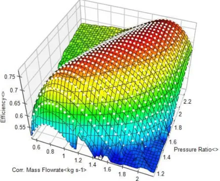
Figure 15 shows a typical compressor performance map from Garret’s [35]. The contour lines represent constant efficiencies whereas the perpendicular lines represent constant corrected speeds. From a map like this, it is possible to extract all the necessary information needed to predict compressor’s outlet conditions of temperature, pressure and power consumption.

From the same figure, one can also estimate the surge and choke lines. These are two important lines that show the operating limits of the equipment. The surge limit is the left hand boundary green line. This region is characterized by flow instability where the mass flow is too small for the generated boost and spinning. Operating at this limit may cause reversal of airflow through the unit. On the other hand, the choke line in red is characterized by a low backpressure and high

(51)

compressor output at a given speed. The gas velocity and gas flow rate cannot go beyond the value at the choke point.

Finally, the dashed line represents the operating line. Its exact position is not a property of the compressor, but rather of the rest of the system. [36] For the ECS pack, the operating line is contingent upon many factors such as the flow area downstream of the compressor, the turbine’s throat area and the amount of heat removed by the heat-exchangers. Nevertheless, the system designer will try to locate the compressor’s operating line so as to allow for operating in the higher efficiency range.

Figure 15 Typical compressor performance map [35]

Figures 16 and 17 are examples of performance maps used in FM simulation. Though, surge and choke flow rates are specified elsewhere in the component’s option screen. They can be specified as constants values or as functions of rotational speed.

(52)

Figure 16 Compressor pressure ratio surface

(53)

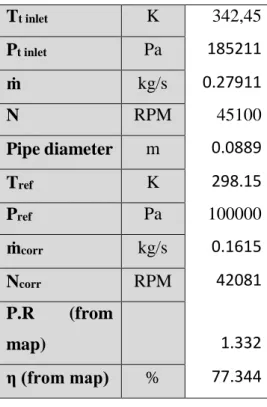
Compressor assessment

Table 10 Compressor Input values

Tt inlet K 342,45 Pt inlet Pa 185211 ṁ kg/s 0.27911 N RPM 45100 Pipe diameter m 0.0889 Tref K 298.15 Pref Pa 100000 ṁcorr kg/s 0.1615 Ncorr RPM 42081 P.R (from map) 1.332 η (from map) % 77.344

Table 11 Compressor Output values

Inlet Outlet FM Hand calculation Deviation (%) FM Hand calculation Deviation (%) Mach 0.06448 0.06449 0.01 0.05087 0.05088 0.01 Tt K 380.54 380.54 0.00 Ts K 342.17 342.17 0.00 380.35 380.35 0.02 Pt Pa 247128 247243 0.05 Ps Pa 184 673 184 673 0.00 246796 246796 0.04

(54)

2.3.5 Turbine model

Figure 18 Turbine component

Turbines transform fluid pressure into useful work by the action of the moving fluid on the blades so that they move and impart rotational energy to the rotor assembly. The dimensional analysis of the expansion process in turbines is similar to the compression process. This means that the performance is determined by the same dimensionless groups.

𝑃_0,2 𝑃0,1 , 𝜂𝑖𝑠𝑒, Δ𝑇₀ 𝑇0,1 = 𝑓 (𝑚̇√𝑇0,1⁄𝑇𝑟𝑒𝑓 𝑃0,1⁄𝑃𝑟𝑒𝑓 , 𝑁 √𝑇0,1⁄𝑇𝑟𝑒𝑓 , )

However, since expansion involves decreasing the pressure of the entering fluid and extracting energy, the isentropic efficiency is defined differently.

𝜂_𝑖𝑠𝑒 ≡ 𝐴𝑐𝑡𝑢𝑎𝑙 𝑤𝑜𝑟𝑘 𝑑𝑜𝑛𝑒 𝑏𝑦 𝑡ℎ𝑒 𝑓𝑙𝑢𝑖𝑑 𝑀𝑎𝑥𝑖𝑚𝑢𝑚 𝑒𝑛𝑒𝑟𝑔𝑦 𝑑𝑖𝑓𝑓𝑒𝑟𝑒𝑛𝑐𝑒 𝑝𝑜𝑠𝑠𝑖𝑏𝑙𝑒 𝑓𝑜𝑟 𝑡ℎ𝑒 𝑓𝑙𝑢𝑖𝑑 ≈ 𝑚̇𝐶_𝑝(𝑇_0,1− 𝑇_0,2) 𝑚̇𝐶_𝑝(𝑇_0,1− 𝑇_{0,2𝑖𝑠𝑒}) 𝜼𝒊𝒔𝒆= (𝑻𝟎,𝟏−𝑻𝟎,𝟐)/𝑻𝟎,𝟏 (𝟏−(𝑷𝟎,𝟐 𝑷𝟎,𝟏) (𝜸−𝟏) 𝜸⁄ ) (33)

(55)

Flowmaster’s turbine model

In FM, the turbine pressure ratio is defined in terms of total pressure.

𝑃𝑟𝑒𝑠𝑠𝑢𝑟𝑒 𝑟𝑎𝑡𝑖𝑜 = 𝐼𝑛𝑙𝑒𝑡 𝑡𝑜𝑡𝑎𝑙 𝑝𝑟𝑒𝑠𝑠𝑢𝑟𝑒 𝑂𝑢𝑡𝑙𝑒𝑡 𝑡𝑜𝑡𝑎𝑙 𝑝𝑟𝑒𝑠𝑠𝑢𝑟𝑒=

𝑃_0,1 𝑃_0,2 As a result, the two required maps for turbine characterization are:[29]

𝑷𝟎,𝟏 𝑷_𝟎,𝟐 = 𝒇 ( 𝒎̇√𝑻𝟎,𝟏⁄𝑻𝒓𝒆𝒇 𝑷_𝟎,𝟏⁄𝑷_𝒓𝒆𝒇 , 𝑵 √𝑻𝟎,𝟏⁄𝑻𝒓𝒆𝒇 ) (34) 𝜼𝒊𝒔𝒆 = 𝒇 ( 𝒎̇√𝑻𝟎,𝟏⁄𝑻𝒓𝒆𝒇 𝑷𝟎,𝟏⁄𝑷𝒓𝒆𝒇 , 𝑷𝟎,𝟏 𝑷𝟎,𝟐) (35)

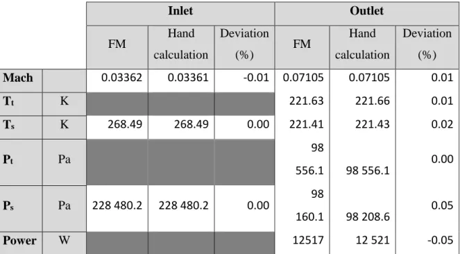
Differing from the compressor component, FM’s turbine component allows specifying a constant efficiency (not as a function of corrected mass flow rate and corrected rotational speed). This option makes the component to be more flexible to work with. For instance, when only data of PR vs. corrected mass flow rate is available for a constant efficiency, a simulation can still be solved. The corresponding rotational speed will be unknown, but sometimes one might be only interested in finding the outlet fluid conditions. For the assessment, only a PR vs. corrected mass flow rate map is supplied. The efficiency and corrected speed are chosen arbitrarily.

The power output from the turbine (actual work done by the fluid) is a very important information for simulation of the ACM as we will see later. To calculate the isentropic efficiency, we’ve approximated the power output by assuming a constant specific heat. In fact, this reasonable approximation has lead us to develop simple relations to predict outlet temperature. Now, to calculate the power output from the turbine we should write

𝐴𝑐𝑡𝑢𝑎𝑙 𝑤𝑜𝑟𝑘 𝑑𝑜𝑛𝑒 𝑏𝑦 𝑡ℎ𝑒 𝑓𝑙𝑢𝑖𝑑 = 𝑚̇ ∫ 𝐶_𝑝(𝑇)𝑑𝑇

𝑇𝑡,2

𝑇𝑡,1

However, FM approximates the power output by using the average specific heat.

𝑷𝒐𝒘𝒆𝒓 𝒐𝒖𝒕𝒑𝒖𝒕 = 𝒎̇ ∙ 𝑪𝒑 𝒂𝒗𝒈∙ ∆𝑻𝟎 = 𝒎̇ (

𝑪_𝒑( 𝑻𝟎,𝟏)+𝑪𝒑( 𝑻𝟎,𝟐)

(56)

Turbine performance maps

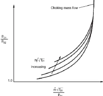
Turbines perform quite differently than compressors. In fact, it can be shown that the rotational speed has little effect on pressure ratio. Moreover, turbines are designed to work with high-pressure ratios ultimately leading to choked flow. These considerations are well reflected on their performance maps as in Figure 19. Figure 20 illustrates the performance map used for the assessment.

Figure 19 Typical Turbine map