Knowledge models for the engineering and optimization of photobioreactors

HAL Id: hal-02539915

https://hal.archives-ouvertes.fr/hal-02539915

Submitted on 10 Apr 2020

HAL is a multi-disciplinary open access

archive for the deposit and dissemination of

sci-entific research documents, whether they are

pub-lished or not. The documents may come from

teaching and research institutions in France or

abroad, or from public or private research centers.

L’archive ouverte pluridisciplinaire HAL, est

destinée au dépôt et à la diffusion de documents

scientifiques de niveau recherche, publiés ou non,

émanant des établissements d’enseignement et de

recherche français ou étrangers, des laboratoires

publics ou privés.

of photobioreactors

Jeremy Pruvost, Jean-François Cornet

To cite this version:

Jeremy Pruvost, Jean-François Cornet. Knowledge models for the engineering and optimization of

photobioreactors. C.Posten; C.Walter. Microalgal Biotechnology: Potential and Production, De

Gruyter, pp.181-224, 2012, 9783110225020. �hal-02539915�

10 Knowledge models for the engineering and

optimization of photobioreactors

10.1 Introduction

The modeling of microalgal photosynthetic biomass production draws some sup-port from the abundant literature on bioprocess modeling, in particular when min-eral or CO2mass-transfer limitations on growth rates are considered in the same

way as substrate and O2-transfer limitations in engineered bacterial cultivation.

However, photosynthetic biomass growth exhibits highly specific features owing to its need for light energy: unlike dissolved nutrients, assumed to be homo-geneous in well-mixed conditions, light energy is heterohomo-geneously distributed in the culture due to absorption and scattering by cells, independently of the mixing conditions. As light is the principal energy source for photosynthesis, this heteroge-neity alone sets microalgal cultivation systems apart from other classical biopro-cesses, as they are generally limited by light transfer inside the culture media. Hence the design, optimization and control of photobioreactors (PBRs) require spe-cific approaches.

This chapter deals with developing useful knowledge models for engineering microalgal cultivation systems. Prerequisites and main concepts will be presented. Concrete illustrations will be given that use modeling to gain a deeper understand-ing of the complex influence of light transfer on the process, and to predict bio-mass productivities as a function of cultivation system engineering variables (espe-cially depth of culture) and operating settings (residence time and incident light flux) in both artificial constant light and natural sunlight conditions.

10.2 Theoretical background for radiation measurement and

handling

10.2.1 Main physical variables

Given the crucial importance of radiative transfer description in photobioreactor modeling, it is essential to have a broad overview of the main physical quantities and definitions involved in radiation measurement and theory, together with a thorough knowledge of the conversion factors linking the two main practical sys-tems of units (joules and micromoles of photons). There is often much confusion on these points in the microalgal growth modeling literature, conducive to misin-terpretation of related physical and physiological processes. This section gives a

brief summary of the definitions, units, roles and related sensors for the three main useful physical quantities in the field of PBR modeling.

Strictly speaking, these three quantities are all spectral quantities (their defini-tion holds for a small differential part of the electromagnetic spectrum d λ indi-cated by a subscript λ), but for simplicity, in what follows we will mainly consider mean averaged quantities for photosynthetically active radiation (PAR). Thus the absence of an λ subscript means that we are working with integral quantities such as

X = ∫

Δλ

Xλdλ, in which Δ λ corresponds to the range of wavelengths between 400

and 700 nm (PAR).

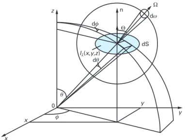
The first measurable variable (defined from an elemental oriented surface of reference d S) from which all the other useful and practical radiative quantities are deduced is the radiance, more generally named intensity I in many fields of physics (see Fig. 10.1). It is the ratio, in a given direction, of the solid angle d Ω and in a point of the oriented surface d S of the radiant power d E to the projected area on the perpendicular plane to the outward normal n:

I = dE dS cos Θ

[

]

This fundamental directional quantity may be integrated over the solid angle dω, giving the definition of the radiative flux density q such that the flux through an elemental surface dS of normal n is q ⋅ n dS.

In a given direction x, the projection of q is then:

qx = ∬ 4π I cos Θ dω = ∫ 0 2π ∫ 0 π

I cos Θ sin Θ d Θ d Φ

[

−1

.m−2

]

where cos Θ is the angle between the outward normal n and the considered direc-tion Ω (see Fig. 10.1), so defining the vectorial nature of this quantity.

In the field of PBR modeling, this flux density is mainly used to define the boundary conditions relative to given illumination conditions. In this case, only the incoming radiation on one hemisphere that penetrates the culture medium is of interest, giving the definition of the incident hemispherical radiant flux density or photon flux density (PFD) perpendicular to a reference surface:

q0= ∫ 0 2π ∫ 0 π/2 I0cos Θ sin Θ d Θ d Φ (10.3)

We note that the angular nature of this PFD may be different, and in some cases (especially for solar illumination) it may be useful to use a subscript to characterize this flux, such as q//for a collimated incidence, q⊥for the special case of normal

Fig. 10.1: Definition of the solid angle dω and of the associated intensity (strictly, radiance)

Iλ(x , y , z , Θ , Φ)from a fixed Cartesian r (x , y , z) or spherical r (r , θ , φ) frame of reference associated with a moving frame Ω (Θ , Φ) at a point P from which it is possible to derive all the radiative useful integral definitions for the description of radiative transfer in photobioreactor modeling.

density component can be measured with a flat cosine sensor, once a surface of reference has been chosen (Pottier et al. 2005).

The third and last integral quantity of interest, mainly to define the total radi-ant light energy available for photosynthesis and then formulate the kinetic and energy couplings, is the scalar spherical irradiance:

G = ∬ 4π I dω = ∫ 0 2π ∫ 0 π I sin Θ d Θ d Φ (W.m−2 or μmolhυ.s −1 .m−2) (10.4)

This quantity can be evaluated with a spherical quantum sensor, which strictly measures an energy fluence rate, assumed to be the irradiance if the sensor diame-ter is small compared with the characdiame-teristic extinction length for the radiation in the considered medium (Pottier et al. 2005).

We note that for modeling purposes, the angular pattern of the light must necessarily be known, to calculate the integrals of Equations (10.3) and (10.4) but is extremely difficult to measure. It can be postulated a priori or calculated from models of radiative emission. In all cases, this angular distribution ranges between two extremes:

– A collimated radiation giving the following relations between I0, q0and G0: q0= q//= ∫ 0 2π ∫ 0 π/2 I0 col

δ (Θ − Θcol) δ (Φ − Φcol) cos Θ sin Θ d Θ d Φ = I0 col

cos Θcol

= G0cos Θcol

– A diffuse isotropic radiation for which:

q0= q∩ = I0dif∫ 0 2π ∫ 0 π/2 cos Θ sin Θ d Θ d Φ = 2π1 2I0 dif _{= πI} 0dif = G0 2 10.2.2 Solar illumination

As previously defined, the light energy received by a solar cultivation system is represented by the hemispherical incident light flux density q, or photon flux den-sity (PFD), which has to be expressed within the range of photosynthetic active radiation (PAR), i.e. the 0.4–0.7 μm bandwidth. For example, the whole solar spec-trum at ground level covers the range 0.26–3 μm. The PAR range thus corresponds to almost 43 % of the full solar energy spectrum (for AM = 1.5 normalization).

As light is converted inside the culture volume, it is also necessary to add to the PFD determination a rigorous treatment of radiative transfer inside the culture (see later on in this chapter) strictly requiring knowledge of the angular distribu-tion of the incoming light, together with the light-source posidistribu-tioning with respect to the optical transparent surface of the cultivation system, i.e. the incident polar angle θ (Fig. 10.2). Ideally, collimated (direct) q_// and diffuse q∩ components of

radiation should be considered separately. By definition, the direction of a beam of radiation, which represents direct radiation received from the light source, will define the incident polar angle θ with the illuminated surface and the direct light flux density q//. By contrast, diffuse radiation cannot be defined by a single

inci-dent angle but has an angular distribution over the illuminated surface (on a 2 π solid angle for a plane). Because this angular distribution is unknown, an isotropic angular distribution (Lambertian behavior) is generally assumed when using the value of q∩.

10.3 Modeling light-limited photosynthetic growth in

photobioreactors

10.3.1 Overview of the modeling approach

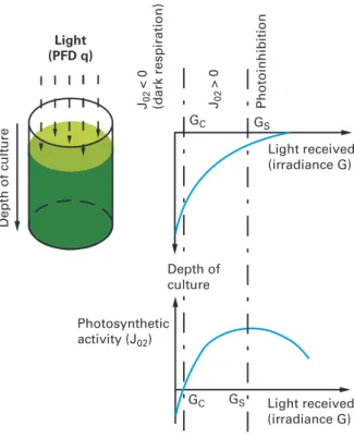
The photosynthetic activity (here represented by the specific oxygen production rate JO2) is directly related to the local light available inside the culture medium.

Fig. 10.2: Solar radiation on a microalgal cultivation system: incident angle and diffuse-direct

radiations (left), time course of solar sky path during the year (right).

characterized by progressive saturation of photosynthesis with irradiance G up to an irradiance of saturation Gs. For higher irradiances, photoinhibition processes

can occur with a negative influence on growth (Vonshak and Torzillo 2004). We also note that a threshold value of irradiance is needed to obtain positive growth. This value is termed the irradiance of compensation GC (corresponding to the

Fig. 10.3: Relation between light attenuation and photosynthetic growth in microalgal cultivation

systems.

“compensation point of photosynthesis”), which will prove relevant in the model-ing and understandmodel-ing of PBR operation (see later on in this chapter).

In cultivation systems, this nonlinear, complex response of photosynthesis has to be considered in combination with the light-attenuation conditions. In extreme cases of high light illumination and high light attenuation (high biomass concen-tration), cells in different physiological states will co-occur: some, close to the light source, may be photoinhibited, while others deep in the culture will receive no light. Ideally, the control of the system would require taking all these processes into account, a far from trivial task. As described next, modeling the kinetic coupling of photosynthetic growth with the radiation field inside cultivation systems will enable us to represent the impact of such effects on process efficiency. The main features of such a model are presented in the following sections.

10.3.2 Mass balances

The mass balance relates concentration in the cultivation system to kinetic rates of biological production (biomass, O2) or consumption (nutrients, CO2) and system

input and output. For a continuous system, assuming perfectly mixed conditions (continuous stirred tank reactor or CSTR model), the concentration C of a given element is then given by (Cornet et al. 2003; Pruvost et al. 2008; Pruvost 2011): dC

dt = 〈r (t)〉 + 1

τ(Ci− C) = 〈r (t)〉 + D (Ci− C) (10.5)

with <r> the mean volumetric production (biomass, metabolites) or consumption (nutrient) rate in the system, and τ the residence time resulting from the liquid flow rate of the feed of input concentration Ci(fresh medium) (with τ = 1 / D, where

D is the dilution rate).

Following the CSTR model, Equation (10.5) assumes homogeneous concentra-tion in the cultivaconcentra-tion system. Because of the slow growth rate of photosynthetic microorganisms compared with mixing time, this is usually the case, and so Equa-tion (10.5) holds. In some cases of large tubular cultivaEqua-tion systems without recy-cling, it may be necessary to work with the steady-state plug flow tubular reactor (PFTR) model, assuming a constant concentration only on a cross-section of the tube: ux dC dx − DL d2C dx2 = 〈r (x)〉 (10.6)

with uxthe linear velocity obtained along the flowing x-axis (ux= Q / S with Q the

liquid flow rate and S the tubular cross-section) and DLthe axial dispersion

coeffi-cient. This equation represents the evolution of concentration as a function of the distance x (length of the tube).

10.3.3 Stoichiometry of photosynthetic growth

10.3.3.1 Simple stoichiometric equations

Growth can be expressed in the form of a stoichiometric equation that can be deduced, for example, from a biomass elemental analysis (Roels 1983). As for bac-teria, the stoichiometric equation for photosynthetic growth in optimal conditions is found to be largely independent of the cultivated species, and depends only weakly on illumination and radiation field conditions (nutrient starvation can, by contrast, strongly influence biomass composition (Pruvost et al. 2011a)). Below are two examples for Chlamydomonas reinhardtii (Eq. (10.7)) and Arthrospira

platensis (Eq. (10.8)), emphasizing the difference in the photosynthetic quotient QP= υO2−CO2due to the nitrogen source (ammonium for C. reinhardtii vs. nitrate for

A. platensis), which is found to have the greatest impact on stoichiometric equation

CO2+ 0.593 H2O + 0.176 NH3+ 0.007 H2SO4 + 0.018 H3PO4% CH1.781O0.437N0.176S0.007P0.018+ 1.128 O2 (10.7) CO2+ 0.71 H2O + 0.14 HNO3+ 0.008 H2SO4 + 0.005 H3PO4% CH1.59O0.55N0.14S0.008P0.005+ 1.32 O2 (10.8)

As for any biological production, a stoichiometric equation is useful for converting biomass growth rates into substrate or product rates, for example to determine nutrient requirements (especially in terms of nitrogen, phosphorus and sulfur sour-ces for photosynthetic microorganisms). It is also practically useful for understand-ing the CO2/ O2exchange and mass-transfer limitations or the CO2-related pH time

course when the stoichiometric equation is expressed by the charge of ionic species (Cornet et al. 1998)

10.3.3.2 Structured stoichiometric equations

More sophisticated structured equations can be developed if a deep understanding of the coupling between energetics, kinetics and stoichiometry in the photosynthe-sis process at the cell level is sought (Roels 1983). These equations involve the stoichiometric cofactor balances such as NADPH,H+ _{in photosynthesis and the}

associated ATP production rate defining the P / 2e−_{ratio in the Z-scheme of}

photo-synthesis (Cornet et al. 1998). For example, in the case of A. platensis growth, the stoichiometric equation (Eq. (10.8)) may be rewritten, from a structured analysis of the P / 2e−_{ratio for each main cellular component (proteins, lipids, carbohydrates,}

etc.), and for a mean value of the incident PFD of 500 μmolhν.m–2.s–1as:

CO2+ 1.71 H2O + 0.14 HNO3+ 0.008 H2SO4+ 3.62 ATP + 2.62 (NADPH, H +

) #%JX

CH1.59O0.55N0.14S0.008P0.005+ 3.61 Pi+ 3.62 ADP + 2.62 NADP

+ (10.9)

This equation can be associated with the corresponding stoichiometric pair of structured equations for the Z-scheme of photosynthesis:

2.62 NADP++ 2.62 H2O###% JNADPH2 _{2.62 (NADPH, H}+_{) + 1.32 O} 2 3.62 (ADP + Pi)##% JATP 3.62 ATP + 3.62 H2O (10.10)

the sum of which corresponds to the previous non-structured stoichiometry (Eq. (10.8)). In this particular example with mean illumination conditions, the P/2e−

ratio of the cells yields:

P / 2e− = JATP

JNADPH2

Knowing this ratio is most useful, as it enables us to calculate the stoichiomet-ric molar quantum yield for the reaction φ′X(i.e. considering only the

“conserva-tive” photons linked to the electron transfers coming from water oxidation) from the definition (Cornet and Dussap 2009):

φ′X =

1

2 υNADPH,H+− X (1 + P

/

(10.12)

which emerges as an important parameter in the kinetic coupling model (see later on in this chapter). Most importantly, we note that this quantum yield has been shown to be weakly dependent on the radiation field because of antagonistic effects in the P / 2e–_{and υ}

NADPH,H+−Xdeviations in Equation (10.12), and because its theoretical calculation (Cornet 2007) requires averaging fast kinetic rates over a period of time corresponding roughly to the circulation time in the PBR. Thus it may be considered as a mean constant value representative of the photon efficiency for a given N-source. In the present case for nitrate, this mean molar quantum yield is:

φ

¯_{X′ ≅ 8 × 10}−8_{molX.μmolhυ}−1 _(10.13)

The same reasoning applied with ammonia as N-source gives:

φ

¯_{X′ ≅ 1 × 10}−7_molX.μmol−1_{hυ (10.14)}

thus demonstrating that photosynthesis on ammonia is 25 % more efficient than on nitrate.

If necessary, these molar quantum yields can be converted into mass quan-tum yields (kgX.μmolhυ

−1

), providing the C-molar mass of any given microorganism

MX≅ 0.024 kg/C-molX (to be determined exactly from the C-molar formula of

bio-mass), or in molar and mass energy yields ((molXor kgX).J−1) from a conversion

factor linking moles of photons to joules (e.g. 4.6 μmolhν/ J in solar illumination).

10.3.4 Kinetic modeling of photosynthetic growth

Solving the mass balance equation for a given compound (Eq. (10.5) or (10.6)) involves determining the mean volumetric production (or consumption) rate <r>. In bioprocesses, this rate results from biological reactions and is linked to all the possible limitations that can occur in the cultivation system. Our discussion will focus here on light limitation. This is a specific feature of photosynthetic micro-organism cultivation, and because of the high light demand, most cultivation sys-tems are (at least) light-limited. As will be shown later, strictly light-limited

condi-tions will also afford the best productivity. If needed, other limitacondi-tions can obvi-ously be considered (growth limitation by inorganic carbon or mineral nutrient concentration, temperature influence, etc.). This requires appropriate kinetic rela-tions, and the interested reader can refer to Fouchard et al. (2009), where both light and nutrient limitations were modeled in the particular case of sulfur depriva-tion, which leads to hydrogen production by C. reinhardtii.

Photosynthetic growth can be expressed first from the local specific rate of oxygen production or consumption JO2, considered here at the scale of intracellular

organelles, close to the primary photosynthetic and respiration events. A direct formulation on biomass concentration is another option (both oxygen and biomass productions being linked by the stoichiometric equation of growth). However, con-sideration of oxygen offers several advantages: it is well established that for dynamics shorter than several minutes, the resulting net oxygen evolution rate observed at the macroscopic reactor scale (considering a negative respiration vol-ume; see later on in this chapter) cannot be related to an auto-consumption of the biomass itself (from intracellular reserves). This level of representation is also compatible with characteristic times such as mixing or circulation times in the PBR (a minute as an order of magnitude), which could interact with cofactor reduction and re-oxidation on the electron carrier chains, with a coupling at the primary stage of the intracellular metabolism, leading to the light/dark cycle effect (described below). These processes are thus all directly and stoichiometrically linked to oxygen evolution/consumption.

When considering oxygen evolution/consumption, it is useful to introduce the compensation point of photosynthesis G_C (Cornet et al. 1992; Cornet and Dussap 2009; Takache et al. 2010). By definition, irradiance values higher than GC are

necessary for a net positive photosynthetic growth (strictly, a net oxygen evolution rate). Irradiances below the GCvalue have different effects depending on whether

eukaryotic (microalgae) or prokaryotic (cyanobacteria) cells are considered. As cyanobacteria have their respiration inhibited by light for short residence time, exposure to dark (Myers and Kratz 1955; Gonzalez de la Vara and Gomez-Lojero 1986) and a nil oxygen evolution rate for irradiances below the GCvalue can be

assumed. For eukaryotic microalgae, photosynthesis and respiration operate sepa-rately in chloroplasts and mitochondria. Hence microalgae, unlike cyanobacteria, present respiration both in the dark and in light. Oxygen-consumption rates will thus be obtained for values below GC.

The kinetic response must be related to the heterogeneous light distribution in cultivation systems. Following the pioneering work of Irazoqui et al. (1976) and Spadoni et al. (1978) on photoreactors, and that of Aiba (1982) on photobioreactors, the authors have extensively developed this coupling formulation from the specific absorbed local radiant light power density A (μmolhν.s–1.kg–1 or W.kgX–1) as

deduced from the local value of irradiance G inside the PBR (A = ∫

PAR

EaλGλdλ).

who derived predictive values for the energetic and quantum yields involved in the case of cyanobacteria. As previously explained, regarding the inhibition of respiration by light, the following equation was obtained:

JO2 = ρ φ¯O′2A H (G − GC) = ρM

K

K + G¯φ′O2A H (G − GC) (10.15)

where H (G − GC) is the Heaviside function (H (G − GC) = 0 if G < GC and

H (G − GC) = 1 if G > GC). ρ = ρM

K

K + G is the energetic yield for photon

con-version of maximum value ρM (demonstrated to be roughly equal to 0.8),

φ

¯_′O

2= υO2−X¯φ′X =

1

4 (1 + P/2e−)is the molar quantum yield for the Z-scheme of pho-tosynthesis (deduced from the structured stoichiometric equations as presented above), and K is the half saturation constant for photosynthesis depending on the microorganism considered.

This formulation was recently completed for the specific case of microalgae with an additional term (right-hand term in Eq. (10.16)) to consider respiration activity in light (Takache et al. 2012). This was found to be necessary, especially if a dark zone appears in the culture volume (a very common occurrence when culti-vating algae) because of the significant contribution of respiration to the resulting growth in the whole PBR. In the case of microalgae, the following equation was thus proposed: JO2 =

[

]

[

]

with J_NADH2the specific rate of cofactor regeneration on the respiratory chain, here linked to oxygen consumption by the stoichiometric coefficient υNADH2−O2(the

stoi-chiometric coefficient of cofactor regeneration on the respiratory chain). We note that the effect, well known to physiologists, of the radiation field on the respiratory activity term was taken into account as an adaptive process of the cell energetics (Peltier and Thibault 1985; Cournac et al. 2002; Cogne et al. 2011). The decrease in respiration activity with respect to light was modeled here by an irradiance-dependent relation, by simply introducing in a preliminary approach an inhibition term with a constant Krdescribing the decreased respiration in light. We emphasize

that this parameter is entirely determined by the knowledge of the irradiance of compensation (JO2(GC) = 0) when the specific respiration rate JNADH2is known.

As a direct result of the light distribution inside the culture, the kinetic relation (Eq. (10.15) or Eq. (10.16) for cyanobacteria and microalgae respectively) is of the local type. This implies calculating the corresponding mean value by averaging over the total culture volume VR:

< JO2> = 1 VR ∭ VR JO2dV (10.17)

For a cultivation system with Cartesian one-dimensional light attenuation (see later), this consists of a simple integration along the depth of culture z:

< JO2> =

1

L∫z=0

z=L_J

O2dz (10.18)

in which L is the reactor depth.

We note that in the particular case of cyanobacteria, for which growth can be neglected for values below Gcbecause of the inhibition of respiration by light (as

explained by the Heaviside function in Equation (10.15)), the integrand can be restricted to the illuminated volume Vl of the cultivation system (values higher

than GCcorresponding to the illuminated fraction of the reactor γ – see Eq. (10.30)),

reducing the integral to: < JO2> = 1 VR ∭ Vl JO2dV (10.19)

where Vlis obtained from the knowledge of the irradiance field in the PBR,

ena-bling us to determine the proportion of the reactor volume in which the irradiance

G is higher than the irradiance of compensation G_C.

Finally, once < JO2> is known, the mean volumetric biomass growth rate < rX>

can be deduced directly using the associated stoichiometry (considering the actual illumination conditions):

< rX> =

< JO2> CXMX

υO2− X

(10.20)

Hence the mass balance equation (Eq. (10.5) or (10.6)) can be solved for any operat-ing conditions of light-limited growth.

10.3.5 Energetics of photobioreactors

The energy analysis of photobioreactors, associated with their previous kinetic study, is also of prime importance, especially if the biomass growth is dedicated to producing an energy vector such as biofuel or hydrogen. This point has prompted intense controversy regarding, for example, the maximal surface produc-tivities that could be achieved with intensive microalgal cultivation, and there is evidently much confusion on this issue in the literature.

However, the rigorous equation giving the thermodynamic efficiency of any PBR from molar kinetic rates <r′j> is established as follows (Cornet et al. 1994):

Fig. 10.4: Evolution of the thermodynamic efficiency ηthof a rectangular photobioreactor

illumi-nated on one side with a collimated radiation versus the incident PFD q0. The negative effect of

the incident angular dependence θ for the solar illumination (maximum cos θ¯_{= 0.64) in}

compari-son with the normal incidence (cos θ = 1) for artificial illumination is clearly established. The rapid decrease in the PBR efficiency with increasing the incident PFD is also emphasized.

ηth = ∑ j=1 r ∑ p=1 n υp​j< r′j> μ˜p < A > − ∑ j=1 r ∑ s=1 m υs​j< r′j> μ˜s (10.21)

in which the μ˜_{p,sare respectively the chemical potentials for products and}

sub-strates involved in the jth reaction and <A> the mean averaged volumetric radiant power density absorbed in the PBR (derived from the knowledge of the radiation field – see later on in this chapter). In a first approximation, the chemical potential may be substituted by standard Gibbs free enthalpies Δg′i0 for the products and

substrates (Roels 1983) which enables us to use this equation, combined with the previous kinetic models for the assessment of the molar rates <r′j>. On the other

hand, we can envisage a direct calculation of the same thermodynamic efficiency

ηthfrom knowledge models describing the energy conversion at each stage of the

cell metabolism from primary photosynthetic events to total biomass synthesis (a dynamic analysis encompassing 15 orders of magnitude for characteristic time constants!). This work is currently being undertaken by the authors using the linear energy converters theory (Cornet et al. 1998), enabling us to derive general results for the efficiency of photosynthesis via microalgal cultivation in PBR (Cornet 2007). As an example, Figure 10.4 shows the results obtained for a microorganism cultivated on ammonia as N-source (such as C. reinhardtii) in a rectangular PBR

artificially illuminated on one side with a quasi-collimated PFD, and the same PBR in ideal solar conditions (Pruvost et al. 2012) (only direct illumination with a mean maximum cosθ¯_{= 0.64 – see later for explanations). The same calculations with}

nitrate as N-source (A. platensis, for example) would lead to the same evolution with 20 % lower efficiencies. These results have been shown to agree closely with experimental results obtained on different sizes of PBR (Cornet 2010).

These results clearly demonstrate the marked decrease in PBR efficiency with increasing PFD because of different factors of dissipation mainly affecting the func-tioning of the Z-scheme in the photosynthesis. As the authors have clearly estab-lished that the surface productivity of a solar PBR is proportional to its thermody-namic efficiency, they recently proposed (Cornet 2010) the concept of dilution of the incident radiation to improve the performance of outdoor solar PBRs. It is possible (see Fig. 10.4), instead of working at an efficiency of 2–3 % with direct solar capture, to operate by capture/dilution at very low incident PFD with efficien-cies of around 15 % (and with a very high specific illuminated area) as proposed in the DiCoFluV concept (Cornet 2010).

Figure 10.4 also emphasizes the negative effect of the time-varying collimated incidence in solar illumination (see Fig. 10.2) in comparison with a continuous normal incidence on an artificially illuminated PBR. This effect has recently been analyzed (Pruvost et al. 2012) as a consequence of a different averaged field of radiation inside the reactor for the two situations, demonstrating once again the need for a proper description of the local radiation field inside the culture volume. Finally, these theoretical results, associated with Equation (10.21) and with ideal solar data for earth surface illumination, allow a rigorous calculation of the yearly maximum performances of solar PBR in optimal running conditions (hypo-thetical location at the Equator with maximum yearly ground illumination and ammonium as N-source) as a thermodynamic limit for photosynthesis engineering. The values obtained were respectively 50 t_X.ha–1_.yr–1 _{for a fixed PBR with direct}

sunlight capture and 400 tX.ha–1.yr–1 for a PBR with optimal light dilution and a

tracking capture system (Cornet 2010). As explained above, these values are 20 % lower when nitrate is the N-source, giving 40 tX.ha–1.yr–1for a direct capture system

and 320 tX.ha–1.yr–1for a dilution system.

10.3.6 Radiative transfer modeling

The above energy and kinetic models emphasize the crucial importance of radiative transfer modeling as the only way to access local information in turbid cultivation media with confidence. This radiative transfer modeling may be performed from many different approaches depending on the final accuracy and robustness sought for the growth model (Yun and Park 2003). As regards empirical models for

formu-lating the coupling between light and kinetics, there is no need to develop a rigor-ous description of the radiative transfer inside the culture bulk. In this case, although it holds only in a given direction (i.e. in intensity and not in flux density of irradiance, as often incorrectly assumed in the literature) and although it does not account for scattering by cells, the Lambert–Beer law (strictly, Bouguer’s law) can be applied to obtain a tendency and sometimes to calculate any mean averaged illumination quantity on the PBR. For the authors, who have spent a long time developing predictive knowledge models of PBRs, it is clear, by contrast, that a fine formulation of the kinetic coupling requires first knowledge of the local irradi-ance at any point of the culture bulk, and in this case the use of the rigorous radiative transfer equation (RTE) solutions is then necessary. The field of irradiance obtained in this way enables us to calculate the local volumetric radiative power density absorbed (see Section 10.3.4), which is the key variable needed to formulate both the energy coupling (Cornet et al. 1994, Cornet 2005) and the kinetic coupling, as is known from the pioneering work of Irazoqui et al. (1976) popularized by the team of Cassano and Alfano (Cassano et al. 1995) on photoreactors and used for the first time in PBR modeling by Aiba (1982).

10.3.6.1 Radiative transfer equation

The radiative transfer equation or RTE (a linear Boltzmann-type integro-differential equation) was originally developed by Chandrasekhar (1960). It takes into account the scattering of light by the micro-organisms considered as scatterers, and enables us (if the incident PFD is known accurately enough) to calculate with accuracy and confidence the spectral field of irradiance inside the culture medium, once the angular integration over the intensities has been performed (see Part 2.1). From the notations adopted in this chapter, it takes the following form for direction Ω and wavelength λ: (Ω ⋅ ∇) Iλ(r , Ω , t) = − (aλ+ sλ) Iλ(r , Ω , t) + sλ 4π4π∬ Iλ(r , Ω′ , t)pλ(Ω , Ω′) dΩ′ (10.22) where a_λ, s_λ and pλ(Ω , Ω′) are the volumetric absorption and scattering

coeffi-cients with the phase function (the radiative properties – see later on in this chap-ter), requiring us to define a five-dimensional Euclidean frame of reference as pre-sented in Figure 10.5.

Finding a general three-dimensional solution to this equation (once the radia-tive properties of the micro-organisms are known – see later on in this chapter) using the appropriate form of the transport operator (see Tab. 10.1) is generally a difficult problem. There are deterministic numerical methods such as finite element methods (Cornet et al. 1994) and finite volume methods (Siegel and Howell

Fig. 10.5: Definitions of fixed and moving frames of reference in different coordinate systems for

the ETR.

2002), or stochastic numerical methods such as direct Monte Carlo methods (Aiba 1982; Csogör et al. 2001) and integral Monte Carlo methods (Dauchet et al. 2012a). Fortunately, for many practical situations, it is possible to reduce the above prob-lem to a more simple treatment of the RTE involving a one-dimensional approxima-tion. In this case, the RTE reduces to (for any coordinate axis u = z or r and defining systematically, in contrast to Figure 10.5 for curvilinear coordinates systems, the angle β between the axis u and the corresponding direction of Iλ):

cos βdIλ(u , β , t)

du = − (aλ+ sλ) Iλ(u , β , t) +

sλ

2 0∫

This simpler integro-differential equation may be solved, for example, by the differ-ential discrete ordinates method (DOM) as proposed for turbid water media by Houf and Incropera (1980) and improved by Kumar et al. (1990), but achieving the required accuracy then requires long calculation times if classical solvers of bound-ary value problems are used (Mattheij and Staarink 1984a, 1984b; Kumar et al. 1990). The authors have recently implemented a matrix method using Matlab®

software, and this has proven to be very much faster than the other Fortran or C routines hitherto available. In this case, the one-dimensional ETR (Eq. (10.23)) is transformed into a differential system of N equations corresponding to the cosine directions (N × N diagonal matrix M for cos β_i) and the weights (N × N diagonal matrix W) of a Lobatto quadrature. This leads to the following system in matrix notation, and in Cartesian coordinates:

di dτλ = M −1 N

[

(

)

]

matrix for the phase function calculation, ϖλ= sλ/ (aλ+ sλ) is the albedo of single

scattering, and τλ= (aλ+ sλ) u is the optical thickness.

Lastly, a final simplification consists in retaining only two ordinates in Equa-tion (10.24) and averaging the intensities over each positive and negative hemi-sphere, providing a hypothesis for its angular dependence in the medium consid-ered. This is the well-known two-flux method originally developed in Cartesian coordinates by Schuster (1905) with the diffuse hypothesis and by Hottel and Saro-fim (1967) for the collimated hypothesis: it was improved by the authors in the 2000s to allow work in any geometry and for any angular distribution of the inten-sities (Takache et al. 2010). The main advantage of this simple method is that it leads, in many practical cases of interest, to analytical solutions (if the lack of accuracy is accepted) for the calculation of the field of radiation. For the example of a slab irradiated from one side with a reflectivity ρλat the rear (corresponding,

for example, to a flat panel PBR with reflecting rear side as obtained with stainless steel), we obtain (Cornet et al. 1995; Pottier et al. 2005; Farges et al. 2009) for the spectral irradiance Gλ(and for the simpler special case of a nonreflecting back

Gλ _q0,λ = K [ρλ (1 + αλ ) exp( − δλ L ) − (1 − αλ ) exp (− δλ L )] exp [δλ z] +[ (1 + αλ ) exp (δλ L ) − ρλ (1 − αλ ) exp (δλ L )] exp [− δλ z] (1 + αλ ) 2 exp (δλ L ) − (1 − αλ ) 2 exp (− δλ L ) + ρλ (1 − αλ ) 2 [exp( − δλ L ) − exp( δλ L )] Gλ _q0,λ = K [(1 + αλ ) exp[ − δλ (z − L )] ]− [(1 − αλ ) exp [δλ (z − L )] ] (1 + αλ ) 2 exp (δλ L ) − (1 − αλ ) 2 exp (− δλ L ) if ρλ = 0 (10 .25 )

in which n is the degree of collimation (n = 0 for isotropic intensities and n = ∞ for collimated intensity in direction βc), and:

K = 2

(

)

√

(

)

√

and the backscattered fraction

bλ =

1 2π/2∫

π

pλ( β , β′) sinβ dβ

Likewise, the method can be used for a cylindrical PBR (Cornet 2010; Takache et

al. 2010) leading, for example, in the case of a radial illumination with the same

notations and considerations, to:

Gλ qR, λ = 2

(

)

(

)

where the In(x) are the n order modified Bessel functions of first species.

The accuracy of the useful two-flux approximation is nevertheless not always satisfactory and depends mainly on the information required. The comparison between the rigorous differential discrete ordinates method (with N = 32, Eq. (10.24)) and the two-flux approximation (Eq. (10.25)) with the example of radiative proper-ties of A. platensis at 540 nm is shown in Figure 10.6. As already discussed from a comparison with experimental data for other micro-organisms (Pottier et al. 2005), the two-flux approximation is rather good so long as G / q0> 0.1 and in the special

case of quasi-collimated incidence, a situation in close agreement with the forward scattering behavior of micro-organisms as scatterers. This assumption may thus be used in this case as a good approximation unless local information with low irradi-ance values is sought, such as irradiirradi-ance of compensation GC. In this case, a more

accurate method (e.g. DOM or Monte Carlo), as presented in this chapter, is needed. The two-flux approximation may also be useful for modeling light transfer in solar PBRs requiring us first to separate the collimated (direct) and diffuse (iso-tropic) contributions at any given time and second to solve the light transfer with dynamic variations in the angular pattern and intensity of the PFD, requiring longer computation time. This work was recently carried out by the authors to obtain full yearly simulations of rectangular PBRs installed at different terrestrial

Cartesian coordinates: (Ω ⋅ ∇) Ψ =

(

)

[

]

[

]

[

]

Tab. 10.1: Definitions of the operator of transport (Ω ⋅ ∇) and of the radiant light flux density q in

different systems of coordinates as defined in Figure 10.5

locations (Pruvost et al. 2012). The incident PFD q is thus divided into the direct q// (θ angle-dependent; see Fig. 10.2) and the isotropic diffuse q∩ parts

Fig. 10.6: Comparison between a rigorous differential discrete ordinates method with N = 32

(DOM-32, Eq. (10.24)) and the two-flux approximation (Eq. (10.25)) for a rectangular PBR illumi-nated on one side with a quasi-collimated incident PFD and with the radiative properties of

A. platensis at 540 nm. The effect of approximating the quasi-exact radiative properties by

equiv-alent spheres using the Lorenz–Mie theory is also reported.

from Equation (10.25), neglecting here the reflectivity at the rear surface ( ρ = 0) and using mean spectral averaged radiative properties for simplicity. Taking the degree of collimation n = 0 ( βc= θ = 0) for diffuse radiation and n = ∞ ( βc= θ a

func-tion of time) for direct radiafunc-tion then gives the two analytical fields of irradiance:

Gcol

q// =

2 cosθ

(1 + α) exp[−δcol( z − L)] − (1 − α) exp[δcol( z−L)]

(1 + α)2exp[δcolL] − (1 − α)2exp[−δcolL]

(10.27)

Gdif

q∩

= 4(1 + α) exp[− δdif(z − L)] − (1 − α) exp[δdif(z − L)] (1 + α)2exp[δdifL] − (1 − α)2exp[−δdifL]

(10.28)

with:

δcol =

√

cosθ δdif = 2

√

The total irradiance (representing the amount of light impinging on algae) is finally given by simply summing the collimated and diffuse components:

G (z) = Gcol(z) + Gdif (z) (10.29)

Equations (10.27) and (10.28) show that penetrations of collimated and diffuse radiations inside the culture volume are markedly different (Pruvost et al. 2012). This will be especially important in solar conditions where the diffuse component of the radiation is non-negligible. We also note the influence of the incident angle

θ on the collimated part, light penetration decreasing with increasing incident

angle. Like the degree of collimation of the radiation, this will influence cultivation system efficiency (for a more detailed description, see Pruvost et al. 2012).

10.3.6.2 Optical and radiative properties for micro-organisms

As explained above, a sound description of the radiant light transfer in the culture volume of the PBR is necessary if knowledge-based kinetic and energy coupling formulations are envisaged in the modeling approach. In this case, it is emphasized that the radiative properties that appear as parameters in the RTE have to be accu-rately determined beforehand. If this task is not performed with sufficient care, rigorously solving the RTE will be of little use, and an empirical kinetic model will be preferable. This point is clearly illustrated in Figure 10.6, which compares irradiance profiles calculated for A. platensis turbid media with quasi-exact radia-tive properties (A. platensis is then considered as a randomly oriented long circular cylinder) and approximated radiative properties by equivalent spheres, then evi-dencing a marked discrepancy. These radiative properties are the volumetric absorption aλ = Eaλ.CXand scattering sλ = Esλ.CXcoefficients (Eaλ and Esλ being

the mass absorption and scattering coefficients for the biomass concentration CX)

and the phase function for scattering pλ(Ω , Ω′), all appearing in the RTE (Eq.

(10.22)). They physically represent the probability of a photon being absorbed by the cell or scattered in a given direction, and can be deduced theoretically from the absorption and scattering cross-sections of the micro-organisms. The assessment of these radiative properties for all the wavelengths in the PAR (we have demon-strated in fact that roughly 50 values over the PAR range afford sufficient accuracy in most cases) is generally a difficult task. It can be tackled either experimentally or theoretically.

The experimental determination of the absorption and scattering coefficients requires working with an integrating sphere to measure transmittance or reflec-tance of the samples, the single scattering condition simplifying the inversion pro-cedure. The determination of the angular phase function for scattering is far more difficult and requires a nephelometer (the laser of which generally works only at a given set of wavelengths). This wide and important experimental field has been extensively explored and developed during the last 10 years by Pilon and Berbero-glu (BerberoBerbero-glu and Pilon 2007; Pilon et al. 2011). If the inversion is performed from transmittance or reflectance results obtained in multiple scattering conditions, it

Fig. 10.7: Example of the calculation of radiative properties for the microalga Chlamydomonas

reinhardtii calculated from optical properties as defined by Pottier et al. (2005) and using the

equivalent sphere approximation (log-normal size distribution) with the Lorenz–Mie theory. Bold solid line: mass absorption coefficient Ea; dashed line: mass scattering coefficient Es; thin solid line: backscattered fraction.

is necessary to guarantee an exact RTE solution using, for example, a zero-variance integral Monte Carlo method (Dauchet et al. 2012a).

One limitation of the experimental approach is its lack of predictability, as radiative properties vary with the cultivation conditions (CO₂ or mineral limita-tions, PFD, etc.), which has marked effects on the pigment contents or the size distribution of the cells. It is then possible to calculate radiative properties using a purely theoretical approach by solving the Maxwell equations of electromagnetism around the particles in spherical coordinates (Mishchenko et al. 2000). Solving this problem using a model of equivalent sphere for the micro-organisms is referred to as the Lorenz–Mie theory, which today is quite easy to compute (Bohren and Huffman 1983; Pottier et al. 2005). As this approximation has been shown to be of low accuracy for the numerous different shapes encountered in the world of microalgae (see Fig. 10.6), often very different from spheres, the authors are cur-rently developing a predictive method (Dauchet et al. 2012b) that allows radiative properties to be computed for any given shape of rotationally symmetric randomly oriented scatterers from the anomalous diffraction approximation (Van de Hulst 1981). The input parameters are merely the pigment contents and the size distribu-tions of the cells, the former enabling us to calculate the imaginary part of the refractive index for the particles from “in vivo” databases (Bidigare et al. 1990), as previously explained elsewhere (Pottier et al. 2005). The real parts of the refractive indices are then computed according to the Kramers–Kronig relations (Lucarini et

al. 2005). For microalgae with quasi-spherical shapes, the sphere-equivalent model may nevertheless be a good first approximation for the calculation of radiative properties. For example, Figure 10.7 illustrates results obtained by the proposed approach for C. reinhardtii, using the method of Pottier et al. (2005) for assessment of optical properties, and the Lorenz–Mie theory of equivalent spheres (Bohren and Huffman 1983) for the calculation of the radiative properties (here summarized as spectral absorption and scattering mass coefficients Eaλ, Esλand spectral

back-scattered fraction bλ).

10.4 Illustrations of the utility of modeling for the

understanding and optimization of cultivation systems

10.4.1 Understanding the role of light-attenuation conditions

10.4.1.1 Illuminated fraction γ

Illumination conditions (as represented by the incident PFD) are a major operating parameter of any cultivation system. Their influence is, however, difficult to proc-ess. This is because of their relation to light-attenuation conditions in the culture volume, which in turn affect photosynthetic conversion and thereby the overall cultivation system. Modeling light-transfer conditions using adequate radiative transfer models as described above is in this regard of primary importance. A specific, easy-to-use parameter, named “illuminated volume fraction” and noted γ, has been found to be especially useful. This parameter is directly deduced by the irradiance distribution as obtained from the radiative transfer model (Cornet et al. 1992; Cornet and Dussap 2009; Degrenne et al. 2010; Takache et al. 2010). Schematically, the culture bulk can be delimited into two zones, an illuminated zone and a dark zone (Fig. 10.8). Partitioning is obtained by the compensation irradi-ance value GCcorresponding to the minimum value of radiant energy required to

obtain a positive photosynthetic growth rate. For example, compensation irradiances

G_C= 1.5 µmole.m–2_.s–1_{(Cornet and Dussap 2009) and G}

C= 10 µmole.m–2.s–1(Takache

et al. 2010) were found for A. platensis and C. reinhardtii respectively. The illumi-nated fraction γ is then given by the depth of the culture zcwhere the irradiance

of compensation G(zc) = GCis obtained (Fig. 10.3). In the case of cultivation systems

with one-dimensional light attenuation, we have, for example:

γ = V1 VR

= zc

L (10.30)

The γ parameter allows three typical cases of light-attenuation conditions to be represented for a given PFD (Fig. 10.8). If the biomass concentration is too low (Case C), part of the incident light is transmitted through the culture and lost for the photoreaction processes. Conversely, if the biomass is too high (Case A), a dark

Fig. 10.8: Relation between the light absorption conditions (represented by the irradiance field

G( z)) and corresponding mean biomass volumetric productivities (<rx>). The three typical cases of light-attenuation conditions are represented: full light absorption (Case A), luminostat (Case B) and kinetic regimes (Case C).

zone appears deep in the culture. The former case C with low light absorption is named the “kinetic” regime and is represented by the hypothetical condition “γ > l” (zc> L, in this case, the length zc appears rather as an extinction length, which

would require a greater thickness L of the PBR to absorb all the incident radiation). The last case A with full light absorption is represented by the condition “γ < l” and corresponds to a light-limited culture. A third typical case can arise: full absorption of the light received, but with no dark zone in the culture volume. This meets the exact condition γ = l, also named the “luminostat” regime (Case B, a particular limit case of light-limited culture), and will be demonstrated later as the best condition for optimal productivity (i.e. growth rate) in the PBR.

10.4.1.2 Achieving maximal productivities with appropriate definition of light-attenuation conditions

The growth of photosynthetic microorganisms depends on various parameters. If these can be kept optimal (appropriate regulation of temperature and pH, adequate medium composition), light-limited conditions where light alone limits growth will be achieved. This will, however, be insufficient to guarantee maximal performance of any given cultivation systems (in terms of biomass production of a given spe-cies). As shown in Figure 10.8, this requires appropriate light-attenuation condi-tions to be applied as represented by the illuminated fraction γ (Cornet and Dussap 2009; Takache et al. 2010). Because it does not allow full absorption of the light captured, the kinetic regime always leads to a loss of efficiency (γ > l). Full light absorption is thus to be preferred (γ ≤ l). A distinction must be made here between eukaryotic (microalgae) and prokaryotic (cyanobacteria) cells. In the case of cyano-bacteria, which have no (or negligible) respiration during short time exposure in the dark (Gonzalez de la Vara and Gomez-Lojero 1986), a dark zone will have no (or little) influence. Meeting the condition γ ≤ l will thus be sufficient to guarantee maximal productivity. For eukaryotic cells presenting respiration in the light (microalgae), a dark zone in the culture volume where respiration is predominant will result in a loss of productivity due to reducing power consumption, thus lower-ing the kinetic rates. Maximal productivity will then require worklower-ing in the “lumi-nostat” regime with the γ fraction meeting the exact condition γ = l. These theoreti-cal conditions have been proved experimentally for both cyanobacteria (Cornet and Dussap 2009; Cornet 2010) and microalgae (Takache et al. 2010). Obviously, the determination of light-attenuation conditions by radiative transfer modeling was found in this regard to be most useful for finding the optimal biomass concentra-tion to apply in the cultivaconcentra-tion system; see Cornet and Dussap (2009), Cornet (2010) and Takache et al. (2010) for details.

10.4.1.3 Prediction of biomass concentration and productivity

Solving the mass balance equation (Eq. (10.5)) gives biomass concentration Cxfor

spe-cies (characterized by its radiative properties and kinetic growth parameters). This equation is linked here to an appropriate formulation of kinetic growth (Eq. (10.20), linked to Equation (10.15) or Equation (10.16) for cyanobacteria and microalgae, respectively, here in light-limited conditions) and to radiative transfer conditions in the culture bulk (Eq. (10.25), (10.26), (10.27) or (10.28), depending on the case). Once the biomass concentration is obtained, biomass productivity can be deduced in terms of volumetric (<rX>, kg.m–3.h–1) or surface productivity (<sX>, kg.m–2.h–1)

with the illuminated surface as reference. Volumetric and surface productivities are linked by the following relation:

< sX> = < rX>VR Slight = < r_a X> light (10.31)

This equation introduces the specific illuminated surface a_light, which represents the ratio of illuminated surface (Slight) to volume (VR) in the cultivation system. We

also note that the performance of a cultivation system (in light-limited conditions) when expressed on a surface basis is independent of the cultivation system design (Cornet 2010; Pruvost et al. 2011b).

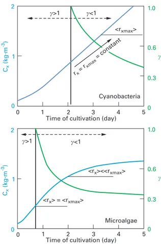
Figure 10.9 presents results for batch conditions, given here as a first illustra-tion. The illuminated fraction is also represented to emphasize the relation between light-attenuation conditions and resulting productivity. All results are given here for a constant PFD, assuming no limitation other than light. Thus, the time course of growth rate (<rx>) is explained here only by the changes in light

conditions in the culture volume due to biomass growth (no nutrient limitation). Because of their difference in photosynthetic response, microalgae and cyano-bacteria present different growth curves. In both cases, the kinetic regime (γ > l), usually encountered at the beginning of a batch production run, leads to a loss of efficiency, as illustrated here by a growth rate <r_x> below maximum <r_xmax> (values in batch mode are given by the slope of Cx(t); see Eq. (10.5)). This is explained by

light transmission, which prevents the full exploitation of the light energy received. Due to the increase in biomass, the γ value will decrease progressively to a value below 1. For prokaryotic cells (Fig. 10.9, left), as soon as full absorption is reached, the maximum value of the mean volumetric growth rate will be achieved and then remain constant (until a large dark zone is formed, inducing a shift in the cell metabolism, not represented here). For eukaryotic cells, the γ = 1 condition, giving the maximum value of the mean volumetric growth rate, will be only transiently satisfied. The increase in the dark volume will then progressively lower the mean volumetric growth rate (Fig. 10.9, right).

The same model can be applied to simulate continuous cultivation (by apply-ing only the appropriate formulation of the mass balance equation, i.e. τ ≠ 0 in Eq. (10.5)). In this case, a steady state is obtained for each set of operating condi-tions with constant biomass concentration and thus constant light-attenuation con-ditions. An example of the results is given in Figure 10.10 for C. reinhardtii growth.

Fig. 10.9: Time course of biomass concentration during a batch cultivation of Arthrospira

platen-sis (cyanobacteria, left) and Chlamydomonas reinhardtii (microalgae, right) (light-limited

condi-tions). Light attenuation increases with biomass concentration, directly affecting growth kinetics (slope of the curve). This proves to depend entirely on the illuminated fraction γ. We note that due to their respiration activity, microalgae are affected negatively by the formation and expan-sion of the dark zone (γ < 1).

The model was found to be accurate over the wide range of PFD investigated (up to 1000 µmol.m–2_.s–1_{), and for any light-attenuation conditions as obtained by}

varying the residence time τ and thus biomass concentration. Results are given here for the luminostat regime with γ = 1 giving maximum biomass productivity, and for full-light absorption with γ = 0.5. Accurate predictions were also obtained in kinetic regime γ > 1; see Takache et al. (2012).

Another example is given to illustrate the utility of modeling in PBR engineer-ing. Figure 10.11 presents the results obtained here with the green microalga

Neo-chloris oleoabundans cultivated in different PBRs (volume, culture depth) and

oper-ating conditions (PFD, residence time). The effects of all of these parameters were accurately predicted. Modeling thus emerges as a highly valuable tool in PBR

engi-Fig. 10.10: Prediction of PFD influence on resulting biomass productivity (continuous mode)

calcu-lated by the model presented. Comparison with experimental results for the green microalga

Chlamydomonas reinhardtii cultivated in a torus-shaped PBR (Lz= 0.04 m). The negative influence of introducing a dark volume on microalgal growth is illustrated here, with lower productivities when working in full-light absorption (γ = 0.5) than in the case of a luminostat regime (γ = 1) giv-ing maximal biomass productivity) (see Takache et al. 2012).

neering, enabling us to predict the influence of parameters that affect PBR perform-ance profoundly but in a complex manner.

Figure 10.11 illustrates the utility of increasing the specific illuminated surface (or decreasing the culture depth, i.e. alight= 1 / L for a flat panel) and PFD to

increase volumetric productivity (or biomass concentration, the two being linked). This introduces the basic concepts of PBR intensification, detailed in Fig. 10.12. The utility of working in a thin film (alight> 100 m–1, L < 0.01 m) is clearly

demon-strated here: compared with usual geometries (a_light around 20 m–1 _{for PBR of}

depth 0.05 m, 0.3 m–1 _{for raceway of depth 0.3 m), two orders of magnitude on}

volumetric productivity can be gained allowing operators to work in high cell den-sity culture (C_x> 10 kg.m–3_{). We also note that increasing the PFD will lead to a}

further increase (but with a decrease in thermodynamic yield, as discussed above). As previously mentioned, this demonstrates the surface productivity as being inde-pendent of the specific illuminated surface, emphasizing a specific feature of PBR intensification with the possibility to increase drastically volumetric productivity while maintaining surface productivity (see also Eq. (10.31) combined with Eq. (10.32)).

Generally, one direct utility of process intensification is that it reduces the system size needed to achieve a given production requirement. In the specific con-text of microalgal cultivation, we also note that several processes have an energy consumption directly linked to the culture volume (pumping, mixing, temperature control, harvesting, etc.). Increasing volumetric productivity can thus drastically

Fig. 10.11: Scaling up of biomass production from laboratory scale 1 L PBR to 130 L PBR with

Neo-chloris oleoabundans. The light-limited growth model was used to predict effects of different

parameters on productivities or biomass concentration (dashed line for PBR1 and continuous line for PBR2), such as the positive effect of increasing the PFD on biomass productivity, or the nega-tive effect of increasing the depth of culture.

reduce energy needs for a given operation. This is of primary relevance, for exam-ple, in biofuel production, where both surface and volumetric productivities can be increased with appropriate engineering of photobioreactors (using, for example, models described in this chapter; the authors are developing optimized systems for solar production by these means).

Fig. 10.12: Influence of the illuminated surface-to-volume ratio (alight) on PBR productivities in the

case of Chlamydomonas reinhardtii cultivation. A direct influence on volumetric productivity is shown (two orders of magnitude of variation). Surface productivity is found independent of this engineering parameter. PFD is found to have a positive effect on both values (all values corre-spond to maximal performances as obtained in continuous cultivation, light-limited conditions, luminostat “γ = 1” regime).

10.4.1.4 Engineering formula for assessment of maximum kinetic performance in PBRs

Among the many practical advantages of defining an illuminated volume fraction

γ in the PBR, we note that it enables us to clearly define (at least from a didactic

and theoretical point of view) optimal operating conditions for a given geometry of a PBR illuminated with a constant PFD. This means that from a sound control of the radiation field by acting on the biomass concentration guaranteeing the condition γ = 1 as rigorously as possible, it is possible to achieve the maximal kinetic performance of the PBR <rX>max. This also shows that for an existing reactor

and fixed PFD, the radiation field may be controlled solely by the biomass concen-tration CX(varying the residence time as previously shown), demonstrating why

batch cultivations for microalgae should be avoided if maximal performance is sought.

The authors have recently shown (Cornet and Dussap 2009), on many different PBR geometries, that only in the special case γ = 1 ± 20 %, and accepting an accu-racy of around 15 %, is it possible to use a simple engineering formula, already averaged over the total volume of the PBR, in which the complexity of the radiative

transfer has vanished. This very useful relation, with for main parameters the design-specific illuminated area alight and the incident PFD q0 (here in

μmolhν.m–2.s–1) with its degree of collimation n, takes the form:

< rX>max= (1 − fd) ρMMX¯φ′X 2α 1 + αalight K

(

)

[

(

)

]

in which all the variables have already been defined in this chapter except for fd,

which represents the dark fraction of the reactor (any volume fraction of the PBR not lit by the incident PFD). In this equation, the only specific parameters of a given micro-organism are the linear scattering modulus α (default value 0.9), the molar mass MX (default value 0.024 kgX/molX) and the half saturation constant

for photosynthesis K (default value 100 μmolhν.m–2.s–1). This formula, originally

validated for cyanobacteria, also proved very robust for microalgae (Takache et al. 2010).

10.4.2 Solar production

10.4.2.1 Prediction of PBR productivity as a function of radiation conditions

Generally, in the current perspective of using mass scale production of algae as a new feedstock source for various applications, predicting productivity is obviously useful (productivity calculations, cultivation system engineering, advanced control settings, etc.). However, the broad variability of sunlight in time and space adds further complexity to the optimization and control of cultivation systems, com-pared with artificial illumination. Modeling can be very helpful in this regard, and the approach was recently extended by the authors to that end by considering specific features of solar use such as (1) direct/diffuse radiation proportions in sunlight, and (2) time variation of the incident light flux and corresponding inci-dent angle on the surface of the cultivation system. All these variables can be obtained from a solar database giving time (day/night, season) and space variabil-ity of solar radiation. They can then be implemented in a PBR model, using the same approach as described above. Besides the specific nature of sunlight (non-normal incident angle, non-negligible diffuse radiation), an important difference lies in the transient nature of sunlight. The transient form of the mass balance equation thus has to be solved (this can be achieved using the routine ode23tb in the Matlab® _{software), ultimately allowing the determination of the biomass}

concentration time course and calculation of the corresponding biomass productiv-ity.

Once the model has been set up, it enables us to link various interacting parameters (irradiation, PBR technology and implementation) and phenomena