Towards deadlock free Sokoban
Tristan Cazenave1 and Nicolas Jouandeau21 LAMSADE, Universit´e Paris-Dauphine, Place Mar´echal de Lattre de Tassigny,
75775 Paris Cedex 16, France email: cazenave@lamsade.dauphine.fr
2 Universit´e Paris 8, LIASD, 2 rue de la libert´e, 93526, Saint-Denis, France
email: n@ai.univ-paris8.fr
Abstract. We present algorithms to compute and match maze specific deadlock tables at Sokoban. They enable to use a greedy search that can solve problems that are not solvable using IDA*.
1
Introduction
Sokoban is a PSPACE-complete single agent search problem [3]. The presence of deadlocks makes Sokoban hard to solve even non optimally. Identifying deadlock states is therefore an important step towards solving Sokoban. In this paper we describe algorithms that find maze specific deadlocks as well as efficient algo-rithms to match the deadlocks during search.
The second section details deadlocks, the third section explains how they can be efficiently matched, the fourth section deals with the retrograde analysis of deadlocks, the fifth section deals with search algorithm using deadlocks, the sixth section gives experimental results.
2
Maze specific deadlocks
In Rolling Stone [8, 6, 7] small 5x4 deadlock patterns are used to find simple deadlocks. Moreover a specific search algorithm is used to identifiy conflict among limited subsets of stones and dynamically create penalty patterns.
We use a different approach since we compute maze specific deadlocks con-taining a predefined number of stones.
Basic one stone and two stones deadlocks can be defined as:
– stones in corners,
– stones on a border between two corners, – two adjoining stones along a wall.
More complex deadlocks are computed using retrograde analysis. Retrograde analysis has already been successfully used in two player [13, 11, 14, 1, 2, 12] and single agent games [9, 4, 10, 5].
3
Forest of deadlocks
A deadlock is represented as an ordered set of locations of stones followed by a location of the man. Two deadlocks can have the same locations of stones and a different location for the man.
We represent sets of deadlocks as a different forest for each maze. Each tree of the forest is rooted at a location of the maze, the deadlocks in the tree all contains a stone at that location. The children of the root contain the different second locations of deadlock in the set of deadlocks starting at the root, and so on.
A deadlock can be matched on a screen if a subset of all the stones in the screen corresponds to the set of stones of the deadlock and if the man on the screen can see the man of the deadlock inside the deadlock screen.
In order to verify all deadlocks for a screen, the tree associated to each stone in the screen is verified. The verification consists in checking recursively for each child that the corresponding stone is present in the screen.
The next figures explain how a tree is built for three deadlock with the same first location. ##### ##### ##### #@ # #@ # # # # # # # # # ### ## ### ## ### ## # # # # # # ### #$## # ###### ### #$## # ###### ### #$## # ###### # #$## ##### ..# # # ## ##### ..# # # ## ##### ..# # ..# # $ $ ..# # $ $ ..# ##### ### # ## ..# ##### ### # ## ..# #####@### # ## ..# # ######### # ######### # ######### ####### ####### ####### 16 21 (0) 16 29 32 (0) 21 (0) 16 29 33 (44) 32 (0) 21 (0)
The first screen is a two stones deadlock containing locations 16 and 21 and the man at location 0. These two locations and the location of the man are used to build the leftmost tree. Then the second deadlock containing locations 16, 29 and 32 and the man at location 0 is added to the tree, resulting in the tree in the middle. The third deadlock (16, 29, 33 and man at 44) is then added and gives the rightmost tree.
Nodes contain a stone and possibly several man locations. The pseudo-code for verifying a tree is:
deadlock tree verification process
bool known_state (deadlock, man) if stone in state
for deadlockMan in men
if deadlockMan can see man in deadlock return true
push stone in deadlock for c in children
if c->known_state (deadlock, man) return true
pop stone from deadlock return false
A state is a maze containing stones at different locations and a man at a given location, the goal of the tree verification is to find if a subset of the stones of a state, is a deadlock. At each node of the tree, the algorithm verifies that the state contains the stone of the node. If a node contains deadlocks, it contains men locations. If one of the men locations is visible from the man in the state, a deadlock is found. Otherwise the verification continues for all children of the node.
All the trees rooted to the locations of the stones of a state are verified.
4
Retrograde analysis of deadlocks
Retrograde analysis starts with finding all the possible combinations of three stones. In a first pass, for each combination, it verifies that a subset is not already a deadlock. Then it tries all possible moves and verifies that they all lead to a known deadlock. When it is the case the combination is added to the set of deadlocks. In the subsequent passes, it goes through all the found deadlocks, finds all possible previous states. For each previous state, it checks if all moves lead to a known deadlock, and when it is the case the previous state is added to the set of deadlocks.
The pseudo code for the first pass is:
Combinations deadlock search process
list combinationsDeadlocksSearch (nbStones) list = empty list
state = first_combination (nbStones) while true
if state is not a known deadlock isDeadlock = 1
if child is not a known deadlock isDeadlock = 0
break
if isDeadlock equals 1 add state to deadlocksTree push state in list
if state equals last_combination (nbStones) break
state = next_combination (state) return list
The pseudo code for subsequent passes is:
Subsequent passes deadlock search process
list subsequentDeadlocksSearch (nbStones, states) list = empty_list
for state in states
for move in possiblePreviousMoves (state) parent = apply (state, move)
if parent is not a known deadlock isDeadlock = 1
for child in nextStates (parent) if child is not a known deadlock
isDeadlock = 0 break
if isDeadlock equals 1
add parent to deadlocksTree add parent to list
return list
Finding all possible combinations in the first pass can be time consuming when the number of stones grows. Many possible combinations do not lead to a deadlock, moreover a first pass deadlock is often a state where a move leads to a smaller deadlock. In order to rapidly compute the first pass, we only consider states where a move leads to a smaller deadlock. These states can be efficiently found by taking a smaller deadlock, finding all previous states, and adding the missing stones in every possible location.
The pseudo code for the first pass using the smaller deadlocks is:
Smaller deadlock search process
list smallerDeadlocksSearch (nbStones) list = empty list
for P = 1; P < nbStones && P <= Pmax; P++ previous_states = empty list
for deadlock in deadlocksTree with nbStones-P stones push deadlock in previous_states
for state in previous_states
for move in possiblePreviousMoves (state) parent = apply (state, move)
freeStates = free_states (parent)
subState = first_combination (P, freeStates) while true
newState = parent + subState
if newState is not a known deadlock isDeadlock = 1
for child in nextStates (newState) if child is not a known deadlock
isDeadlock = 0 break
if isDeadlock equals 1
add newState to deadlocksTree push newState in list
if subState equals last_combination (P, freeStates) break
subState = next_combination (subState, freeStates) return list
However the first pass using the smaller deadlock does not find all possible deadlocks. For example a few deadlocks do not have any possible moves and are not found by the smaller deadlock search.
Here are some examples of deadlocks that are not found:
############ ######## ######## #..@ # ### #@ # #@ # #.. # # # # ## # # ## #.. # #### # # # # # #.. ## # ##$ # ##$ # #.. # # $$## ######### $$#$### ######### $$# ### ######$##$ $ # #.... ## $ $ # #.... ## $ $ # # $ $ # ##... # ##... $ # # # # #.... ########## #.... ########## ############ ######## ########
Only very few deadlocks have no possible moves. However the algorithm also misses other deadlocks that are based on even smaller deadlocks that the one used.
The retrograde analysis algorithm we have used starts its first passes with all possible combinations of stones until a predefined number of stones (maxS-tonesCombination), and then continues with first passes based on smaller dead-locks:
Global deadlock search process
nbStones = 1
while not end of deadlock search if nbStones < maxStonesCombination
newStates = combinationsDeadlocksSearch (nbStones) else
newStates = smallerDeadlocksSearch (nbStones) while size of newStates is not 0
otherStates = subsequentDeadlocksSearch (nbStones, newStates) newStates = otherStates
nbStones++
Another way of looking at Sokoban problems is to start from the goal position and going backward to the start position pulling stones. In this case, the usual deadlocks never appear since the goal position is always reachable by pushing back stones. However other kinds of deadlocks appears which stop the backward search: the pull deadlocks.
Here are example of one stone, two stones and 6 stones pull deadlocks for screens 1 and 13: ##### ##### ######### #@ # # # ## ## ##### # # # # ###@$$ # # ### ### ## ### ## # $ # # # ... # # # #@ $ # # # #$$## # #.#. # ### # ## # ###### ### # ## # ###### # # # # . . # # # ## ##### ..# # $# ## ##### ..# # $ # # #.#. # # ..# # ..# # ## ## . . # ##### ###$# ## ..# ##### ### # ## ..# # # # # #.#. # # ######### # ######### ## ... # ####### ####### # ###### ## # # # ########## ####
In the first one stone pull deadlock, the stone cannot be pulled. In the second two stones pull deadlock pulling the stones reaches a position where no more pulling moves are possible. In the last six stone pull deadlock a more complex retrograde analysis finds that all moves lead to position where no more moves are available, and the man is trapped in a local area.
5
Searching with deadlocks
In this section, we present the algorithms we use to solve problems. The first algorithm is a greedy search. It consists in developping the state that has the minimal associated heuristic. A greedy search is pointless in Sokoban without
deadlock verification since it is trapped in promising deadlock states for a very long time. When deadlocks can be detected a greedy search avoids such states and can find solutions.
The pseudo code for the greedy algorithm with deadlock verification is:
Greedy algorithm
void greedy (initialState)
currentGreedy = manhattan (initialState)
push initialState in sortedStates [currentGreedy] while not end of search
while size of sortedStates [currentGreedy] is 0 currentGreedy ++
state = front of sortedStates [currentGreedy] pop front of sortedStates [currentGreedy] for child in nextStates (state)
if child is without remaining stones return
if child is known as deadlock continue
h = manhattan (child)
push child in front of sortedStates [h] if h < currentGreedy
currentGreedy = h
The other algorithm we have tested is IDA*. We used a very simple admissible heuristic which consists in summing for all stones the distance to the closest goal location. Moreover we do not place stones inside the goal area and assume they are at their goal location as soon as they enter the area.
The greedy algorithm is very similar for pull deadlocks, except that the heuristic used is a greedy one, the closest pair of stone and start location is chosen, their distance is added to the heuristic, then the start location is re-moved from the possible locations and the process is repeated until all pairs have been chosen.
6
Results
In order to compute the deadlock tables, all combinations are tried until 4 stones, then for more stones, a smaller search first pass with P max = 2 is performed, followed by usual passes. Table 1 gives the time used to build deadlock tables and the number of deadlocks found for screen 13. A distinction is made between the first pass and subsequent passes. For 5 stones, the combination search takes 40 minutes and the smaller search takes 10 seconds, the number of deadlock found in the first pass of the smaller search is higher than in the combination search since it the order in which it considers deadlocks is not the same and as it checks a deadlock as soon as it is found. For 10 stones, the smaller search uses 2h14m for the first pass and 1 minute for subsequent passes.
Table 1. Time needed and number of deadlocks found with deadlock search. screen 13 with combination with smaller P max = 2
time nb passes 1st next time nb passes 1st next
1 <1s 2 40 0 2 <1s 4 49 6 3 1s 5 59 20 4 40s 6 160 117 5 40m 7 417 345 10s 6 440 244 6 43s 8 1576 1057 7 2m16s 7 4075 3042 8 9m47s 8 12970 10534 9 33m31s 10 38775 36838 10 2h15m 11 154480 132908 11 8h33m 11 411582 300621 12 33h20m 17 603892 403528
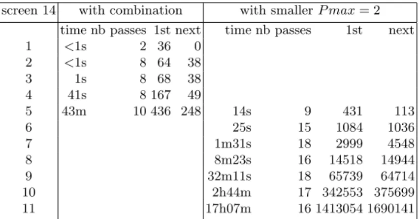
Table 2. Time needed and number of deadlocks found with deadlock search. screen 14 with combination with smaller P max = 2
time nb passes 1st next time nb passes 1st next
1 <1s 2 36 0 2 <1s 8 64 38 3 1s 8 68 38 4 41s 8 167 49 5 43m 10 436 248 14s 9 431 113 6 25s 15 1084 1036 7 1m31s 18 2999 4548 8 8m23s 16 14518 14944 9 32m11s 18 65739 64714 10 2h44m 17 342553 375699 11 17h07m 16 1413054 1690141
Table 2 gives similar information for the deadlocks of screen 14.
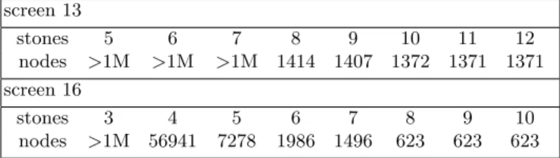
Table 3 gives the number of nodes required to solve screen 13 and screen 16 with a greedy search and different deadlock tables. Using deadlock tables with only three stones it does not solve the problem 16 in one million nodes. Using four stones deadlock tables, it solves screen 16 in 56941 nodes. The number of nodes decreases with the number of deadlock stones until 8 where it reaches its minimum at 623 nodes. Concerning screen 13, the problem can be solved with the 8 stones deadlock tables, computing more deadlock tables is of little practical interest given the computing times of the deadlock tables greater than 8 stones given in table 1.
Table 3. Greedy search with different numbers of deadlock tables. screen 13 stones 5 6 7 8 9 10 11 12 nodes >1M >1M >1M 1414 1407 1372 1371 1371 screen 16 stones 3 4 5 6 7 8 9 10 nodes >1M 56941 7278 1986 1496 623 623 623
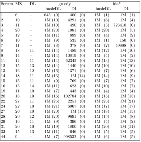
Table 4 compares the different search algorithms on different screens. The greedy algorithm with deadlock tables solves most of the problems we have tested. It solves problems 13, 15, 16, 18, 20, 22, 24, 28, 29, 31, 32 and 44 which are not solved by Rolling Stone. The first column of the table is the number of the screen, the second column is the number of stones of the screen, the third column gives the number of deadlock stones in the tables (– if equals to the number of stones), the fourth column gives the number of nodes used by a greedy search without deadlock tables (search is stopped after 1M nodes, so 1M means the search has failed), the fifth column gives the number of remaining stones for the position in the greedy search that has the minimum such number, the sixth colmun give the number of nodes used by a greedy search with deadlock tables, the seventh column the related number of remaining stones, the seventh column the number of nodes of IDA* without deadlock tables, the eight column the related number of remaining stones, the ninth column the number of nodes of IDA* with deadlock tables and the last column the related number of remaining stones.
Our current greedy search does not manage the placement of the stones in the goal area, as soon as a stone is in the goal area it is removed and considered as placed in the right location of the goal area. For many problems this simpli-fication does not change the solution of the problem, however in some screens there can be interactions between the goal area and the solution or there can be multiple goal areas (for example in screen 18 there are three goal areas so our solution is not valid, in screen 15 there are two stones in the goal areas in the start position and they interact with the solution so our greedy solution is also not valid). Our simplification poses no problem in screens with a simple goal area such as screens 13, 20, 24, 28 and 31 which are solved by greedy search with deadlock tables and not by Rolling Stone.
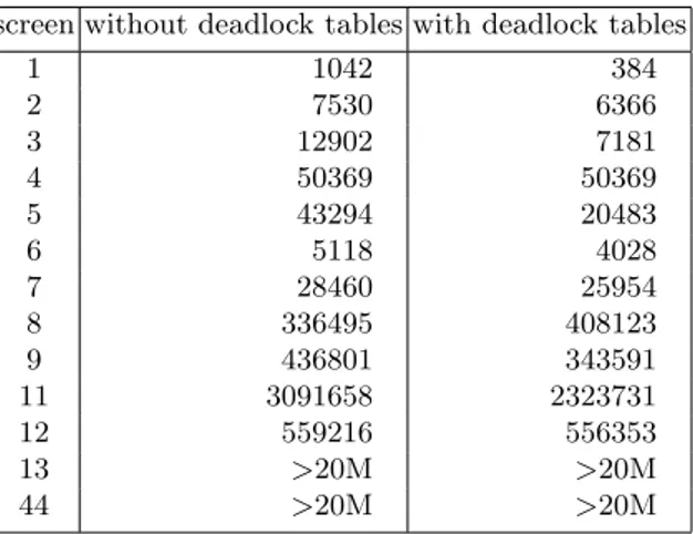
Deadlock tables were added to Rolling Stone. The IDA* search was stopped as soon as a deadlock was encountered. The results are given in table 5. The first column gives the screen number, the second column gives the number of nodes used by the original Rolling Stone, the third column gives the number of nodes used by Rolling Stone equipped with deadlock tables. Deadlock tables reduce the number of nodes for almost all problems, problem 8 being an exception. A
possible explanation is that in this problem some penalty patterns could not be found by Rolling Stone due to deadlock tables cuts and could not be reused in other parts of the search.
Table 6 gives the number of pull deadlocks and their computation times for screen 13.
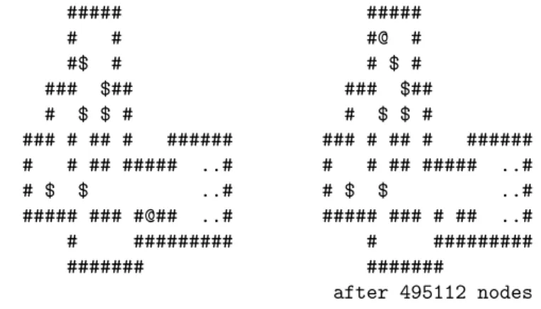
A greedy search with pull deadlocks can be trapped in position that are close to the goal position but that are not solvable. Here is an example for screen 1 where the search is one move away from the start but is in a hopeless position, moreover the man cannot move to its start position:
##### ##### # # #@ # #$ # # $ # ### $## ### $## # $ $ # # $ $ # ### # ## # ###### ### # ## # ###### # # ## ##### ..# # # ## ##### ..# # $ $ ..# # $ $ ..# ##### ### #@## ..# ##### ### # ## ..# # ######### # ######### ####### ####### after 495112 nodes
7
Conclusion
We have presented how to use retrograde analysis to compute maze specific deadlock tables at Sokoban, we have also presented how to use deadlock trees to match the computed deadlocks efficiently as well as a greedy search algorithm. Moreover we have presented a new way to solve Sokoban problems pulling stones out from the goal area towards their start positions as well as the related pull deadlocks.
These algorithms have been tested on many Sokoban screens including diffi-cult ones. Computing maze specific deadlock tables has enabled to successfully use a greedy search at Sokoban and to solve problems that are not solved by IDA*.
In future works, we will improve greedy search so as to cope with the place-ment of stones in the goal area. We will also try to improve the retrograde analysis efficiency and completeness.
References
1. T. Cazenave. Automatic Acquisition of Tactical Go Rules. In Game Programming
Table 4. Number of nodes evaluated and resulting top level node needed to solve problems.
Screen MZ DL greedy ida*
basicDL DL basicDL DL 1 6 – 643 (0) 400 (0) 1M (1) 1M (1) 2 10 – 1M (10) 4291 (0) 1M (6) 1M (4) 3 11 – 1M (10) 490 (0) 1M (3) 723410 (0) 4 20 – 1M (20) 1981 (0) 1M (20) 1M (5) 5 12 – 1M (11) 899 (0) 1M (4) 1M (2) 6 10 – 1M (9) 535 (0) 1M (1) 150 (0) 7 11 – 1M (8) 378 (0) 1M (2) 40888 (0) 8 18 11 1M (14) 1489 (0) 1M (12) 1M (10) 9 14 – 1M (14) 10819 (0) 1M (4) 1M (2) 11 14 11 1M (14) 62345 (0) 1M (13) 1M (13) 12 15 13 1M (14) 1440 (0) 1M (10) 1M (10) 13 16 12 1M (16) 1371 (0) 1M (7) 1M (6) 14 18 11 1M (13) 1M (14) 1M (14) 1M (9) 15 15 11 1M (9) 769 (0) 1M (7) 1M (7) 16 15 14 1M (11) 623 (0) 1M (10) 1M (7) 18 11 10 1M (7) 443 (0) 1M (4) 1M (4) 20 18 10 1M (16) 102784 (0) 1M (15) 1M (15) 22 27 11 1M (25) 2251 (0) 1M (25) 1M (21) 24 22 10 1M (21) 6967 (0) 1M (17) 1M (17) 27 20 10 1M (20) 1M (15) 1M (18) 1M (15) 28 20 12 1M (20) 9691 (0) 1M (15) 1M (8) 29 16 11 1M (9) 396 (0) 1M (4) 1M (2) 31 20 10 1M (19) 1800 (0) 1M (20) 1M (11) 32 15 13 1M (11) 646 (0) 1M (5) 1M (5) 44 9 – 1M (7) 908532 (0) 1M (6) 1M (5)
2. T. Cazenave. Generation of Patterns With External Conditions for the Game of Go. In H.J. van den Herik and B. Monien, editors, Advances in Computer Games
9, pages 275–293. Universiteit Maastricht, Maastricht, 2001.
3. J. C. Culberson. Sokoban is PSPACE-complete. In L. Pagli E. Lodi and N. Santoro, editors, Conference on Fun With Algorithms, pages 65–76, Waterloo, 1999. Carleton Scientific.
4. J. C. Culberson and J. Schaeffer. Pattern Databases. Computational Intelligence, 4(14):318–334, 1998.
5. A. Felner, R. E. Korf, R. Meshulam, and R. C. Holte. Compressed pattern databases. J. Artif. Intell. Res. (JAIR), 30:213–247, 2007.
6. A. Junghanns. Pushing the limits: New developments in single-agent search. Phd thesis, University of Alberta, 1999.
7. A. Junghanns and J. Schaeffer. Sokoban: Enhancing general single-agent search methods using domain knowledge. Artif. Intell., 129(1-2):219–251, 2001.
Table 5. Total nodes searched with Rolling Stone. screen without deadlock tables with deadlock tables
1 1042 384 2 7530 6366 3 12902 7181 4 50369 50369 5 43294 20483 6 5118 4028 7 28460 25954 8 336495 408123 9 436801 343591 11 3091658 2323731 12 559216 556353 13 >20M >20M 44 >20M >20M
Table 6. Time needed and number of pull deadlocks found with pull deadlock search. screen 13 with combination with smaller P max = 2
time nb passes 1st next time nb passes 1st next
1 <1s 1 0 – 2 <1s 3 35 2 3 8s 2 78 0 4 10m51s 2 234 0 5 16s 10 195 400 6 76s 10 714 1023
Theor. Comput. Sci., 252(1-2):151–175, 2001.
9. R. E. Korf. Finding optimal solutions to rubik’s cube using pattern databases. In
AAAI-97, pages 700–705, 1997.
10. R. E. Korf and A. Felner. Disjoint pattern database heuristics. Artificial
Intelli-gence, 134(1-2):9–22, 2002.
11. R. Lake, J. Schaeffer, and P. Lu. Solving large retrograde-analysis problems using a network of workstations. In H.J. van den Herik, I.S. Herschberg, and J.W.H.M. Uiterwijk, editors, Advances in Computer Chess 7, pages 135–162. University of Limburg, Maastricht, The Netherlands, 1994.
12. J. W. Romein and H. E. Bal. Solving awari with parallel retrograde analysis. IEEE
Computer, 36(10):26–33, October 2003.
13. K. Thompson. Retrograde analysis of certain endgames. ICCA Journal, 9(3):131– 139, 1986.