SPATIAL AND TEJVIPORAL VARIATIONS IN CLIMATE TRENDS FROM BOREHOLE TEMPERATURE DATA
DISSERTATION PRESE TED
AS PARTIAL REQUIREMENT
OF THE DOCTORATE OF ENVIRONMENTAL SCIENCES
BY
CAROLYNE PICKLER
Avertissement
La diffusion de cette thèse se fait dans le respect des droits de son auteur, qui a signé le formulaire Autorisation de reproduire et de diffuser un travail de recherche de cycles supérieurs (SDU-522 - Rév.0?-2011 ). Cette autorisation stipule que «conformément à l'article 11 du Règlement no 8 des études de cycles supérieurs, [l'auteur] concède à l'Université du Québec à Montréal une licence non exclusive d'utilisation et de publication de la totalité ou d'une partie importante de [son] travail de recherche pour des fins pédagogiques et non commerciales. Plus précisément, [l'auteur] autorise l'Université du Québec à Montréal à reproduire, diffuser, prêter, distribuer ou vendre des copies de [son] travail de recherche à des fins non commerciales sur quelque support que ce soit, y compris l'Internet. Cette licence et cette autorisation n'entraînent pas une renonciation de [la] part [de l'auteur] à [ses] droits moraux ni à [ses] droits de propriété intellectuelle. Sauf entente contraire, [l'auteur] conserve la liberté de diffuser et de commercialiser ou non ce travail dont [il] possède un exemplaire.»
VARIATIONS SPATIALES ET TEMPORELLES DES TENDANCES
CLIMATIQUES DÉDUITES DES PROFILS DE TEMPÉRATURE DU
SOUS-SOL
THÈSE
PRÉSENTÉE
COMME EXIGENCE PARTIELLE
DU DOCTORAT EN SCIENCES DE L'ENVIRO NEME T
PAR
CAROLYNE PICKLER
The works presented in this dissertation represent the blood, sweat, and tears of thr e plus years of work. I would like to thank my supervisors, Dr. Hugo Beltrami and Dr. Jean-Claude Mareschal, for giving me the opportunity to undertake this adventure. From field work to analysis to article writing and reviewing, I have learnt so much from bath of you. Furthemore, I would like to thank the UQAM Faculty of Science, NSERC and the SERC-CREATE Training program in Cli-mate Science based at St. Francis Xavier University for the financial support.
The geophysics lab has also been a huge source of motivation throughout this endeavour. They have motivated me, distracted me and forced me to watch the horrible sloth short. A big thanks to the geophysics crew: Jean-Claude, Fiona, Lidia, Ignacio, Dr. Francesco Fish Geophysical Experim nt, Arlette (our honorary geophysicist) and Fernando. Without your friendship, support, dances, sarcastic comments, and food/liquor, I wouldn't have survived, let alone loved this exp eri-ence. A big thanks also to the SAQ, who provided the much needed libation for Friday afternoon geophysics parties.
Finally, I would like to thank my friends and family for their unconditional support and ability to put up with my craziness. Erica, thanks for listening to my rants and always understanding my klutzy moments. To my family, my parents, Andy, and Mr. Baby Bear, thanks for always cheering me on and the moral/immoral support. To my favourite Spaniard, Fernando, thanks for always making me laugh and smile and understanding every step of this crazy process.
This dissertation is presented as three scientific articles that have been co-authored by my supervisors, Dr. Hugo Beltrami and Dr. Jean-Claude Marcschal. The first article entitled Laurentide lee Sheet basal temperatures at the Last Glacial Cycle as inferred from borehole data has been published in Climate of the Past on 22 January 2016. The second article, Climate trends in northern Ontario and Quebec from borehole temperature profiles, has also been published in Climate of the Past on 16 December 2016. The third article is in preparation. The format of the published and submitted articles has be n modified to satisfy the presentation criteria for Université du Québec à Montréal dissertations.
LIST OF TABLES . LIST OF FIGURES
LIST OF ABBREVIATIONS A D ACRONYMS RÉSUMÉ ..
ABSTRACT INTRODUCTION
0.1 GST reconstructions from borehole temperature data 0.2 Measuring borehole temperature data . . . .
0.3 Suitability of borehole temperature data for climate studies . 0.4 Application of GST reconstructions . . . . vii lX xvii xviii xx 1 3 4 5 6 0.4.1 Basal temperatures of the Laurentide lee Sheet 6 0.4.2 Climate in northern Ontario and Québec for the past 500 years 7
0.4.3 Climate trends in northern Chile 8
0.5 Originality and contribution . . . . . . . 9 CHAPTER I
LAURENTIDE ICE SHEET BASAL TEMPERATURES AT THE LAST GLACIAL CYCLE AS INFERRED FROM BOREHOLE DATA . 11
1.1 Introduction . 13
1.2 Theory . . . . 17
1.2.1 First order stimate of the GST History 1.2.2 Inversion .. . .
1.2.3 Simultan ous inversion . 1.3 Data Description . .
1.4 Analysis and Results
18 19 20 21 23
1.4.1 Long-term Surface Temperatures 1.4.2 Individual inversions .. 1.4.3 Simultaneous Inversion . 23 24 28 1.5 Discussion . 29 1.6 Conclusions 31 CHAPTER II
CLIMATE TRENDS IN NORTHER ONTARIO AND QUÉBEC FROM
BOREHOLE TEMPERATURE PROFILES 46
2.1 Introduction . 48
2.2 Theory . . . . 52
2. 2.1 Inversion . 53
2.3 Description of data 54
2.4 Results . . . . . 56
2. 5 Discussion and Con cl usions 58
CHAPTER III
CLIMATE TRENDS FOR THE PAST 500 YEARS IN NORTHERN CHILE
FROM BOREHOLE TEMPERATURE DATA 75
3.1 Introduction . 77
3.2 Methodology 81
3. 2.1 Inversion .
3.2.2 Sinmltaneous inversion 3.3 Data description and selection . 3.4 Results ..
3.5 Discussion
3.5.1 Comparison hetween GST histories 3.5.2 Compari on with meteorological data . 3.5.3 Comparison with other climate proxies 3.5.4 CompariRon with models . . . .
83 84 84 87 88 88 89 90 91
3.6 Conclusions .. 92
3.6.1 El Loa . 94
3.6.2 Mansa 1t1ina . 94
3.6.3 Sierra Limon Verde . 95
3.6.4 Sierra Gorda 95
3.6.5 Vallenar 95
3.6.6 Copiap6 95
3.6.7 Tot oral 96
3.6.8 Punta Diaz 96
3.6.9 San José de Coquimbana . 96
CONCLUSION . .. . . . . . 115
APPENDIX A
GST RECONSTRUCTIONS FROM INVERSION OF THE TEMPERA-TURE ANOMALY . . . . . . . . . . . . . . . . . . . . . . . . . . . . . 120 APPENDIX B
INDIVIDUAL GST RECONSTRUCTIO S FOR NORTHERN 0 TARIO AND QUÉBEC . . . . . . . . . . . . . . . . . . . . . . . . . . . . 130 APPENDIX C
INDIVIDUAL GST RECONSTRUCTIONS FOR NORTHERN CHILE . 139 REFERENCES . . . . . . . . . . . . . . . . . . . . . . . . . 145
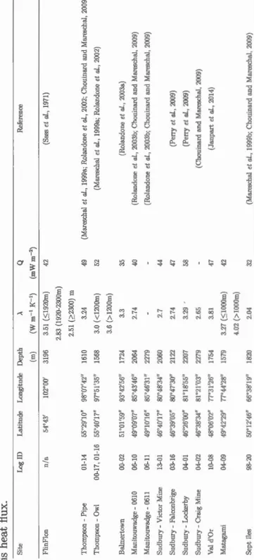
Table Pag 1.1 Technical information concerning the borehol s used in this study,
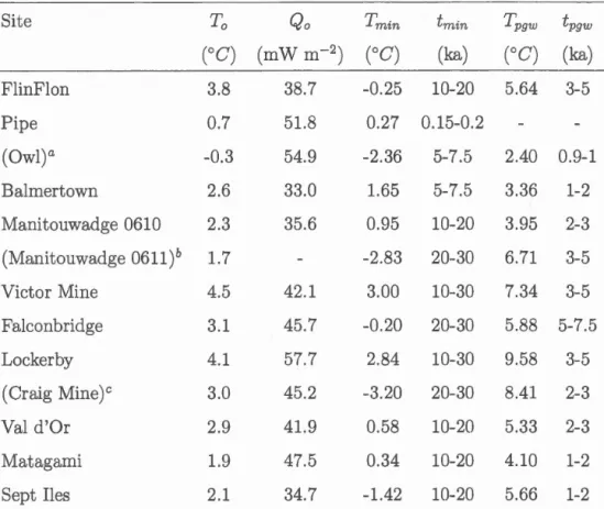
where À is thermal conductivity and Q is heat flux. . . . . . . . . 42 1.2 Summary of GST history results where Ta is the long-term
sur-face temperature, Qa is the quasi- quilibrium heat flow, Tmin is the minimal temperature, Tpgw is the maximum temperature attained during the po tglacial warming, tmin and tpgw is the occurr nee of the minimal temperature and maximum po tglacial warming tem-perature. Parentheses indicate sites where the GST history is not reliable. . . . . . . . . . . . . . . . . . . . . . . . . 43 1.3 Summary of GST history results for simultan ous inversions wh re
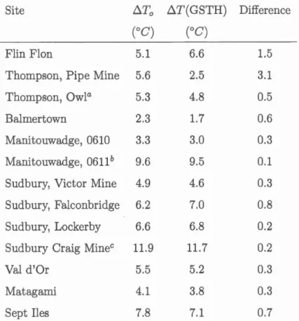
tmin and tpgw is the occurrenc of the minimal temperature and maximal temperature a sociated with postglacial warming, and 6.T is the temperature range . . . . . . . . . . . . . . . . . . . . . . . 44 1.4 Ranges in surface temperature variations stimated from: the it
r-ation of the long-tenn surface temperature as a function of depth (column 1) and from inversion of the GST history (column2), along with the difference between the two (column 3). . . . . . . . . . 45 2.1 Location and technical information concerning the borehol s used
in this study, where true depth is the depth corrected for the dip of the borehol , À is the thermal conductivity, Q is the heat flux, and Qcorr is the heat flux corrected for post glacial warming . . . 71 2.2 Location and technical information concering boreholes not sui table
for this study, where Ta is the reference surface temperature and Qa is th reference heat flux . . . . . . . . . . . . . . . . . . . . . 72 2.3 Summary GST History Results where Ta is th reference surface
temperatur , Qa is the r ference heat flux, 6.T is th difference betw en the maximal temperature and the reference temperature 500 years bcfore logging. . . . . . . . . . . . . . . . 73
2.4 Geological unit and rock type concerning th boreholes u ed in this study. . . . . . . . . . . . . . . . . . . . . . . . . . 74 3.1 Location and technical information concerning the borehole temperatur
e-depth profiles measured in 1994 by Springer (1997) and Springer and Forster (1998) . . . . . . . . . . . . . . . . . . . . . . . . . . 109 3.2 Location and technical information concerning the borehole t
emperature-depth profiles measured in 2012 by Gurza Fausto (2014) . . . . . 110 3.3 Location and technical information concerning the borehole tempera
ture-depth profiles measured in 2015 . . . . . . . . . . . . . . . . . . . 111 3.4 Technical information concerning boreholes not suitable for this study112 3.5 Summary of inversion results where Ta is the long-term surface
temperature, ra is the quasi-steady state temperature gradient and !::.. T is the difference betwcen the maximal temperature and th temperature at 1500 years CE. . . . . . . . . . . . . . . . 113 3.6 Summary of models used to calculat the multi-model mean surface
temperature anomaly from the PMIP3/C:f'v1IP5 simulation . . . . 114 A.1 Comparison of GST histories reconstructed from the temp rature
anomaly (anom) and the full profile (full) where Tmin(anom) is the minimum temp rature obtained by inverting the temperature anomaly, tmin(anom) is the timing of the minimal temperature ob-tained by inverting the temperature anomaly, Tmin(full) is th minimum t mperaturc obtained by inverting th full profile, and tmin(full) is the timing of the minimum temperature obtained from the inversion of the full profile. Parentheses indicate sites where the GST history is not reliable. . . . . . . . . . . . . . . . . . . . . . 129 B.1 Summary of GST results where Tais the long-term surface
temper-ature, qa is the quasi-steady state heat flux, f::.T is the difference between the maximal temperature and the refer nee temperature at 500 years BP. . . . . . . . . . . . . . . . . . . . . . . . . . 138
Figure
1.1 Map of central and eastern Canada and adjoining US showing the location of sampled boreholes. Thompson (Owl and Pipe), Man-itouwadge (0610 and 0611) and Sudbury (Falconbridge, Lockerby, Craig Mine, and Victor Mine) have several boreholes present within a small region. The number of profiles available at locations with
Page
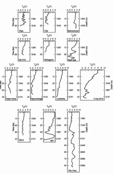
multiple hole is enclosed in parenthesis. . . . . . . . . . . . . 34 1.2 Heat flux variation as a function of depth. Heat flux is calculated
as th product of thermal conductivity by the temperature gradient calculated over 3 points. The Flin Flon, Owl and Matagami profil s have been corrected to account for thermal conductivity variations with depth as shown in Table 1.1. . . . . . . . . . . . . . 35 1.3 Long-term surface temperature variations over time (left y-axis)
and depth (right y-axis) for all the boreholes. Time is determined from depth by equation 1.7. . . . . . . . . . . . . . . . 36 1.4 Ground Surface Temperature History from the Manitoba boreholes,
at Flin Flon and Thompson (Pipe and Owl). The temperatures have been shifted with respect to the reference surface temperature of the site, Ta, as shown in Table 1.2. . . . . . . . . . . . . . . 37 1.5 Ground Surface Temperature History for the western Ontario
bore-hales: Balmertown and Manitouwadge 0610 and 0611. The tem-peratures have been shifted with respect to the reference surface temperature of the site, Ta, as shown in Table 1.2. . . . . . . . 38 1.6 Ground Surface Temperature History for all the borehol s around
Sudbury, Ontario (Victor Mine, Falconbridge, Lockerby, and Craig Min ) . The t mperatures have been shifted with respect to the ref -erence surface temperature of the site, Ta, as shown in Table 1.2. . 39 1.7 Ground Surface Temperature History for the boreholes in Quebec,
Matagami, Val d'Or and Sept-Iles. The temperatures have be n shifted with respect to the reference surface temperature of the site, Ta, as shown in Table 1.2. . . . . . . . . . . . . 40
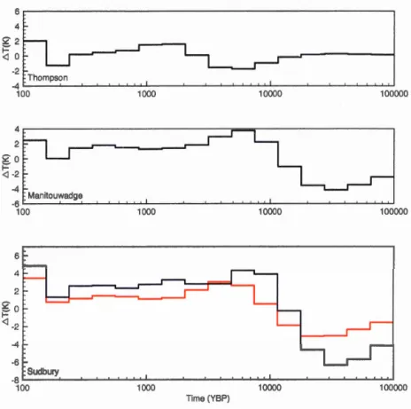
1.8 GST changes from simultaneous inversion with respect to the long-tenu temperature at 100 ka. The Sudbury GST changes include (black) and exclude (red) Craig Mine. . . . . . . . . . . . 41 2.1 Map of Ontario and western Québec showing the location of sites
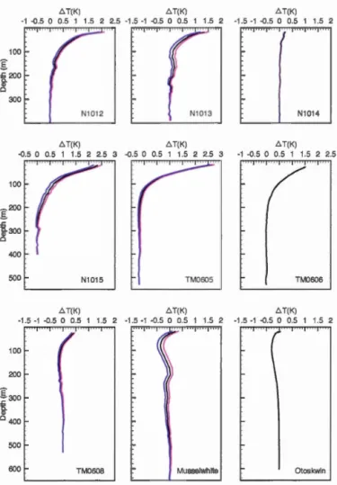
(red dots). For sites with several bor hol s (Camp Coulon , East-main, Thierry Min , and oro nt), the number of profiles available is enclosed in parenthesis. Black diamonds show the locations of sites that were discarded. . . . . . . . . . . . . . . . . . . 65 2.2 Temperature anomalies for the northern Ontario boreholes. Holes
TM0605, TIVI0606, and TM0608 are from the Thierry Mine site; holes N1012, N1013, N1014, and 1015 belong to th Noront site. The anomaly is obtained by subtracting the estimated steady-state geotherm obtain d by the least-squar fit of a straight line to the bottom 100 rn of the borehole temperature-depth profile. The black line represents the best linear fit, while the pink and blue lines are th upper and lower bounds, respectively, of the 2a confidence in-tervals. For N1014, TM0606, and Otoskwin, the upper and lower bounds of the confidence interval are not visible due to the temper
-ature scale. The temperature anomaly at l\1usselwhite was eut at 650 m. . . . . . . . . . . . . . . . . . . . . . . . . . . 66 2.3 Temperature anomalies for the northern Québec boreholes. CC0712,
CC0713, CC0714 are the boreholes from Camp Coulon; Ea0803 and Ea0804 are the boreholes from Eastmain . The anomaly is obtained by subtracting the estimated steady-state geotherm obtained by the least-square fit of a straight line to the bottom 100 rn of the borehole temperature-depth profile. The black line r presents the best linear fit, while the pink and blue lines represent the upper and lower bounds, respectively, of the 2a confidence intervals. The temperature anomaly at Nielsen Island was eut at 600m. . . . 67 2.4 GST histories for the northern Ontario sites determined by inver
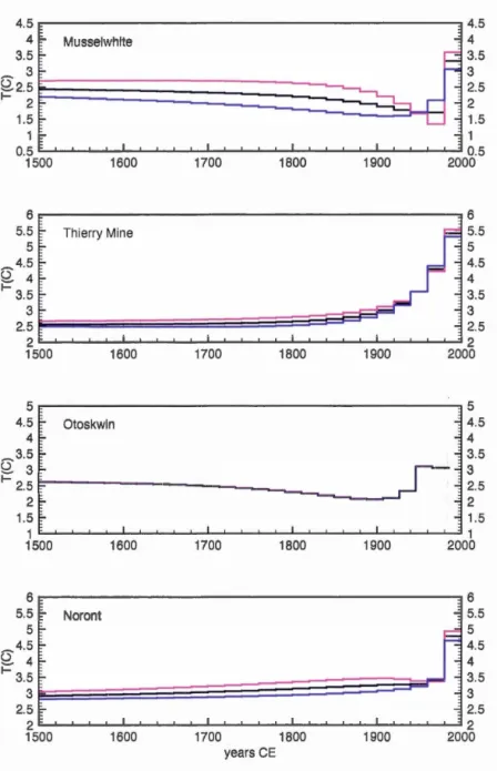
-sion of the anomalies. For multiple holes at a given site (Thierry Mine and Noront), simultaneous inversion was used. The pink and blue lines represent the inversions of the upper and lower bounds of the anomaly. For Otoskwin, the three lines are superposed. . . 68 2.5 GST histories for the northern Québec sites. Simultaneous
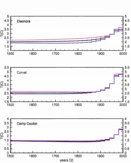
inver-sion was used for Eastmain, which includes two holes. The pink and blue lines represent the inversions of the upper and lower bounds of the anomaly. . . . . . . . . . . . . . . . . . . . . . . . . . . . . 69
2.6 GST histories for the northern Québec sites. Simultaneous inve
r-sion was used for Camp Coulon, which includes more than one hole.
The pink and blue lines represent the inversions of the upper and
lower bounds of the anomaly. . . . . . . . . . . . . . . . 70
3.1 Map of South America including locations of borehole temperature
measurements for heat flow studies (Lucazeau, personal
communi-cation). Red diamonds represents boreholes deeper than 200 rn,
while black are boreholes shallower than 200 m. More than 100
bottom-hole temperature measurements, mainly in Brazil, are not
includ d as they are not useful for climate studies. The rectangle
indicates the study region of northern Chile. . . . . . . . . . . 98
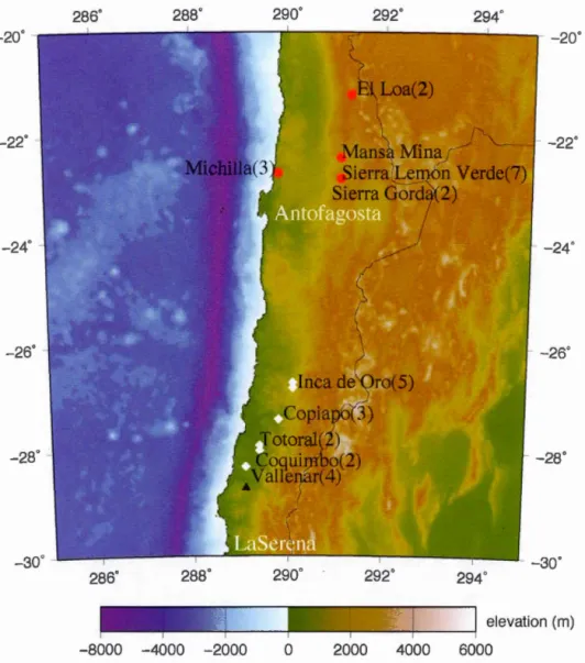
3.2 Map of northern Chile with locations of boreholes used in this study.
The number of boreholes at each site is indicated in parenthesis.
Red circles indicate borehole temperature-depth profil s measured
in 1994, black triangles are measured in 2012, and white diamonds
are measured in 2015. Sites with borehole temperature-depth
pro-files deemed suitable for climate are Michilla, Totoral, Inca de Oro,
and Vallenar. . . . . . . . . . . . . . . . . 99
3.3 Retained temperature-depth profiles measured in 1994 (green), 2012
(blue), and 2015 (pink). Temperature scale is shifted as indicated
in parenthesis. . . . . . . . . . . . . . . . . . . . . . . . 100
3.4 Temperature anomalies for the retained temperature-depth profiles,
where IDO is Inca de Oro. The pink and blue lines represent the
upper and lower bounds of the temperature anomaly. Th se are
not visible at IDO-DDH2457 and Vallenar ala1110-2 because they
are superimposed. . . . . . . . . . . . . . . . . . . . . . 101
3.5 GST history for northern coastal Chile (Michilla) detennined for
its period of measurement (1994) from the simultaneous inversion
of na12, p398, and z197, where 3 eigenvalues are r tained. The
pink and blue lines represent the inversion of the upper and lower
bounds of the temperature anomaly or the extremal steady states. 102
3.6 GST history for Inca de Oro determined from the simultan ous
inversion of DDH2457, 1501, 1504, and 1505, with 3 eig nvalues
retained. The pink and blue lines represent the inversion of the
up-per and lower bounds of the temperature anomaly or the extr mal
3.7 GST history for Totoral (RC370), with 3 eigenvalues retained. The pink and blue lines represent the inversion of the upper and lower bounds of the temperature anomaly or the extremal steady states. 103 3.8 GST history for Vallenar (ala1110-2), with 3 eigenvalues retained.
The inversion of the upper and lower bounds of the temperature anomaly or the extremal steady states are not visibl bccause the three lines are superimposed. . . . . . . . . . . . . . . . . . . 103 3.9 GST history for north-central Chile determined by the simult
ane-ous inversion of DDH2457, 1501, 1504, 1505, RC370, and ala 1110-2, with 3 eigenvalues retained. The pink and blue lines represent the inversion of the upper and lower bounds of the temperature anomaly or the extremal steady states. . . . . . . . . . . . . . 104 3.10 Comparison of GST histories for Peruvian boreholes (black) and
north-central Chile (orange) with its upper and lower bounds (grey shaded area). The GST for the Peruvian boreholes is reconstructed with respect to its measurement time (1979) and obtained by the simultaneous inversion of LM18 and LOB525. The inv rsion of the upper and lower bounds of the temperature anomaly for the F eru-vian boreholes are represented by the pink and blu lines, resp ctively.105 3.11 Comparison of GST history for north-central Chile (black) along
with the upper and lower bounds of the inversion (pink and blue lines, respectively), the CRUTEM4 data for the north-central Chile gridpoint (green) (Jones et al., 2012), the austral summer surface air temperature r construction from sedimentary pigments for the past 500 years (aqua) at Laguna Aculeo, central Chile (von Gunten et al., 2009), and the austral summer surface air temperature re-construction for southern South America (red) with its 2a standard deviation (grey shaded area) (Neukom et al., 2010). They are all presented as temperature departures from the 1920-1940 mean. . . 106 3.12 Comparison of GST history for north-central Chile (black) along
with the upper and lower bounds of the inversion (pink and blue lines, respectively), the CRUTEM4 data for the north-central Chile gridpoint (Jones et al., 2012), and the multi-model mean surface temperature anomaly reconstruction for the P:tv'IIP3/CMIP5 (aqua) with its 2a standard deviation (grey shaded area). They are all presented as temperature departures from the 1920-1940 mean. . . 107
3.13 Rejected temperature-depth profiles measured in 1994 (green), 2012 (blue), and 2015 (pink). Temperature scale is shifted as indicat d in parenthesis. . . . . . . . . . . . . . . . . . . . . . . . 108 A.1 GST history for Flin Flon, wh re 4 eigenvalues are retained. The
pink and blue lines r present the inv rsion of the upper and lower bounds of th geothermal quasi-steady state or the extremal steady states. . . . . . . . . . . . . . . . . . . . . . . . 122 A.2 GST history for Pipe Mine (Thompson), where 4 eigenvalues are
retained. The pink and blue lines repr sent the inversion of the upper and lower bounds of the geothermal quasi-steady state or the extremal steady states. . . . . . . . . . . . . . . . 122 A.3 GST history for Owl (Thompson), where 4 eigenvalues are r tained.
The pink and blue lines represent the inversion of the upper and lower bounds of the geothermal quasi-steady state or the extremal steady states. . . . . . . . . . . . . . . . . . . . . . . . . . . . 123 A.4 GST history for Balmertown, where 4 eigenvalues are retained. The
pink and blue lines r present the inversion of the upper and lower bounds of the geothermal quasi-steady state or the extremal steady states. . . . . . . . . . . . . . . . . . . . . . . . 123 A.5 GST history for Manitouwadge 0610 (Geco0610), where 4 eigenva
l-ues are retained. Th pink and blue lines represent the inversion of the upper and lower bounds of the geothermal quasi-steady state or the extremal steady states. . . . . . . . . . 124 A.6 GST history for Manitouwadge 0611 (Geco0611), where 4 igenva
l-ues are retained. The pink and blue lines represent the inversion of the upper and lower bounds of the geothermal quasi-steady state or the extr mal steady states. . . . . . . . . . . . . . . . 124 A.7 GST history for Victor Mine (Sudbury), where 4 eigenvalues are
retained. The pink and blue lines represent the inversion of the upper and lower bounds of the g othermal quasi-steady state or the extremal steady states. . . . . . . . . . . . . . . . 125 A.8 GST hi tory for Falconbridge (Sudbury), where 4 eigenvalues are
retained. Th pink and blue lines represent the inversion of the upper and lower bounds of the geoth rmal quasi-steady state or the extremal steady states. . . . . . . . . . . . . . . . . . . 125
A.9 GST history for Lockerby (Sudbury), where 4 eigenvalues are re-tained. The pink and blue lines represent the inversion of the upper and lower bounds of the geothermal quasi-steady state or the ex-tremal steady states. . . . . . . . . . . . . . . . . . . . . 126 A.10 GST history for Craig Mine (Sudbury), where 4 eigenvalues are
retained. The pink and blue lines represent the inversion of the upper and lower bounds of the geothermal quasi-steady state or the extremal steady states. . . . . . . . . . . . . . . . 126 A.ll GST history for Val d'Or, where 4 eigenvalues are r tained. The
pink and blue lines represent the inversion of the upper and lower bounds of the geothermal quasi-steady state or the extremal steady states. . . . . . . . . . . . . . . . . . . . . . . . . . 127 A.12 GST history for Matagami, where 4 eigenvalues are retained. The
pink and blue lines represent the inversion of the upper and lower bounds of the geothermal quasi-steady state or the extremal st ady states. . . . . . . . . . . . . . . . . . . . . . . . . . . . . . . 127 A.13 GST history for Sept Iles, where 4 eigenvalu s are retained. The
pink and blue lines r present the inversion of the upper and lower bounds of th geothermal quasi-steady state or the extremal steady states. . . . . . . . . . . . . . . . . . . . . . . . . . . . . . . . 128 B.1 GST history for 0605 (Thierry Mine), where 3 eigenvalues are r
e-tained. The pink and blue lines represent the inversion of the upper and lower bounds of th g othermal quasi-steady state or the ex-tremal steady states. . . . . . . . . . . . . . . . . . . . . . . . . . 132 B.2 GST history for 0606 (Thierry Mine), where 3 eigenvalues are
re-tained. The extremal steady states are not visible because the three lines are superimposed. . . . . . . . . . . . . . . . . . 132 B.3 GST history for 0608 (Thierry Mine), where 3 eigenvalues are r
-tained. The pink and blue lines repr sent the inversion of the upper and lower bounds of the geothermal quasi-steady state or the ex-tremal steady states. . . . . . . . . . . . . . . . . . . . . . . . 133 B.4 GST history for 1012 (Noront), where 3 eigenvalues are retained.
The pink and blue lines represent the inversion of the upper and lower bounds of the geothermal quasi-steady state or the extremal steady states. . . . . . . . . . . . . . . . . . . . . . . . . . . . 133
B.5 GST history for 1013 (Noront), where 3 eigenvalues are retained. The pink and blue line represent the inversion of the upper and lower bounds of the g othermal quasi-steady state or the extremal steady states. . . . . . . . . . . . . . . . . . . . . . . . 134 B.6 GST history for 1014 (Noront), where 3 eigenvalues are retained.
The pink and blue lines represent the inversion of the upper and lower bounds of the geothermal quasi-steady state or the extremal steady states. . . . . . . . . . . . . . . . . . . . . . . . . 134 B.7 GST history for 1015 (Noront), where 3 eigenvalues are retained.
The pink and blue lines represent the inversion of the upper and lower bounds of the geothermal quasi-steady state or the extremal steady states. . . . . . . . . . . . . . . . . . . . . . . . . 135 B.8 GST history for 0803 (Eastmain), where 3 eigenvalues are retained.
The pink and blue lines represent the inversion of the upper and lower bounds of the geothermal quasi-steady state or the extremal steady states. . . . . . . . . . . . . . . . . . . . . . . . 135 B.9 GST history for 0804 (Eastmain), where 3 eigenvalues are retained.
The extremal steady states are not visible because the three lines are superimposed. . . . . . . . . . . . . . . . . . . . . . 136 B.10 GST history for 0712 (Camp Coulon), where 3 eigenvalues are r
e-tained. The pink and blue lines represent the inversion of the upper and lower bounds of the geothermal quasi-steady state or the ex-tremal steady states. . . . . . . . . . . . . . . . . . . . . . . 136 B.11 GST history for 0713 (Camp Coulon), where 3 eigenvalues are
re-tained. The pink and blue lines represent the inversion of the upper and lower bounds of the geothermal quasi-steady state or the ex-tremal steady states. . . . . . . . . . . . . . . . . . . . . . . 137 B.12 GST history for 0714 (Camp Coulon), where 3 eigenvalues are
re-tained. The extremal steady states are not visible because the three lines are superimposed. . . . . . . . . . . . . . . . . . 137 C.1 GST changes for na12 (Michilla), where 3 eigenvalues are retained.
The pink and blue lines represent the inversion of the upper and lower bounds of the geothermal quasi-steady state or the extremal steady states. . . . . . . . . . . . . . . . . . . . . . . . . . 141
C.2 GST changes for p398 (Michilla), where 3 eigenvalues are retained. The pink and blue lines r present the inversion of the upper and lower bounds of the geothermal quasi-steady state or the extremal steady states. . . . . . . . . . . . . . . . . . . . . . . . . . 141 C.3 GST changes for z197 (MiChilla), where 3 eigenvalues are retained.
The pink and blue lines represent the inversion of the upper and lower bounds of the geothermal quasi-steady state or the extremal steady states. . . . . . . . . . . . . . . . . . . . . . . . . . . 142 C.4 GST change for DDH2457(Inca de Oro), where 3 eigenvalues are
retained. The extremal steady states are not visible because the three lines are superimposed. . . . . . . . . . . . . . . . 142 C.5 GST chang s for 1501(Inca de Oro), where 3 eigenvalues are
re-tained. The pink and blue lines represent the inversion of the up-per and lower bounds of the geothermal quasi-steady state or the extremal steady states. . . . . . . . . . . . . . . . . . . . 143 C.6 GST changes for 1504 (Inca de Oro), where 3 eigenvalues are
re-tained. The pink and blue lines represent the inversion of the upper and lower bounds of the geothermal quasi-st ady state or th ex-tremal steady states. . . . . . . . . . . . . . . . . . . . . . . . . . 143 C.7 GST changes for 1505 (Inca de Oro), where 3 eigenvalues are
re-tained. The pink and blue lines represent the inversion of the upp r and lower bounds of the geothermal quasi-steady state or the ex-tremal steady states. . . . . . . . . . . . . . . . . . . . . . 144
BP Before Present
CE Common Era
CMIP5 Coupled Model Intercomparison Project Phase 5
DTS GCM
Digital Optic-Fibre Temperature Sensing General Circulation Model
GRACE Gravity Recovery and Climate Experiment
GST Ground Surface Temperature
GSTH Ground Surface Temperature History
HCO Holocene Climatic Optimum LGC Last Glacial Cycle
LGJv1 Last Glacial Maximum LIA Little lee Age (1500-1800)
NOAA ational Oceanic and Atmosph rie Administration
PMIP3 Paleoclimate Modelling Intercomparison Project Phase III
SAT Surface Air Temperature SVD Singular Value Decomposition
Nous avons étudié le régime thermique du sous-sol et déterminé les variations du climat passé en utilisant la méthode de reconstruction de 1 'histoire de la tem-pérature à la surface du sol à partir de profils de température mesurés dans des forages. Cette thèse, divisée en trois chapitres sous forme d'articles scientifiques, porte sur la reconstitution de l'histoire des températures à la surface du sol dans l'est et le centre du Canada et au nord du Chili sur des échelles de temps allant du dernier cycle glaciaire aux 500 dernières années.
Le premier article reconstitue les températures à la base de la calotte glaciaire Laurentide depuis le dernier cycle glaciaire jusqu'à 100 ans avant présent ( AP). Treize profils profonds de température (~ 1500 m) ont été mesurés dans l'est et le centre du Canada, une région qui était couverte par la partie sud de la calotte glaciaire Laurentide. La reconstitution de la température à la surface du sol pour 100-100000 années AP montre des températures entre -1,4-3,0°C au cours du dernier maximum glaciaire, rv 20 ka. Ces température représentent donc les tem-pératures basales de la calotte glaciaire. Ces températures sont proches du point de fusion de la glace et démontrent qu'un écoulement rapide de la glace à la base était possible. Cela aurait pu entraîner une instabilité dans la calotte glaciaire car de grandes quantités d'eau pouvait être transportées depuis l'intérieur. Cepen-dant, la couch de glace a persisté pendant rv30000 ans avant son effondrement au cours de l'Holocène. Par conséquent, des températures basales proches du point de fusion de la glace n'impliquent pas nécessairement que les calottes de glace sont instables et près de l'effondrement.
Le deuxième article concerne les tendances climatiques pour les 500 dernières années dans le nord de l'Ontario et du Québec. Les histoires de température à la surface du sol de cette région sont reconstituées à partir de 18 profils de t mp 'ra-ture provenant de 10 sites. Ces sites se trouvent dans la région peu échantillonnée entre 51 °N- 60°N de chaque côté de la baie James. Des histoires de températures à la surface du sol similaires sont reconstituées pour les 10 sites et montrent un réchauffement climatique récent de 1-2 K pour les 150 dernières années, ce qui est en accord avec les reconstitutions plus au sud et dans l'est et le centre du Canada. Les résultats concordent aussi avec les reconstitutions disponibles de données in-directes. Nous avons trouvé un refroidissement associé avec le petit âge glaciaire
que pour un seul site. Par ailleurs, les cartes de pergélisol localisent ces forages
dans une région de pergélisol discontinu, mais le pergélisol n'a pas été rencontré
lors de l'échantillonnage. À l'exception du site Nielsen Island, les histoires de
température à la surface du sol suggèrent également que le pergélisol était absent
de la région pour les 500 derni 'res années. Cela pourrait êtr le résultat d'un
décalage entre la température du sol et la température de l'air en raison de la
couverture den ige dans la région et/ou l'interpolation de la température de l'air
utilisée pour estimer la probabilité de présence de pergélisol dans ces régions en
l'absence de rn sures de températures à la surface du sol.
Le troisième article reconstitue le climat des 500 dernières années dans le nord
du Chili à partir de 31 profils de température mesurés dans des forages. Il y a
des tendances différent s entre les régions échantillonnées. Michilla, un région
sur la côte nord du Chili, ne montre ni réchauffement ni refroidissement, tandis
que la région du nord-c ntre suggère un réchauffement très récent de 1,9 K, à
par-tir rv20 ans AP, suivant d'un refroidissement entre rv20-150 ans AP. L'ordre de
grandeur du réchauffement st n accord avec les reconstitutions de température
à la surface du sol pour le Pérou et les régions de climat semi-aride de l'Amérique
du Sud mais rvl.5-2 fois plus grand que celles des données météorologiques, des
reconstitutions climatiqu s pour le centre du Chili t le sud de l'Amérique du Sud
et des températures de surface moyennes multi-modèles du millénair passé (Pa
-leoclimate Modelling Intercomparison Project Phase III pour le Coupled Model
Intercomparison Project Phase 5). Des différences temporelles pour ce réchauffe
-ment sont observé s et aucune méthod ne montre la période de refroidissement
à partir rv20-150 ans AP déduite à partir des profils de température du nord du
Chili. Ces différences suggèrent une tendance régionale distincte dans le nord du
Chili mais pour confirmer ces conclusions nous devrons obtenir d'autres ensembles
de données et d'effectuer d'autres reconstitutions.
MOTS-CLÉS: Histoires de température à la surface du sol, inversion, paléoclimats,
Ground surface temperature histories reconstructed from borehole temperatur e-depth profiles are used to determine the past climate on varying spatial and tem-poral scales and study the ground thermal regime. This dissertation is presented as thre articles reconstructing ground surfac t mperatur histories on time scales from the last glacial cycle to the past 500 years in eastern and central Canada and northern Chile.
The first article reconstructs the basal temp ratures of the Laurentide lee Sh et from th last glacial cycle to 100 y ars BP. Thirteen de p (:2::1500 rn) borehole temperature-ct pth profiles were measured in eastern and central Canada, a re-gion that was covered by the southern portion of the Laurentide lee Sh et. The ground surface temperature recon tructions for 100-100,000 years BP yield tem -peratures during the last glacial maximum, rv20 ka, between -1.4-3.0°C. As the region was covered by th Laur •ntide lee Sheet during this period, th y represent the basal t mperatures of th ice sheet. These t mperatur s near the pressure melting point of ice demonstrate that basal fiow and fast fiowing ice streams were possible. This could lead to ice sheet instability a large quantities of wat r could be transported from the interior. However, th ice sheet persisted for rv30,000 years before collapsing during th Holocene. Therefore, basal temperatures near the melting point of ice do not solely indicate that ice sheets are unstable and on the verge of collapse.
The climate trends for the past 500 years in northern Ontario and Qu bec are
examin d in the second article. The ground surfac temperature histori s from 18
borehol temperature-depth profiles from 10 sites in northern Ontario and Que-bec were reconstructed. These site li in th poorly sampl d region between
51 °N-60° on ither side of James Bay. Similar ground surface temp rature
his-tories are r constructed from the regions with a r cent climate warming for the past ~50 years of 1-2 K, agreeing with reconstructions for the southern portion of
eastern and central Canada and available proxy data. However, a cao ling p riad
associated with the little icc age is only found at one site. Furthermore, per-mafrost maps locate the e boreholcs in a region of di continuou permafrost but
permafrost was not encountered during sampling. With the exception of Nielsen
void of permafrost for the past 500 years. This could be the r 'Bult of an offset be-tween ground and surface air temperatures due to snow caver in the region and/or air surface temperature interpolation used in permafrost models being unsuitable to represent the spatial variability of ground temperatures.
The third article reconstructs the climate of the past 500 years in northern Chile from 31 borehole temperature-depth profiles located in two regions, northern coastal Chile and north-central Chile. Trends differ between sampl d regions, which is not surprisings since they are ov r 500 km apart. The ground surface temperature history of Michilla, in northern coastal Chile, shows no warming or cooling signal. The north-central Chile ground surface temperature history has a very recent warming signal of 1. 9 K, starting rv20 years BP, preced d by a cao l-ing from rv20-150 years BP. The magnitude of this wanning signal agrees with ground surface temperature reconstructions for Peru and the semiarid regions of South America but is "'1.5-2 times grea ter than that found in meteorological data, climate reconstructions from other proxies for central Chile and southern South America and multi-model mean surface t mperatures from th past millennium simulations of the Paleoclimate Intercomparison Modelling Project Phase III for the Coupled Madel Intercomparison Project Phase 5. Diff renees are observed in the timing of the warming and the cooling period from rv20-150 years BP in north-central Chile is only inferr d from th ground surface temperature history. A regional trend for northern Chile that cannat be resolved on the gridpoint scale could explain these differences. Howev r, more data sets and reconstructions are needed to con.firm these conclusions and determine the long-term climatic trends in northern Chile.
KEYWORDS: ground surface temperature histories, inversion, paleoclimate, bore-hale temperature-depth profiles, ground thermal regime.
With evidence for increasing global temperatures, there is concern about the con-sequences climate change will have on society and natural ecosystems. Models
of Earth's climate, such as those from general circulation models (GCMs), allow
for the study of variou future climate scenarios. However, th s models must be calibrated and tested against paleoclimate data and reconstructions to assess their robustness. The e paleoclimate data and reconstructions also provide in -sight to how past climate responded to diff'erent forcings, indicating how future
climate might respond to increases in carbon dioxide in the atmosphere. As the meteorological record extends back, at best, 150 years, proxy climat indicators
are necessary to resolve past climate trends. Pollen, tree rings, oxygen isotopes in ice cores and deep sea ediments, corals and borehole temperature data ar some examples of proxy climate indicators. Difl:'erent parameters characterizing the climate can b reconstructed from these climate-dependent natural phenomenon (Bradley, 1999). The width of tr e rings, which depend on temperature and pre-cipitation during the growth season, are measured to infer past climate. Pollen assemblages found in sediment cores from lakes, ponds, or oceans indicate the type of vegetation present during the period of sedimentation and allow scientists to infer the local climate. Seasonal variations in temperature and precipitation can be tracked by variations in the ratio of oxygen isotopes ( 6'180). The ratio of oxygen isotopes in deep sea sediment depends on oceanic temperature and on the total volume of ic caps and glaciers. In ice cores, the ratio of oxygen isotopes
depends on th temperature of the air above the glaciers when snow accumulated.
with depth in a bor hale, which i used to determine ground surface temperature
( GST) his tory. Proxy elima te indicators ha v different advantag s, disadvantages,
une rtainties, and spatial and temporal resolutions. High resolution proxies, such as tre -rings, can resolve s asonal to decadal chang but have difficulty resolving long-term climate trends. On the other hand, low resolution proxies (ex. bore-hale temperatur data) resolv multi-decadal to centennial trends and highlight long-term climate trends. In this thesis, w us borehole temperature data to
recon truct past climat and its variability.
Borehole climatology assum that GST and surface air temperature (SAT) are coupled. Madel simulation (Garcia-Garcia et al., 2016) and comparison of bore -hale temperature data with records from nearby rn teorological stations (Harris and Chapman, 1998; Beltrami, 2001) have confirmed this hypothesis. The first
attempt at inferring climate from these temp rature data was made by Hotchkiss
and Ingersoll (1934), who estimated the timing of the last glacial retreat from
temperature measurements in the Calumet copp r mine in north rn Michigan.
Howev r, it was only in the 1970s that systematic studies were conducted (e.g.,
Cermak, 1971; Sass et al., 1971; Vasseur et al., 1983). With concern about climate
change in the 1980s, studies estimating recent ground temperature changes ( <300
years) became widespread (Lachenbruch and Marshall, 1986; Lachenbruch, 1988). Numerous high-resolution temperatur measurements in shallow mining exp lo-ration boreholes (a few hundred met rs), primarily made for heat flux studi s, are
available for studies of recent climate variations ( <500 years) and led to many
local, regional, and global studies (e.g., Huang et al., 2000; Harris and Chapman, 2001; Gasselin and I'v1areschal, 2003; Beltrami and Bourlon, 2004; Pollack and
Smerdon, 2004; Chouinard et al., 2007; Jaume-Santcro et al., 2016). Th global
reconstruction of Huang et al. (2000) used temperature data from 616 borehol s.
ubconti-nents void of data and reconstructions. Furthermore, the majority of these studies focus on recent climate trends ( <500 years) since there are very few deep (~1500 rn) boreholes available to reconstruct on longer timescal s.
The objective of thi work is to expand the spatial and temporal scale of di-mate studies based on borehole temperature data. This will require the addition of borehole temperature data and reconstructions in regions void of data so far and, with deeper boreholes, provide insight to their long-tenn elima tic tr nds. Firstly, we expanded the timescale and measured deep boreholes (~ 1500 rn) in eastern and central Canada to reconstruct the climate of the Last Glacial Cycle (LGC), a period rv120,000-12,000 years BP when large ice sheets covered most of the northern regions in the orthern Hemisphere. Secondly, we reconstructed the climate of the past 500 years in northern Ontario and Qu'bec. This region on bath sides of James Bay was previously void of borehole temperature data and reconstructions. Finally, we examined the climate trends for the last 500 years in northern Chile. Along with a lack of northern Chile borehole GST reconstructions, the South American continent has s en very few paleoclimat reconstructions.
0.1 GST reconstructions from borehole temperature data
Earth's subsurface thermal regime is govern d by the outfiow of h at from the in-terior and persistent temporal variations in GST. In homogeneous rock, assuming negligible heat production, and without GST variations, temperature increases linearly with depth. Long-tenn persistent GST variations propagate into the subsurface and are recorded as perturbations to this linear quasi-steady stat g otherm (e.g., Hotchkiss and Ingersoll, 1934; Birch, 1948; Beek, 1977). The ex -tent to which they arc recorded is proportional to their duration and amplitude and d creases with the time when they occurred. For periodic oscillations in
sur-face temperature, the thermal perturbation propagates downward as a damped wave. Its amplitude decreases exponentially with depth over a length scale, c5
(skin depth), such that c5 =
yfïZt7if:
wh re T is the period and ~ is the thermal diffusivity ( rv 10-6m2 s-1 or rv31.5m2yr-1). This damping allows for the preserva-tion of the long-term climatic signal by removing the high-frequency variability present in meteorological records.
Reconstructing the GST history from borehole temperatur data consists of an inverse geophysical problem. The inversion involv s solving for K
+
2 unknown parameters for each depth wh re temperature is measured: (1) the long-tenn sur-face temperature or the reference surface temperature(Ta),
(2) the steady-state heat flux or th ref renee heat flux ( q0 ), and (3) the GST changes (tlTk) forK time intervals. Diff rent techniques have been utilized to obtain GST histo-ries from borehole temperature data ( e.g., Vasseur et al., 1983; ielsen and Beek, 1989; Shen and Beek, 1991; Mareschal and Beltrami, 1992; Clauser and Mareschal, 1995; Mareschal et al., 1999b). Here, singular value decomposition is used as it has a straightforward application to GST reconstructions and reduces the impact of noise and errors on the solution (Lanczos, 1961). Further details can be found in Mareschal and Beltrami (1992), Clauser and Mareschal (1995), Beltrami and Mareschal (1995), and Beltrami et al. (1997).
0.2 Measuring borehole temperature data
Several methods exist to measure borehole temperature. The conventional method involves lowering a calibrated thermistor attached to a cable into a borehole and measuring resistance (i.e. temperature), at fixed depth intervals or continuously. This results in temperature measurements with a precision better than 0.005 K and an accuracy on the order of 0.02 K. An alternative method is digital optic-fibre
t mperature sen ing (DTS), which is bas d on the measurem nt of a backscat-ter d laser light pulse through a fi bre-optic cable (Forster et al., 1997; Forster and Schrotter, 1997). This results in the instantaneous measurem nt of the entire profile once the cable has been completely lowered into the borchole and yields temperature measurements with a precision of 0.3°C. A detailed description of this methodology can be found in Forster et al. (1997), Forster and Schrott r (1997),
Hausner et al. (2011) and Suarez et al. (2011). When available, core samples are obtained to measure thermal conductivity, usually by the method of divided bar (Misener and Beek, 1960), and heat production.
0.3 Suitability of borehole temperature data for climate studies
We have applied several selection criteria to retain only borehole temperature data suitable for climate studies. Changes in surface conditions, such as vegetation or snow cover, can alter the assumed GST and SAT coupling and th refore must b taken into consideration when d termining the suitability for climate. Topography is known to distorts the temp rature isotherms (Jeffreys, 1938). A po itive topog-raphy leads to a reduced temperature gradient and an appar nt warming signal (Blackwell et al., 1980; Lewis and Wang, 1992). Sites with significant topogra-phy must be excluded. Proximity to lakes is also known to distort temperature isotherms. This occurs when the mean distance between a lake and a bor hole
i le than the depth of the borehole, resulting in a warming or cooling signal depending on the dip and azimuth of the hole (Lewis and Wang, 1992). The time
period of interest must be considered to ensure that only boreholes de p enough are retained. The suitable depth (z) is determined by the scaling r lationship
z~2.JtK,, where K, is thermal diffusivity and t is time. Finally, profiles ar visually
examined to ens ure that there ar no discontinuities in the profile or sign of water flow. When a profile meets the selection criteria it can be used to d termine the
GST history.
0.4 Application of GST reconstructions
The results of this dissertation are presented in three distinct chapters as three scientific articles. The first and second articles have been published in Climate of the Past and the third is in preparation. A brief ov rview of each article follows.
0.4.1 Basal temperatures of the Laurentide lee Sheet
The first article reconstructs the GST history for 100 to 100,000 years BP in eastern and central Canada. During the LGC, rv120,000-12,000 years BP, the Laurentide lee Sheet covered almost all of Canada. Thirteen deep
(:2:
1500 rn) borehole temperature-depth profiles were measured in eastern and central Canada from the region covered by the southern portion of the Laurentide lee Sheet and used to determine the GST history from 100 to 100,000 years BP. The Laurentide lee Sheet persisted ov r 30,000 years with its largest extent during the Last Glacial Maximum (LGM), rv20,000 years BP. The examination of basal conditions during the LGM elucidat the basal conditions of a stable ice sheet and provide insight to the fate and stability of the present-day ice sheets, Antarctica and Greenland.The GST histories show basal temperatures near the pressure mclting point of ice (-1.4°C to 3.0°C) during the LGM. This indicates the possibility of basal melt and fast fiowing ice streams. These processes are hypothesized to play a key role in glacial terminations as they can transport large quantities of water from the interior, leading to a thin, climatically vulnerable ice sheet (Marshall and Clark, 2002). Since the ice sheet persist cl for over 30,000 y ars, our results indicate that basal temperatures near the pressure mel ting point of ice do not necessarily imply
that an ice sheet is unstable and on the verge of collapse.
0.4.2 Climate in northern Ontario and Québec for the past 500 years
The second article involves determining the GST histories for the past 500 years in northern Ontario and Québec. Many studies have been undertaken in the
Canadian Arctic and the southern portion of eastern and central Canada (
south-ern portion of Superior Province) but the region between 50° and 60°N has re -mained void of GST histories (e.g.) Beltrami and Taylor) 1995; Huang et al.) 2000;
Harris and Chapman) 2001; Gasselin and IVIareschal) 2003; Beltrami and Bourlon)
2004; Majorowicz et al.) 2004; Pollack and Smerdon) 2004; Chouinard et al.) 2007;
Jaume-Santero et al.) 2016). We analyzed twenty-five borehole temp rature-depth profiles measured in northern Ontario and Québec) on either side of James Bay) between 50°N and 60°N and reconstructed the GST for the past 500 years to e
x-amine the long-tenn climate trends in the region. Furthermore) permafrost maps
locate this region is a zone of discontinuous permafrost and isolated patch s of permafrost (Brown) 1979). This allows for the investigation of whether borehole
temperature data and GST histories can be useful tools for permafrost studies.
The GST histories for northern Ontario and Québec show a warming of 1.5±0.8 K for the last 150 year . This agrees with the warming of r-v1-2 K for the past 150
years reconstructed for the southern portion of the Superior Province. A little ic
age (LIA) signal was observed at only one site) Otoskwin) in northern Ontario. This is surprising as paleoclimatic reconstructions from pollen data found their greatest little ice age signal) a cooling of 0.3°C) in northern Québec (Gajewski)
1988; Viau and Gajewski) 2009). This could be due to insufficient resolution sine a cooling between 200 and 500 years BP is difficult to resolve in the pr s nee of noise. It could also be associated with ·an early little ice age ( Chouinard et al.)
Permafrost was not encountered during sampling of any of the 25 boreholes. As the majority lie in isolated patches of permafrost, thes statistics do not allow us to draw any conclusions. However, researchers from the GEOTOP and the Institut de Physique du Globe de Paris sampled more than 60 boreholes in the poradic discontinuous permafrost region of Manitoba and only encount red per-mafrost at one site. Thi points to disparities with permafrost maps and leads to questions about their robustnes .. Furthermor , the GST histories for the past 500 years remained well above freezing at all sites xc pt Niels n Island indicating a low probability of permafrost. This illustrates that borehole temperature data and GST histories could be useful in permafrost mapping and studies.
0.4.3 Climate trends in northern Chile
The third article focuses on recon tructing th climatic trends for the past 500 years in northerr1 Chile. Many data sets and reconstructions are available for the Northern Hemisphere (e.g., Mann et al., 1999; Mobcrg et al., 2005; Rutherford
et al., 2005). However, thes are lacking for th Southern Hemispher , in
particu-lar South America, where knowledge of the past climate is limited (Huang et al.,
2000; Mann and Jones, 2003; IPCC, 2013). Thirty-one borehole
temperature-depth profiles from northern Chile have been analyzed to reconstruct the climate of the past 500 years. The profile suitabl for climat lie in two regions: northern coastal Chile and north-central Chile
Differing trends were observed between the regions of northern coastal Chile and north-central Chile. This is not surprising as these two regions are over 500 km apart. The GST history of northern coastal Chil shows no warming or cool-ing. A climate signCLl, how ver, was observed in north-central Chile. Between
K was recorded between ""'1800 and 1940, followed by a warming of ""'2 K. The amplitude of this warming agrees with the GST history from borehole tempera-ture data from two sites in Peru, at the northern edge of the Atacama De ert. But, no cooling signal is found in the Peruvian GST history. Meteorological data from north-central Chile show a pronounced cooling of ""'2.5 K betwe n 1950 and 1960. This could explain the cooling present in the north-central Chile GST his-tory as a local feature. The north-central Chil GST history was also compared with data from the CRUTEM4, paleoclimate proxy reconstructions for central Chil and southern South America, and with climate model simulations. These comparisons show sev ral differences: (1) the cooling signal is only pr sent in the north-central Chile GST and (2) a greater warming signal ( ""'2 K) is observed in th GST reconstructions. Thes differences could be attribut d to the coarse gridding of th CRUTEM4 and climate simulation and their lack of resolution in central Chile and southern South America. More data and reconstructions are requir d to resolve the long-tcrm climatic trends in northern Chile.
0.5 Originality and contribution
The three articles ar original studies that have not been previously undertaken. Whil Chouinard and 1/Iareschal (2009) have previously studied th basal temper-atur s of th Laurentide lee Sheet, I have expand d th ir data set and reanalyzed all borehole temperature data. I have also compared inversions with the first order estimation of GST, a new t chnique. My results led to conclusions concerning the present-day ice sheets. My contribution has been key to the completion of these works. For the three articles, I processed the data, performed the analyses, and wrote the articles. Furthermore for the first and third article, I took part in the fi ld work to obtain the borehole temp rature-depth profiles. My directors, Hugo Beltrami and Jean-Claude Mareschal, have co-authored all three article . Discus-sion with them throughout the work has been infiuencial in shaping it and they
LAURENTIDE ICE SHEET BASAL TEMPERATURES AT THE LAST
GLACIAL CYCLE AS INFERRED FROIVI BOREHOLE DATA
Manuscript published in Climate of the Past1
1 Pickler, C., Beltrami, H., and Mareschal, J.C., 2016. Laurentide lee Sheet basal te
m-peratures at the Last Glacial Cycle as inferred from borehole data, Climate of the Past, 11,
Abstract
Thirteen temperature-depth profiles (~ 1500 rn) measured in boreholes in eastern
and central Canada were inverted to d termine the ground surface temperature histori s during and after the last glacial cycle. The sit s are located in the
southern part of th region covered by the Laurentide lee Sheet. Th inversions
yield ground surfac temperatures ranging from -1.4 to 3.0°C throughout the last glacial cycle. These t mp ratures, near the pressure melting point of ice, allowed basal flow and fast flowing ice streams at the base of the Laurentide lee Sheet. Despite such conditions, which have been inferred from geomorphological data,
the ic sheet persisted throughout the last glacial cycl . Our results suggest sorne regional trends in basal temperatures with possible control by internai heat flow.
1.1 Introduction
The impact of future climate change on the stability of the present-day ice sheets in Greenland and Antarctica is a major concern of the scientific community ( e.g. Go mez et al., 20 10; Mitrovica et al., 2009). Satellite gravity measur ments per-formed during the GRACE mission suggest that the mass loss of the Greenland and Antarctic glaciers has accelerated during th decade 2002-2012 (Velicogna and Wahr, 2013). Over the past two decades, mass loss from th Greenland le Sh et has quadrupled and contributed to a fourth of global sea level rise from 1992 to 2011 (Church et al., 2011; Straneo and Heimbach, 2013). In 2014, two t ams of researchers noted that the collapse of the Thwaites Glacier Basin, an important component holding together the West Antarctic lee She t, was potentially und er-way (Joughin et al., 2014; Rignat et al., 2014). The collapse of the entire West Antarctic lee Sheet would lead to rise in sea level by at least 3 m. Th present obs rvations of the ice sheet mass balance are important. However, to predict the effects of future climate change on the ice sheets, it is n cessary to fully under-stand the mechanisms of ice sheet growth, decay, and collapse throughout the past glacial cycles. The mo dels of ice sheet dynamics d uring past glacial cycles show that the thickness and elevation of the ice sheets and the thermal conditions at their bas are key parameters controlling the basal flow regime and the evolution of the ice volume (Marshall and Clark, 2002; Hughes, 2009).
During the last glacial cycle (LGC), rv 120000-12000 yrs BP, large ic sheets formed in the N orthern Hemisphere, covering Scandinavia and almost all of Canada (Denton and Hughes, 1981; Peltier, 2002, 2004; Zweck and Huybrechts, 2005). The growth and decay of icc sheets are governed mainly by ice dynamics and ice sheet-climate interactions (Oerlemans and van der Veen, 1984; Clark, 1994; Clark and Pollard, 1998). lee dynamics are also strongly controlled by the underlying g
olog-ical substrate and associated processes (Clark et al., 1999; Marshall, 2005). Clark
and Pollard (1998) studied how the ice thickness and the nature of the geological
substrate control flow at the base of the glacier. They showed that soft beds, beds
of unconsolidated sediment at relatively low relief, result in thin ice sheets that
are predispo ed to fast ice flow when possible. Hard beds, beds of high relief
crys-talline bedrock, on the other hand, provide the ideal conditions for the formation of larger, thick ice sheets that experience stronger bed-ice sheet coupling and slow
ice flow. Basal flow rate is also affected by th basal temperatures, which play
a key role in determining the velo city. However, the ice sheet evolution mo dels
use basal temperatures that are poorly constrained because of the lack of direct data pertaining to th nnal conditions at the base of ice sheets. The objective of the present study is to use borehole temperature depth data to estimate how th temperatures vari d at the base of the Laurentide lee Sheet during the last glacial cycle.
Temporal variations in ground surface temperatures (GST) are recorded by Earth's
subsurface as perturbations to the "steady-state" temperature profile ( e.g., Hotchkiss
and Ingersoll, 1934; Birch, 1948; Beek, 1977; Lachenbruch and Marshall, 1986).
With no changes in GST, the thermal regime of the subsurface is governed by
the outflow of heat from Earth's interior resulting in a profile where temperature
increases with depth. In homogeneous rocks without heat sources, the "e
quilib-rium temperature" increases linearly with depth. When changes in ground
sur-face temperature occur and persist, they are diffused downward and recorded as
perturbations to the semi-equilibrium thermal regime. These perturbations are
superimposed on the temperature-depth profile associated with the flow of heat
from Earth's interior. For periodic oscillations of the surface temperature, the
temp rature fluctuations decreas ~ exponentially with depth such that:
.
~ ~
T(z, t) = 6.Texp(2wt - z -)exp( -z - )
where z is the depth, t is time, "" is the thermal diffusivity of th rock, w is the frequency, and b.T is the amplitude of the temperature oscillation. Long time
persistent transients affect subsurface temperatur to great depths. Hotchkiss
and Ingersoll (1934) were the first to attempt and infer past climate from such temperature-cl pth profiles, specifi.cally they estimated the timing of the last glacial retreat from temperature measur ments in the Calumet copper mine in
northern Michigan. Birch (1948) estimat d the perturbations to the temperature
gradient caused by the last glaciation and suggested a correction to heat flux de -terminations in regions that had been covered by ice during the LGC. A correction including th glacial-interglacial cycles of the past 400,000 years was proposed by Jessop (1971) to adjust the heat flow measurements made in Canada. It was
only in th 1970s that systematic studies were undertaken to infer past climate
from borehole temperature profiles (Cermak, 1971; Sass et al., 1971; Beek, 1977).
The use of borehole temperature data for estima ting recent ( <300 years) elima te changes became widespread in the 1980s because of concerns about increasing
global t mperatures (Lachenbruch and Marshall, 1986; Lachenbruch, 1988). High
precision borehole temperature m asurements have been mostly made for estimat
-ing heat flux in relatively shallow (a few hundred meters) ho les drilled for mining
exploration. Su ch shallow boreholes are suitabl for studying recent ( <500 years)
climate variations and the available data have been interpreted in many regional
or global studies (e.g., Bodri and Cermak, 2007; Jaupart and Mar schal, 2011, and references therein). However, very few deep ( ~1500 m) borehole
tempera-ture data are available to study climate variations on the time scale of 10 to 100
kyr. Oil exploration wells are usually a few km deep but are not suitable because
the temperature measurements are not made in thermal equilibrium and lack the
required precision. N onetheless a few de p mining exploration ho les hav been
drilled, mostly in Precambrian Shie
.
lds, where temperature measurements can be(1971) measured temperatures in a deep (3000 rn) borehole near Flin Flon, Ma n-itoba, and used direct models to show that the surface temperature during the
last glacial maximum (LGM), rv 20,000 yrs BP, could not have be n more than 5
K colder than present. Other Canadian deep boreholes temperature profiles have
since been measured revealing regional differences in temperatures during the
LGM. From a deep borehole in Sept-Iles, Québec, Mareschal et al. (1999b) found
surface temperatures to be approximately 10 K colder than present. This was
confirmed by Rolandone et al. (2003b) who studied four deep holes and suggested
that LGM surface temperatures were colder in eastern Canada than in central
Canada. Chouinard and Mareschal (2009) examined eight deep boreholes located
from central to eastern Canada and observed significant regional differences in heat
flux, temperature anomalies and ground surface temperature histories. Ma
jorow-icz et al. (2014) have studied a 2,400m de p well near Fort McMurray, Alberta,
penetrating in the basement. Th y interpreted the variations in heat flux as due
to a 9.6 K increase in surface temparature at 13 ka. Majorowicz and Safanda
(2015) have revised this estimate to include the effect of the variations of h at
productions with depth which is non negligible in granitic rocks with high heat
production. They concluded that temperatures at the base of the ice sheet in
Northern Alberta were about -3°C during the LGM. On the other hand, studies
of deep bor holes in Europe lead to different conclusions for the Fennoscandian
lee Sheet which covered parts of Eurasia during the LGC (e.g., Demezhko and
Shchapov, 2001; Kukkonen and Jôeleht, 2003; Safanda et al., 2004; Majorowicz
et al.
, 2008; D mezhkoet
oJ, 2013; Demezhko and Gornostaeva, 2015) . Kukkonenand Jôeleht (2003) analyzed h at flow variations with depth in several boreholes
from th Baltic Shield and the Russian Platform and found a 8 ± 4.5 K tempera
-ture increase following the LGM. Demezhko and Shchapov (2001) studi d a rv 5
km deep borehole in the Urals, R.ussia, and found a postglacial warming of 12-13