HAL Id: hal-01134161
https://hal.archives-ouvertes.fr/hal-01134161
Submitted on 23 Mar 2015HAL is a multi-disciplinary open access archive for the deposit and dissemination of sci-entific research documents, whether they are pub-lished or not. The documents may come from teaching and research institutions in France or abroad, or from public or private research centers.
L’archive ouverte pluridisciplinaire HAL, est destinée au dépôt et à la diffusion de documents scientifiques de niveau recherche, publiés ou non, émanant des établissements d’enseignement et de recherche français ou étrangers, des laboratoires publics ou privés.
The source-effort coverage of an exponential informetric
process
Thierry Lafouge, Abdellatif Agouzal
To cite this version:
Thierry Lafouge, Abdellatif Agouzal. The source-effort coverage of an exponential informetric pro-cess. Journal of Informetrics, Elsevier, 2015, journal of informetrics, 9 (2015) (9 (2015)), pp.156-168. �10.1016/j.joi.2014.12.004�. �hal-01134161�
The Source-‐effort Coverage of an Exponential Informetric Process
Thierry Lafouge, ELICO, EA 4147Abdelatif Agouzal, Institut Camille Jordan, CNRS U.M.R 5208
Université de Lyon, France, Université Lyon 1 Villeurbanne, F-‐69622, France
Abstract Lotkaian informetrics is the framework most often used to study statistical distributions in the production and usage of information. Although Lotkaian distributions are traditionally used to characterize the Information Production Process (IPP), we have shown in a previous article that the
IPP can successfully be studied using the effort function – the latter having been initially introduced
to define the Exponential Informetric Process (EIP). These themes continue to be developed in this article, in which we present a necessary and sufficient condition for the existence of the EIP. Our current approach is similar to the one used to study IPPs. Inverse power and exponential distributions serve to illustrate the results obtained in the context of an EIP. Numerical examples are discussed.
Keywords Inverse power distribution, mathematical adjustment, effort function, entropy, exponential distribution
1. INTRODUCTION
Many statistical methods exist to model problems in humanities and social sciences, depending on the available quantitative information. One of the traditional models consists in adjusting different types of theoretical distributions to the empirical distributions that are being studied, as long as the empirical data allows it. The values of the parameters for the adjusted distributions then provide all the elements needed for a comparison. The adjustment method is implemented in three stages:
-‐ choosing a theoretical model (exponential, inverse power, inverse power with cutoff, stretched exponential…)
-‐ choosing a method to calculate the adjustment parameters (method of moments, linear least squares method, maximum likelihood estimation method…)
-‐ choosing a statistical test to validate the theoretical model (the khi2 test, the Kolmogorov-‐ Smirnov test…).
For the adjustment to be completely relevant, the theoretical model’s parameters must be easy to interpret, allowing users to gain a better understanding of the observed phenomenon.
In the field of informetrics, we have come to observe many statistical regularities in the production and usage of information. These regularities have led researchers to work on models, using the steps described above. In practice, the characteristics of the production function don’t vary much. The observed distributions are generally asymmetric, strongly decreasing with a long tail. The inverse power model, known as the lotkaian model (Egghe,
2005) is often selected as a first approximation to make adjustments. In continuous mode, the size frequency function is:
! ! =!!! ! ∈ 1, ! , ! > 1, ! ∈ ℝ! (1)
If we take the citations of scientific articles as an example (Albaran and Castillo, 2011), we notice that they are often adjusted by this distribution.
We also come across the exponential model, albeit less frequently. In continuous mode, the size frequency is:
! ! = !. exp (−!. ! − 1 ) ! ∈ 1, ! , ! > 0, ! ∈ ℝ! (2)
In both cases ! and C are the parameters that need to be estimated. Parameter C is a simple normalizing coefficient and ! characterizes the distribution. N is the maximal item per source density.
The method we have described in this introduction does, however, pose some difficulties, as two or more models can prove to be satisfactory. For example, the log-‐normal law (Petruszewycz, 1972) is very similar to the inverse power-‐distribution. Many adjustment methods exist (Clauset et al., 2009).
This paper offers a mathematical approach rather than a statistical one. We are therefore interested in the conditions linked to the choice of a model, when some of the parameters characterizing the production of the process are known. We use the concept of effort amount, or what is also known as entropy, as developed in the field of mathematical information theory (Weaver and Shannon, 1975]). In this paper, we choose to use the method introduced by Leo Egghe in (Egghe, 2004) to find a necessary and sufficient condition for the existence of what has come to be known as the Exponential Informetric Process, abbreviated as EIP.
An EIP (see section 3), (Lafouge and Prime-‐Claverie, 2005) is the broader version of an IPP (see section 2), commonly used to represent informetric processes.
This article is composed of 4 parts and a conclusion:
-‐ We review Egghe’s results (Egghe, 2004) and their applications to exponential distributions (Lafouge, 2007) (see section 2).
-‐ Certain aspects linked to EIPs, such as the amount of effort, are detailed (see section 3). -‐ The article’s most significant result – the necessary and sufficient condition for the existence of an EIP – is presented in section 4.
-‐ This necessary and sufficient condition is illustrated using 2 typical distributions: the exponential distribution (2) and the inverse power distribution (1). Numerical examples are used to apply these results (see section 5).
-‐ A conclusion is presented.
2. A Reminder of Basic Theory Results
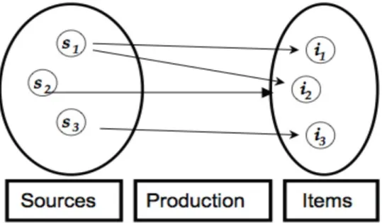
Figure 1: Information Production Process Diagram
Many of the phenomena studied in informetrics regarding the production and use of information can be represented by a triple process: the sources, the production and the items (see figure 1). This is known as the Information Production Process (IPP) (Egghe, 1990). It consists in having a set of sources and a set of items. S denotes the total number of sources and I, the total number of items. A production function quantifies the production of the items by the sources.. For an IPP, the number of sources S and the number of items I are calculated with the typical formulas:
! = !!! ! !" ! = !!! ! !"! (3)
Where f is the IPP’s size-‐frequency function and N is the maximal item per source density (in the discrete case, N designates the maximum number of items produced by a source). We use ! to represent the average number of items produced by a source:
! =!! (4)
If we consider that S and I are known ! > ! > 0 and that f is a known theoretical model, then creating a mathematical source-‐item adjustment consists in finding a necessary and sufficient condition for f to fulfil the condition (3). The term ‘mathematical adjustment’ used here designates a method introduced by Egghe within the field of informetrics to characterize inverse power distributions. It carries a different meaning from the adjustment method that is commonly used in statistics, as we mentioned in our introduction This problem was solved within the framework of Lotkaian informetrics (Egghe, 2004).
We can review the obtained results by distinguishing one case – where N, the maximum item per source density, is infinite – from the more realistic case that interests us – where N is finite, for both distributions (1) and (2).
(i) Exponential Distributions (Lafouge, 2007)
(a) N is infinite
! =!!!! (5)
! =!!!!! (6)
α depends only on the ratio !, unlike C which depends on S and µ. (b) N is finite
The adjustment conditions (3) are met by (2), ! > 1, if and only if:
! <!!!! (7)
We therefore construct f by first calculating ! ≠ 1, obtained by solving a numerical equation with one unknown.
! !! −
!"# !! !!! !!!!.! !!!!
!!!"# (!! !!! ) (8)
Where α is the parameter that verifies the inequality (7), with:
! =!!!"# (!!. !!! )!.! (9)
We can find equations (5) and (6) by making N tend toward ∞ in (8) and (9).
(ii) Inverse Power distributions (Egghe, 2004)
(a) N is infinite
When ! ≤ 2 I doesn’t exist.
If α is greater than 2, then the adjustment conditions (3) are met if and only if:
! = 1 +!!!! = 2 +!!!! (10)
! =!!!!.! (11)
α depends only on the ratio !, unlike C which depends on S and !
The value 2 of ! plays a pivotal role since the moment of order 1 can’t exist if ! ≤ 2.
(b) N is finite Two cases exist:
-‐ N ≥ 1 always exists when α ≤ 2, thus (1) meets condition (3). -‐ if α ˃ 2, the previous conclusion is valid if and only if: 2 < ! < 1 + !
!!! = 2 +
!
!!! (12)
We then construct f by calculating N, which is obtained by solving a numerical equation with one unknown. Two cases are possible:
1. ! ≠ 2 !!! ! !(!!!) !!!!− !!!!+ 1 − !!! ! !!!! = 0 (13)
Where α is a parameter verifying condition (12) with: ! =!!.(!!!)!!!!!
2. ! = 2
!" ! +!.!! −!!= 0 (14)
Where α is a parameter verifying condition (12) with: ! =!" (!)! (iii) Discussion
The calculation of α, when N is infinite – as seen in formulas (5) and (10) – is obtained through an adjustment done with the famous method of moments. This method can be used for an adjustment with an exponential distribution, but it is not suitable for an adjustment with an inverse power distribution, since the latter doesn’t always have a moment of order 1.
The most interesting case is when N is finite. It should be noted that equations (8) and (13) – where N is the unknown and α is the parameter – depend only on the average number of items produced by a source. In the Inverse power distribution case, when N is finite or infinite, the α = 2 case is a breaking point.
In these two examples, an existence theorem is used to solve the finite case – see section II.3.1.1, “the Theorem of Existence for the Size-‐frequency Function” in (Egghe, 2005).
This paper aims to provide additional elements to add to this important result. We will then recall the previous approach: the mathematical exponential (or power) adjustment of an IPP.
3. The Exponential Informetric Process and the Effort Amount
3.1 General Definition of an EIP
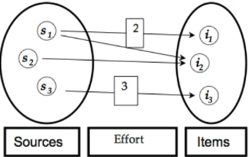
In this section, we assume that N (maximal item per source density) is infinite. We henceforth assume that each produced item requires a certain amount of effort. The difference between the IPP diagram (see figure 1) and the EIP diagram (see figure 2) is shown through the valuation of the arcs -‐ for example, in order for item i3 to be produced, source s3 must have an effort quantified by value 3.
The amount of effort needed to produce a source is generally unknown and difficult to quantify. We therefore introduce the effort function h, where h(i) is designated as the average amount of effort from a source needed to produce i items, with i= 1, 2, …. (Lafouge and Prime-‐Claverie, 2005). As previously, we work in continuous mode and define an exponential informetric process where F denotes the average quantity of effort supplied by sources to produce all the items. This paper develops the theory by using the size-‐frequency function !!!! where α is a positive number and h is
an effort function. More precisely, we have a set of functions called EF:
Figure 2: Diagram of an Information Production Process with an effort function: the EIP.
ℎ ∈ !" is called an admissible effort function if ! exists as a real positive number verifying the condition:
exp −!. ℎ ! . ℎ ! !" < ∞
!
!
We can recall results obtained in previous studies (Agouzal and Lafouge, 2008): with h being an admissible effort function, there exists a real !(ℎ) ≥ 0, so that:
∀ ! > ! ℎ !!exp −!. ℎ ! . ℎ ! !" < ∞
We thus call the size frequency function f an ‘exponential informetric process’:
! ! = !. exp −!. ℎ ! ! ∈ 1, ∞ , ! ∈ ℝ!, ℎ ∈ !", ! > ! ℎ (15)
The corresponding probability density function v is:
! ! =!.!"# (!!.! ! )! , ! ∈ 1, ∞ (16)
S is the number of sources:
! = !!!. exp −!. ℎ ! !"
And F is the average amount of effort produced by the exponential informetric process:
! = !!!. exp −!. ℎ ! . ℎ(!) !" (17)
The amount of effort F is necessarily finite, since ! > !(ℎ). It is entirely determined by the density function !, which governs the process.
The amount of produced items is written as:
The amount of items is not necessarily finite. There can therefore be an infinite amount of items produced by a finite amount of effort.
In the mathematical theory of information, the amount of effort and entropy are linked (Weaver and Shannon, 1975). When we calculate the ! ! entropy of the v process, we can prove that:
! ! = −!" ! ! + ! ! ! (19)
An exponential informetric process therefore has a finite entropy. We would have been able to define an admissible function with entropy.
m is defined as the average amount of effort produced by a source:
! =!! (20)
The average number of items produced by a source, when this number exists, is characteristic of an
IPP. Similarly, the amount of effort needed to produce a source is characteristic of an EIP. Unlike for IPPs, this average exists, for EIPs, as soon as α is higher than 1, the latter being always verified for
inverse power distributions.
3.2 Examples
3.2.1 Exponential Case
In this case, according to equation (2), the effort function is ℎ ! = ! − 1, ! ℎ = 0 and the amount of effort is:
! = ! − ! (21)
This formula is valid whether N is finite or infinite.
3.2.2: Inverse Power Case
In this case, according to equation (1), the effort function is ℎ ! = !" ! , ! ℎ = 1. We now assume that ! > 1 The amount of effort is:
1. When N is infinite:
So, following the integration: ! = !!!. exp (−!.Ln(!))!" = ! !!! ! !"(! !!! ! ! ). !"(!)!" (22) But, according to equation (16):
! =(!!!)! ! (23)
! = !. (! − 1) (24)
The amount of effort is therefore:
Hence the result:
! = 1 +!!= 1 +!! (26)
The pivotal role of 2 as a value of α is shown through the following implications:
-‐ ! < 2 implies that the amount of effort needed to produce all the items is higher than the number
of sources,
-‐ ! = 2 implies that the amount of effort needed to produce all items is equal to the number of sources,
-‐ ! > 2 implies that the amount of effort needed to produce all items is lower than the number of sources.
According to (24) and (25), entropy (19) is written as:
! ! = − ln ! − 1 + !
!!! (27)
We find the Lotka function’s (Yablonsky, 1981) expected result – the decrease of entropy, according to α.
When α ≥ 2, according to (10), the amount of effort (25) is:
! =!!. (! − !) (28)
The amount of effort is calculated according to I and S in the same way as for the exponential case. In this case, we have:
! < ! − !
The amount of effort needed during the production of an EIP that is governed by an inverse power (with α ˃ 2) is therefore smaller than an EIP governed by an exponential. This characteristic fits with the properties of informetric inverse powers distributions, as in: the more items a source has, the higher the probability that it will produce a new item.
2. N is finite
Equation (22) is written as: ! = ! !!!. !" ! . ! !!!+ ! !!! (29)
Application: calculating the amount of effort needed to produce words in a text.
To illustrate this notion, we use the typical case of a text’s word production, well known in informetrics as Zipf’s law. In this case, the number of S sources corresponds to the size of the lexicon. The total number of words in the text is the number of produced items, known as I. In (29), N designates the maximal frequency of a word in a text and is generally very high (often consisting of grammatical words such as “the” in the English language). Furthermore, we know that the distribution (frequency rank) of words in a text obeys Zipf’s law:
! ! =!!! ! ∈ 1, ! , ! > 0, ! ∈ ℝ!
! =!!!!
if N tends towards infinity and If it obeys the Zipf law, then, according to (29), the amount of effort needed to produce a text is:
! ≈ !. !
In the ideal case where β =1, the amount of effort is equal to the number of sources, i.e., to the size of the lexicon. β is generally slightly higher than 1; the effort needed to produce a text is therefore generally slightly higher than the lexicon’s size.
As to avoid any possible confusion, we must clarify certain points linked to the effort function when discussing this application to the production of words in a text.
Discussion on the Effort Function
The effort function supposes that each used (or produced) item has a certain “cost”. In his statistic theory of language (Mandelbrot, 1953), Mandelbrot introduced a cost function. Although he doesn’t mention effort functions directly, the intention remains the same:
ℎ ! = !" (!)
!" (!) (a) where V is the amount of different characters in the text and r is the word’s rank
(words are ranked by decreasing frequency). This function is based on the following hypothesis: the longer a word is, the higher the cost to produce it is.
This effort function has the following characteristics:
-‐ As the number of different characters is reduced, the number of characters in words increases, and, according to (a), the amount of effort needed to produce them increases.
-‐ The higher the rank is, the more words tend to have a large amount of characters and the rarer they are. According to (a), more effort amount is needed to produce them as the rank increases. Knowing the entropy ! and the amount of effort !, Mandelbrot then calculated the probability !(!) of a word by minimizing the average cost of information, ! =!! (see for example the proof in (Mitzenmacher 2003)).
In this case, the effort function depends on the ranking of the frequency of words and it
contributes to prove Zipf’s law. An inefficient solution would have been to say that the cost of
producing a word was proportional to the logarithm of a word’s length.
An effort function partly defines an EIP . The result in section 4 legitimizes this introduction.
4. The Necessary and Sufficient Condition for the Existence of an Exponential Informetric
Process
The exponential informetric process is defined by 4 parameters: -‐ ! > 0 as the number of sources,
-‐ ! > 0 as the amount of effort needed to produce the process, -‐ h as the effort function that characterizes the process,
-‐ ! > 1, as the maximum item per source density.
We are looking for a necessary and sufficient condition, so that C ˃ 0 and ! > 0 can exist as:
! = !!!. exp −!. ℎ ! !" ! = !!!. exp −!. ℎ ! . ℎ(!)!" (30)
Equations (30) play the same role as equations (3) in section 2. This is why we can talk about a generalisation.
Unlike section 2, N is a parameter that is supposedly known and that characterizes the process. It measures what is often referred to as the long tail of inverse power distributions. Here, the amount of effort F is what’s supposedly known, whereas the number of produced items, I, is not. At first glance, the posed problem seems unrealistic since F, unlike I, is not observable. However, studying the existence of an EIP remains interesting since it allows us to add to the previous results and to develop the notion of the amount of effort needed to produce a process, itself governed by an exponential or power-‐law distribution.
Comment
Since the effort function h is a strictly increasing positive function, with ! > 0, this implies that !. exp (−ℎ ! ) is a decreasing distribution. At first, we do not need to consider h as being admissible.
1. N is finite
With m to solve problem, (30) equates to finding a necessary and sufficient condition where ! > 0 exist and solves the following equation:
! = !"# !!.! ! .! ! !" ! ! !"# !!.! ! !" ! ! (31)
Equations (30) are indeed equivalent to: exp −!. ℎ ! . ℎ ! !" ! ! ! = exp (−!. ℎ ! !" ! ! ! = 1 !
Let N>1, for ! > 0 we define function !! as:
!! ! = !! ℎ ! − ! . exp −!. ℎ ! − ! !" (32)
Solving equation (31) means finding α ˃ 0 so that EN(α)= 0:
!! ! = 0 ⇔ ℎ ! − ! . exp (−! ℎ ! !" = 0 ! ! ⇔ ! = exp −!. ℎ ! ℎ ! !" ! ! exp −!. ℎ ! !" ! !
To conclude, α is the solution of equation (33), which depends on N, h and ! =!! :
!! ! = 0 ⇔ !! ℎ ! − ! . exp (−!. ℎ ! !" − ! !!exp −!. ℎ ! !" = 0 (33)
Lemma 4.1 We have the following results : h(1) ˂ m ˂ h (N) and EN strictly decreases.
Proof
The Equality of (31) and the fact that h strictly increases allows us to write: exp (−!. ℎ ! ℎ 1 !" ! ! exp −!. ℎ ! !" ! ! < exp (−!. ℎ ! ℎ ! !" ! ! exp −!. ℎ ! !" ! ! < exp (−!. ℎ ! ℎ ! !" ! ! exp −!. ℎ ! !" ! !
Thus, when simplifying:
ℎ 1 < ! < ℎ(!)
The calculation of the derivative is: !!! !" = − ℎ ! − ! ! ! ! . exp −!. ℎ ! − ! !"
therefore, the EN function is strictly decreasing.
This result highlights the fact that the average amount of effort needed to produce a source falls between the effort function’s minimum and maximum. We shall now demonstrate the main result of this article. For the adjustment problem (30) to have a solution – i.e. ! existing as the unique solution to the equation EN(α) = 0 – we must give a necessary and sufficient condition, linking the effort
function h, the average effort amount m and the maximal item per source density, N.
Theorem 4.1 For any N ˃ 1, then there exists α ˃ 0 as unique solution so as to have EN (α) = 0, if and
only if: ! =! !∈ ℎ 1 , ℎ ! !" ! ! ! − 1 Proof
(i) Necessary Condition
According to the 4.2 lemma, EN is a strictly decreasing function, so ! > 0 implies that:
0 = !! ! < !! 0 = !! ℎ ! − ! !" Then: ℎ 1 < ! < ℎ ! !" ! ! ! − 1
(ii) Sufficient Condition
The inequality of the 4.1 lemma and the intermediate value theorem implies that there exist ! ∈ 1, ! (unique solution, since h is strictly increasing) so that m = h(y); when u ˂
y, then ℎ ! − ! < 0 and ! − ! > 0 when u ˃ y, then:
!! ! = !! ℎ ! − ! . exp (−!. ℎ ! − ! !" + !! ℎ ! − ! . exp (−!. ℎ ! − ! !"
Since EN is strictly decreasing and !! 0 = !! ℎ ! − ! > 0 we can therefore conclude
that ! > 0, with EN (α) = 0 as the unique solution
2. N is infinite
Although we aren’t covering this case as a whole, two comments can be made.
First, when N is infinite, we must assume that the effort function h is admissible for F and m to be finite. An important property then completes the theorem.
Lemma 4.2 If N tends towards infinity, then the function ! ! = ! ! !"
! !
!!! tends towards infinity and
is an increasing function.
Proof
Since h isn’t bounded, ∀ ! > 0 N so that ∀! > !, ℎ ! > ! then !!ℎ ! !" > ! − 1 ! therefore ! ! !" ! ! !!! > !
therefore g is not bounded.
The calculation of the derivative !"(!) !" = ℎ ! . ! − 1 − !!ℎ ! !" (! − 1)!
is positive, therefore g is increasing.
Discussion Before working on examples, we must think about the significance of such a result. First of all, we notice that, in the same way as for an IPP, the normalizing factor C doesn’t play a part in this problem. It is entirely determined by α.
Lemma 4.2 allows us to precise the results of theorem 4.1. Supposing that we are in a stable process in which the number of sources is mostly fixed, the amount of effort increases slightly. Let’s suppose that the necessary condition for the existence of an EIP is verified. Then, if N – the maximum number of items a source can produce – increases over time, then the condition of existence is always verified.
Let’s take, as an example, the case where a relatively long text is produced. Let’s suppose that the text is lengthened over time by its author. We can suppose that the size of the lexicon doesn’t change very much. If the amount of effort increases slightly, the condition of theorem 4.1 remains true because of the fact that a word’s maximal frequency, generally a grammatical word, becomes very high.
5. Examples of Processes
This theorem is now applied to the two types of distributions seen above in the context of IPPs.
5.1 Exponential Process
We shall call this method as follows: the mathematical exponential adjustment of an EIP.
1. N is finite
! = ! − ! and the effort function is ℎ ! = ! − 1. According to theorem 4.1, for any ! > 1, and
! =!!∈ 0,!!!! (34)
α exists as unique solution to (33) :
!!!. exp (−!. ! − 1 !" − (1 + !) !!exp −!. ! − 1 !" = 0
According to (21), we have ! + 1 =!!
Following calculations, we then find, the same equation (8) as for the mathematical exponential adjustment of an IPP. Hence (30) implies that:
! =!!!"# (! !!! .!)!.!
Remarks
Equations for IPPs and EIPs are identical, but the solved problems are different. If we call this equation Fe, it depends on three values, α, m and N, which all play different roles in each equation. If we call the unknown x, then:
-‐ In the case of an IPP, we find a necessary and sufficient condition for the equation Fe (x, α, m) = 0 (here, x = N) to have a unique solution:
! < 1 !
-‐ In the case of an EIP, we find a necessary and sufficient condition for the equation Fe(N, x, m) = 0 (here x= α) to have a unique solution :
! <! − 1 2
We therefore proved the following result. Where ! > 1, ! > ! > 0, a necessary and sufficient condition for ! > 0 and ! > 0 to exist, verifying :
! = !!!. exp !. ! − 1 !" ! = !!!. exp !. ! − 1 (! − 1) !" (36) is ! < ! !!! !!! ! < !!! ! (37)
We can illustrate this result with a numerical example.
2. Numerical example N°1
-‐ The mathematical exponential adjustment of an EIP
Let S = 5,000 F= 15,000 and N= 10 , then I = 20,000 and m= 3, we have equation (8) that takes the form of (38) (replacing α by x):
4! −!"# (!!!))(!!!!"!)!!!!!!!"# (!!!) (38)
Which can be solved (since (34) is true) by using the MAPPLE 17 software, for e.g. we find x≈ 0.239=α (35) implies that C ≈ 1, 352. To conclude, the exponential distribution is:
! ! ≈ 1,352. exp −0.239. ! − 1 ! ∈ 1,10 (39)
The result is coherent since the condition (7) of the mathematical exponential adjustment of an IPP is verified:
0.239 = ! <!!!! =!! = 0.33
-‐ The mathematical exponential adjustment of an IPP
We use the same values as the previous example.
Let S= 5,000, I= 20,000 and α = 0.239 then equation (8) takes the form of (40) (replacing N by x):
0.956 − !"# !!.!"#!!!.!"# !!.!"#!!! !!.!"#
!!!"# !!.!"#!!!.!"# = 0 (40)
Which can be solved (since (7) is true) by using the MAPPLE 17 software, for e.g. we find the expected result, which is x≈ 10 = N.
The result is coherent since the condition (34) of the mathematical exponential adjustment of an EIP is verified:
! =!!!! = 3 <!!!! = 4.5
3. N is infinite
If N tends towards infinity, then the equation is written as:
!!. ! − ! − 1 = 0
With the value of α being: ! =!! =! != ! !!! (41)
We also have: ! =!!!!!
We obtain the same result (see 5 and 6) as for the mathematical exponential adjustment of an IPP. This result was expected since the effort function in the exponential model is the identity function. The mathematical exponential adjustment of an IPP and the mathematical exponential adjustment of an EIP are identical.
Discussion Conditions (37) for the existence of an IPP that is governed by an exponential process are complete. For the exponential case, the amount of effort does not need to be known. All that needs to be known are the 3 essential characteristics of a distribution. The inverse power case is very different, as we are about to see.
5.2 Inverse Power Process
We shall call this method as follows: the mathematical inverse power adjustment of an EIP.
1. N is finite
The effort function is log u. According to theorem 4.1, for any N˃1, and
! =!!∈ 0,!.!" ! !!!!!!! (42)
There exists α, solution of (33):
ln (!) !! ! ! !" − ! 1 !! ! ! !" = 0
Therefore the equation to be solved is: !!!! !! ! !!"!!! . ln ! !" − !. !!!! ! !" = 0 Following calculations: ! !!!Ln N . ! !!!+ 1 − !!!! ! !!!+ ! !!!! = 0 (43)
We also have, according to (30), the normalizing coefficient:
! = !.(!!!)
!!!!!! (44)
2. Numerical example N°2
Let S =10,000, F=6,000 and N = 10; we have and ! =!! and:
!.!" ! !!!!!!! = 1.5584
Equation (43) takes the following form (replacing α by x): !" !" .!"!!! !!! + 1 − 10!!! . ( !.! !!!+ ! (!!!)!) = 0 (45)
Since condition (42) is verified, this equation can be solved by using the MAPPLE 17 software, for e.g. we find x ≈ 2.47 = α. (44) implies that C ≈ 15,215. To conclude, the power distribution is:
! ! ≈ 15,215.!!.!"! ! ∈ 1,10 (46)
Let S=5,000, F=7,000 and N=50 we have m=1.4
!. !" ! − ! + 1
! − 1 = 2.991
Equation (43) takes the following form (replacing α with x): !" !" .!"!!! !!! − 1 − 50!!! . !.! !!!+ ! !!!! = 0 (47)
Since condition (42) is verified, this equation can be solved by using the MAPPLE 17 software, for e.g. we find x ≈ 1.46 = α. (44) implies that C ≈2,679. To conclude, the power distribution is:
! ! ≈!,!"#!!.!" ! ∈ 1,50 (48)
4. N is infinite
If N tends towards infinity, then (43) is written as follows: ! 1 − !+ 1 (1 − !)!= 0
With the value of α being: ! = 1 + ! != 1 + ! ! (49)
We find the expected result (see (26)) for the value of α. Furthermore, we deduce, based on (30), that:
! = !. (! − 1)
If α ˃ 2, then, according to (28), the equation (49) is written as follows: ! = 1 + ! ! − ! and ! = !. ! ! − !
i.e., the same result (see (10) and (11)) as for a mathematical inverse power distribution adjustment.
Discussion
In the case where N is infinite, we demonstrated the formula ! = 1 +!! . This formula is
true, whatever α’s value. The more the effort amount F decreases (or, the more entropy decreases), the more α increases. This means that the gap widens between a large number of sources that produce little and a small number of sources that produce a lot. Unlike in the case of an (IPP), the value α =2 is not a breaking point.
In the two numerical examples that were considered, when we compare the value of α, solution to the equation, it is roughly equal to 1 +!!
Example 2: exact calculation of α , 2.47, rough formula α ≈ 2.67 Example 3: exact calculation of α , 1.46, rough formula α ≈ 1.7
We can compare the necessary and sufficient conditions for the existence of an exponential process and of an inverse power process. For N ˃ 1, the inequality is as follows:
!.!" ! !!!!!!! ≤ !!!
!
This inequality implies that if the mathematical power adjustment of an EIP is verified, then the same applies for a mathematical exponential adjustment. This result concurs with the mathematical adjustment of an IPP (see theorem 5 (Lafouge, 2007)).
If N is infinite, it is worth making a parallel between the coefficient α of the exponential (41) and of the inverse power (49).
! =!! ! = 1 +!!
This analogy allows us to better understand the role that the amount of effort plays in exponential and inverse power distributions.
Before concluding, it is important to clarify certain points – as we did for the effort function – so as to get more insight into the contributions and limits of this research.
Discussion: Limits and Contributions
The numerical examples used in this article weren’t drawn from real situations. It is currently difficult for us to present such real results. The crucial problem lies in knowing the amount of effort – which is unknown and tied to the effort function, itself also unknown, as was shown above. We would need to perform calculations in a real life setting and choose a realistic value for F. We could then compare it with results obtained using the classic Lotkaian case.
The main contribution in creating an EIP lies in the fact that the EIP highlights the connection – though already known – between the amount of effort (or entropy (see (19)) as understood by Shannon) and informetric distributions. Lotkaian distributions serve to explain many statistical regularities. It therefore seems important to draw attention to two points:
-‐ the role of the logarithm effort function. In a previous article (lafouge T and Smolczewska 2006), we showed that, if h is an effort function – positive, strictly increasing and unbounded – that verifies the relation
lim
!→!
ℎ(!)
ln (!)= ! ! > 1
then h is admissible and the amount of effort is finite. Unfortunately, such a condition is not necessary.
-‐ We also want to highlight the pivotal point of ! = 2, since it corresponds to the case where the amount of effort is equal to the number of sources.
6. Conclusion
Both models are compared: the mathematical adjustment of an IPP initiated by Egghe, and the mathematical adjustment of an EIP, presented in this article. This is relevant only if the distribution is of the power or exponential type.
When N is infinite, the mathematical exponential adjustments of an IPP and of an EIP is identical. When N is infinite and α ˃ 2, the mathematical power adjustment of an IPP and of an EIP are identical.
Results differ in a realistic case, when N is finite. In the exponential case, the mathematical
adjustment of an EIP completes the result previously found for an IPP. This is due to the fact that the effort function is the identity, therefore ! = ! − ! whatever the value of N. In the power case, the value α = 2 is not a breaking point for an EIP, whereas it is for an IPP. It would be interesting to study other effort functions (Lafouge and Smolczewska, 2006) in order to expand on the notion of EIP adjustments.
References
Agouzal, A. and Lafouge, T. (2008). On the relation between the maximum entropy principle and the principle of least effort : The continuous case. Journal of Informetrics, 2 :75–88.
Albaran, P. and Castillo, C. (2011). References made and ci-‐tations received by scientific articles.
Journal of the American Society for Information Science and Technology, 62 :40–49.
Clauset, A., Slalizi, C., and Newman, M. (2009). Power-‐law distribution empirical data. SIAM Reviews, 51 :661–771.
Egghe, L. (1990). On the duality of informetric systems with application to the empirical law. Journal
of Information Science, 16 :17–27.
Egghe, L. (2004). The source-‐item coverage of the lotka function. In Scientometrics, 59(2) :225–232.
Egghe,L.(2005). Power Laws in the Information Production Process: Lotkaian Informetrics. Elsevier.
Lafouge, T. (2007). The source-‐item coverage of the exponential function. Journal of Informetrics, 1 :59–67.
Lafouge, T. and Prime-‐Claverie, C. (2005). Links between entropy and production of information, characterization of informetric distribution ising the effort function, exponential informetric process.
Information Processing and Management, 41 :1387–1394.
Lafouge, T. and Smolczewska, A. (2006). An interpretation of the effort function trough the mathematical formalism of exponential informetric process. Information Processing and
Management, 42 :1442–1450.
Mandelbrot, B. (1977). The Fractal Geometry of nature. Freeman, New York USA
Mitzenmacher, M. (2003). A brief history of generative models for power law and lognormal distribution. Internet Mathematics, 1(2) :226-‐251
Petruszewycz, M. (1972). Loi de pareto ou loi log-‐normale : un choix difficile. Mathématiques et
sciences humaines, 39 :37–52.
Weaver, W. and Shannon, C. E. (1975). Théorie mathématique de la communication. La bibliothèque du CEPL.
Yablonsky, A. (1981). On fundamental regularities of the distribution of scientific productivity.
Scientometrics, 2(1) :3–34.