HAL Id: inria-00436753
https://hal.inria.fr/inria-00436753
Submitted on 27 Nov 2009
HAL is a multi-disciplinary open access
archive for the deposit and dissemination of
sci-entific research documents, whether they are
pub-lished or not. The documents may come from
teaching and research institutions in France or
abroad, or from public or private research centers.
L’archive ouverte pluridisciplinaire HAL, est
destinée au dépôt et à la diffusion de documents
scientifiques de niveau recherche, publiés ou non,
émanant des établissements d’enseignement et de
recherche français ou étrangers, des laboratoires
publics ou privés.
Nicolas Mansard, François Chaumette
To cite this version:
Nicolas Mansard, François Chaumette. Directional redundancy for robot control. IEEE Transactions
on Automatic Control, Institute of Electrical and Electronics Engineers, 2009, 54 (6), pp.1179-1192.
�inria-00436753�
Directional Redundancy for Robot Control
Nicolas Mansard and François Chaumette, Member, IEEE
Abstract—The paper presents a new approach to design a con-trol law that realizes a main task with a robotic system and simulta-neously takes supplementary constraints into account. Classically, this is done by using the redundancy formalism. If the main task does not constrain all the motions of the robot, a secondary task can be achieved by using only the remaining degrees of freedom (DOF). We propose a new general method that frees up some of the DOF constrained by the main task in addition of the remaining DOF. The general idea is to enable the motions produced by the secondary control law that help the main task to be completed faster. The main advantage is to enhance the performance of the secondary task by enlarging the number of available DOF. In a formal framework, a projection operator is built which ensures that the secondary control law does not delay the completion of the main task. A control law can then be easily computed from the two tasks considered. Experiments that implement and vali-date this approach are presented. The visual servoing framework is used to position a six-DOF robot while simultaneously avoiding occlusions and joint limits.
Index Terms—Gradient projection method, redundancy, robot control, sensor-feedback control, visual servoing.
I. INTRODUCTION
C
LASSICAL control laws in robotics are based on the min-imization of a task function which corresponds to the re-alization of a given objective. Usually, this main task only con-cerns the position of the robot with respect to a target and does not take into account the environment where the robot evolves. However, to integrate the servo into a real robotic system, the control law should also make sure that it takes into account any necessary constraints such as avoiding undesirable configura-tions (joint limits, kinematic singularities, or sensor occlusions). Two very different approaches have been proposed in the lit-erature to deal with this problem. A first solution is to take into account the whole environment from the very beginning into a single minimization process, for example by pre-computing a trajectory to be followed to the desired position [18] or by de-signing a specific global navigation function [6]. This provides a complete solution, which ensures the obstacles avoidance when moving to complete the main task. However, the pre-computa-tions (construction of the trajectory or of the navigation func-tion) require a lot of knowledge about the environment, and inManuscript received December 21, 2005; revised February 20, 2007. First published May 27, 2009; current version published June 10, 2009. This paper was presented in part at the IEEE 44th IEEE Conference on Decision and Control and European Control Conference (ECC-CDC’05), Sevilla, Spain, December, 2005. Recommended by Associate Editor J. P. Hespanha.
N. Mansard was with INRIA Rennes-Bretagne Atlantique-IRISA, Rennes 35042, France and is now with LAAS, CNRS, Toulouse 31077, France (e-mail: [email protected]).
F. Chaumette is with INRIA Rennes-Bretagne Atlantique-IRISA, Rennes 35042, France (e-mail: [email protected]).
Color versions of one or more of the figures in this paper are available online at http://ieeexplore.ieee.org.
Digital Object Identifier 10.1109/TAC.2009.2019790
particular about the constraints to take into account. This solu-tion is thus less reactive to changes in the goal, in the environ-ment or in the constraints.
Rather than taking into account the whole environment from the very beginning, another approach considers the secondary constraints through an objective function to be locally mini-mized. This provides very reactive solutions, since it is very easy to modify the objective function during the servo. A first solution to take the secondary objective function into account is to realize a trade off between the main task and the constraints [19]. In this approach, the control law generates motions that try to make the main task function decrease and simultaneously take the robot away from the kinematic singularities and the joint limits. On the opposite, a second solution is to dampen any motion that does not respect the constraints. This solution has been applied using the weighted least norm solution to avoid joint limits [3]. The control law does not induce any motion to take the robot away from the obstacles, but it forbids any motion in their direction. Thus, it avoids oscillations and unnecessary motions.
However, these two methods can strongly disturb the execu-tion of the main task. A second specificaexecu-tion is thus generally added: the secondary constraints should not disturb the main task. The Gradient Projection Method (GPM) has been initially introduced for non-linear optimization [20] and applied then in robotics [7], [10], [15], [21]. The constraints are embedded into a cost function [13]. The gradient of this cost function is com-puted as a secondary task that moves the robot aside the obsta-cles. This gradient is then projected onto the set of motions that keep the main task invariant and added to the first part of the con-trol law that performs the main task. The main advantage of this method with respect to [19] and [3] is that, thanks to the choice of the adequate projection operator, the secondary constraints have no effect on the main task. The redundancy formalism has been used in numerous works to manage secondary constraints, for example force distribution for the legs of a walking ma-chine [14], occlusion and joint-limit avoidance [17], multiple hierarchical motions of virtual humanoids [1], or human-mo-tion filtering under constraints imposed by the patient anatomy for human-machine cooperation using vision-based control [9]. However, since the secondary task is performed under the con-straint that the main task is realized, the avoidance contribution can be so disturbed that it becomes inefficient. In fact, only the degrees of freedom (DOF) not controlled by the main task can be exploited to perform the avoidance. The more complicate the main task is, the more DOF it uses, and the more difficult to apply the secondary constraints. Of course, if the main task uses all the DOF of the robot, no secondary constraint can be taken into account.
Nevertheless, even if a DOF is controlled by the primary con-trol law, the constraints should be taken into account if it “goes
in the same way” as the main task. Imposing the control law part due to the constraints to let the main task invariant can be a too strong condition. We rather propose in this article a more general solution that only imposes to the secondary control law not to increase the error of the main task (to preserve the sta-bility of the system), that is when the secondary task goes in the same direction than the main task. This method is thus called
directional redundancy. By this way, the free space on which
the gradient is projected is larger. More DOF are thus available for any secondary constraint, and the control law derived from the applied constraints is less disturbed.
The paper is organized as follow. In Section II, we recall the classical redundancy formalism and build using the same continuous approach a new projection operator that enlarges the projection domain. We then propose in Section III to use a sampled approach to compute a similar projection operator, in order to improve the global behavior of the system. If the control law due to the main task is stable, which is the usual hy-pothesis, the obtained control law is proved to be stable, and to asymptotically converge to the completion of the main task and to the best local minimum of the secondary task (Section IV). For the experiments, the proposed method has been applied to a visual servoing problem. Visual servoing consists in a closed loop reacting to image data [4], [7], [8], [11], [12]. It is a typical problem where the constraints of the workspace are not con-sidered into the main task. The visual servoing framework is quickly presented in Section V. Finally, Section VI describes several experiments that show the advantages of the proposed method.
II. DIRECTIONAL REDUNDANCY USING ACONTINUOUSAPPROACH
In this section, the classical redundancy formalism is first re-called. Based on this formulation, we deduce a more general way to take the secondary term into account, by enlarging the free space of the main task. The stability of this new control law is then proved. We conclude by explaining the limitations of this control scheme. To solve these limitations, a second-order derivation is necessary, as done in Section III.
A. Considering Only the Main Task
Let be the joint position of the robot. The main task function is . It is based on features extracted from the sensor output. The robot is controlled using the joint velocities . The Jacobian of the main task is defined by
(1)
Let be the number of DOF of the robot and be the size of the main task . The task function is designed to be full rank, i.e. [21].
The task function is the controller input, and the robot joint velocity is the controller output. The controller has to regu-late the input to according to a decreasing behavior chosen
when designing the control law. By inverting (1), the joint mo-tion that realizes this required decrease of the error is given by the least-square inverse
(2) where the notation refers to the Moore-Penrose inverse of the matrix [2]. By (2), we consider that the Jacobian matrix is perfectly known. If it is not the case, due to inaccuracy in the calibration process or uncertainties in the robot-scene model, an approximation has to be used instead of . It is possible to prove that (2) is stable [21]. In the following, we make the assumption that is perfectly known, from which we deduce . We also assume that is a stable vector field, that is to say it is possible to find a correct Lyapunov func-tion so that if , then and (2) is asymptotically stable.
It is classical to specify the control scheme by an exponen-tial decoupled decreasing of the error function, by imposing , where is a positive parameter that tunes the con-vergence speed. This finally produces the classical control law . In that case, a classical Lyapunov function is based on the norm , e.g. .
B. Classical Redundancy Formalism
The solution (2) computed above is only one particular so-lution of (1): it is the soso-lution of least norm that realizes the reference motion
(3) The redundancy formalism [21] uses a more general solution which enables to consider a secondary criterion. The robot mo-tion is given by
(4) where is the projection operator onto the null space of the matrix (i.e., ), and is an arbitrary vector, used to apply a secondary control law. Thanks to , this secondary motion is performed without disturbing the main task having priority.
It is easy to check that the joint motion given by (4) pro-duces exactly the specified motion in the task function space (5)
since and . The joint
motion is chosen to realize exactly the motion in the task function space, and to perform at best a secondary task whose corresponding joint motion is . Looking at (3), the motion obtained in (4) is simply another solution of (1), however not minimal in norm.
It is easy to check that the addition of the secondary term does not modify the stability of the control law. Let be a Lyapunov function associated to control law (2) (that is to say such that ). Then is also a correct
Lyapunov function for the control law (4). In fact, does not depend of the secondary term
(6)
where is the reference decrease speed, obtained when considering only the main task.
C. Extension of the Convergence Condition
In the classical redundancy formalism, the secondary control law is applied under the condition that it does not modify the convergence speed , that is to say under the condition
. However, to guarantee the convergence of the main task, it is sufficient to ensure that the convergence is at least as fast as . The condition of application of the secondary control law can thus be written
(7) In the following, we propose a solution to apply the secondary control law under Condition (7). By analogy with the classical redundancy formalism, we search a control law of the following form:
(8) We search the condition on such that this control law respects (7). When (8) is applied, can be written
(9) By introducing this last equation in (7), a simpler form of the condition is obtained
(10)
where .
D. Construction of the Extended Projection
In this section we build an operator that projects any sec-ondary control law to keep only the part respecting (10). Let be any secondary control law. We note , and we search
so that respects (10).
To simplify the formulation, adequate bases of both joint and task function spaces are chosen. Let , and be the result of the SVD of :
(11) with a basis of the joint space, a basis of the task func-tion space, , and the diagonal matrix whose coefficients are the singular values of , noted . Condition (10) can thus be written
(12) where and . To simplify the con-struction of the projection operator, this condition is restricted to the following:
(13)
where . This condition is more restrictive than the previous one. However, it ensures a better behavior of the robot. Particularly, if the Lyapunov function is the norm of the error (as classically done), this condition ensures the con-vergence of each singular components of the error separately, while (10) ensures only the convergence of the norm of the error, which can lead to a temporary increase of one or several com-ponents. This can cause some troubles during the servo. For ex-ample, in visual servoing, it can cause the loss of some features during the robot motion. By (13), we ensure that each compo-nent will be faster than the required motion , avoiding thus such problems.
Let us now consider any secondary control law . We note . To build a secondary term from that respects (13), we just have to keep the components that respects the inequality, and to nullify the others: for all
if or
if and have opposite signs if and have the same sign
(14)
This equation can be put under a matricial form
. .. (15) where the components of are defined by
if or
if and have opposite signs if and have the same sign It has to be noticed that is not linear: the associated matrix
is computed from . The term is thus not linear in . The control law that realizes the main task and ensures that the secondary control law respects Condition (13) can finally be written
(16)
where .
E. Stability of the Control Law
The computations that bring to the control law (16) prove the following result:
Theorem 2.1: Let be any task function whose Jacobian is full rank. If the following control law:
(17) is applied to the robotic system, where:
• is a stable vector field, that is to say it is possible to find an associated Lyapunov function such that if , then ;
• is any secondary control vector;
then the error asymptotically converges to zero.
F. Potential Oscillations at Task Regulation
The control law (16) is composed of two terms. The first one is linearly linked to . The second term is , whose only constraint is that each component has the proper sign. It is
Fig. 1. Comparison of the free spaces using the classical redundancy frame-work, one bound (Section II) and two bounds (Section III). If the classical re-dundancy formalism is used, the secondary control law is projected onto the null space of the main task: the secondary termsz are projected on the corre-spondingPz (i = 1 . . . 3). When only one bound is used, the free space is a “half-plane”: the blue region is forbidden. The secondary termsz and z are not modified by the projection. However, the action ofz on the main task is very important, and may result in oscillations or even instability, in particular if the time interval between two iterations is large. A second bound is then added: the green region is forbidden too. The secondary termz is then projected on P z , which prevents any oscillation at task regulation.
thus not proportional to the error to regulate, and can be arbi-trarily large when the main task converges to 0.
When applied in practice, this control law may introduce os-cillations when the main task converges, due to a too large value of . The effect is very similar to the oscillations induced by a too large value of the gain on a sampled system. To correct this problem, it is necessary to introduce an upper bound on the value of the secondary term, in order to narrow the free space to a band whose width depends on the value of the main-task error (see Fig. 1). This upper bound appears directly when condition of projection is computed from a second-order expansion of the Lyapunov function, as it will be shown in the next section.
III. DIRECTIONAL REDUNDANCY USING ADISCRETEAPPROACH
As explained in the previous paragraph, using only one bound can lead to oscillations when considering a sampled system. In this section, we present a solution to introduce a second bound. This requires to consider the robot as a discrete system.
As in the previous section, we want to ensure the convergence of the Lyapunov function at least as fast as when the main task is considered alone. The condition of application of the secondary control vector can thus be written
(18)
where and is
the desired behavior of the main task and is the sampling interval.
In the previous section, we have considered a first order ap-proximation of . Let us now consider the second-order Taylor
expansion of the Lyapunov function when the small displace-ment is applied
where denotes a term whose norm is asymptotically bounded by . Since and since and are asymptotically of the same order, this last equation can be written
(19) As previously, the control law can be searched under the fol-lowing form, without any loss of generality:
(20) where is any secondary control law. Introducing this last form in (19), we obtain
Since and using the second order decomposition (19) of , the condition (18) can be rewritten
(21) For the construction of the control law, the term is neglected and the condition of application of the secondary term
is finally reduced to
(22)
This condition can be compared to the condition (10) ob-tained in the last section. First of all, if the second-order derivative is neglected, both conditions are equiva-lent. When the second-order derivative is taken into account, (22) implies a quadratic form of the secondary control law . Intuitively, one can see that this quadratic term will lead to a lower bound and a upper bound on the value of , which is exactly what is required.
A. Rewriting the Condition
The inequality (22) is difficult to solve in the general case, since it implies a quadratic term on weighted by . To simplify the computation, we make the assumption that the second-order derivative is the identity. This is the case when considering the norm of the error as a Lyapunov function
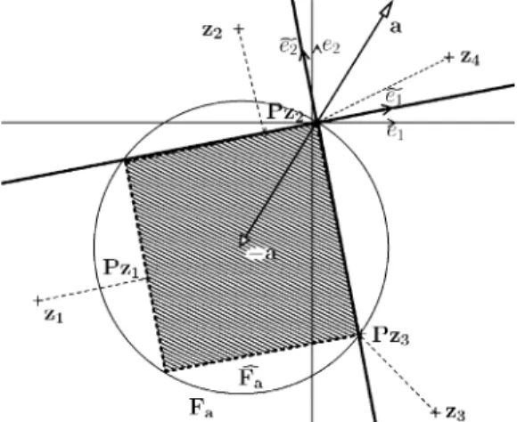
Fig. 2. Two setsF (the circle) and F (the dashed rectangle) in dimension 2. The canonical basis of the task space is(e ; e ). The SVD coordinate frame is (e ; e ). In this basis, the set F is simply a ball of euclidean norm k:k, with center0a and radius kak, and the set F is the same parameters ball of norm k:k . The four points z , z , z and z are projected into F as a matter of example. Their projection is respectivelyPz , Pz , Pz and 0. The projection is realized by applying the projection operator computed in Section III-C.
, which is a very classical solution. We thus consider the following condition:
(23)
where .
As in the previous section, the SVD bases are introduced to reduce the complexity to the case where the Jacobian is diag-onal. We note and . Condition (23) can be simply written as
(24)
By adding the term to both sides of the in-equality, the following factorization is obtained:
(25)
B. Construction of the Free Space
For some vector , let be the set
(26) is the ball of radius and center . It is represented on Fig. 2 in the case of a 2-D vector space. Using this definition, the set of all the possible secondary motions such that respects the condition (23) is characterized easily. This condi-tion can thus be written as
(27) Given an arbitrary secondary command , we now want to modify this vector to obtain a second term that respects this condition. If belongs to the free space , it can be
directly added to the primary control law . Other-wise, it has to be projected into the free space. The projection operator is computed using the analytical parametrization of . By developing the square of the norms in (25), it is easy to obtain after some simple calculations
(28)
This last condition imposes a decrease of the norm of the error. As in the previous section, we reduce the condition by imposing the decrease of each component of the error. The set is reduced to its Cartesian subset. A sufficient condition is thus
(29)
The set defined by (29) is noted . It is represented with the corresponding set on Fig. 2. is in fact the ball defined by the norm , where
(30)
C. Construction of the Projection Operator
The projection operator into the free space is noted . It is a vectorial operator that transforms any vector into a secondary control law such that (29) is respected, and such that the distance is minimal. Using the an-alytical characterization of the free space given by (29), this projection operator can be computed component by component within basis .
Since , (29) can be developed by dividing by (if is not zero): belongs to the free space of the main task if and only if
(31)
For each component of , the closest that respects (31) can be computed. By analyzing each case separately, the general expression of is deduced if or if if if and if and otherwise. (32) This equation can be written under a matricial form
Fig. 3. Comparison of the projection operators obtained with the classical redundancy formalism, and with the directional redundancy, first order (15) and second order (33). where if or if if if and if and otherwise.
As in Section II, the operator is not linear: the term is thus not linear in . Moreover, in that case, the matrix is not a projection matrix (its diagonal should be composed only of 0 and 1). It is only the matricial form of the non linear projection operator .
D. Control Law
The projection operator is computed into the SVD bases and . We note this operator into the canonical basis of the joint space
(34) The control law is finally written. Thanks to the matricial form , the obtained form is very close to the classical redundancy form given in (4)
(35) where is an arbitrary vector, used to perform a secondary task without disturbing the decreasing speed of the main task error.
E. Comparisons and Conclusion
A comparison between the two projection operators built in Sections II and III with the classical projection operator is given in Fig. 3. As in the classical formalism, the projection operator is used to transform any secondary vector into a secondary control law that does not disturb the main task. Within the same basis , the projection operator of the classical redundancy is also a diagonal matrix, but whose coefficients are
if
otherwise. (36) In other terms, the first projection operator (15) that we have de-fined has more non zero coefficients. When a component of the main task function is not zero, a DOF is freed up. Furthermore, the proposed formalism accelerates the decreasing of each com-ponent of the error and takes the secondary task into account in the same way.
Compared to the projection operator (15), the operator (33) induces an alleviation if the secondary control law is too impor-tant wrt. the error value. In particular, at task completion, when the error vector is nearly zero, this allows to reduce the effect of the secondary term, and to avoid any oscillation.
IV. STABILITY OF THECONTROLLAW
The definition of the control law (35) and the associate pro-jector lead to the following theorem:
Theorem 4.1: Let be any task function whose Jacobian is full rank. If the following control law:
(37) is applied to the robotic system, where:
• is a stable vector field such that
respects .
• is any secondary control law, and is defined by (33). then, given that is sufficiently small, the error asymptoti-cally converges to zero.
Proof: From (21), it is possible to write
(38) By construction of , we know that respects (22). Introducing (22) in the previous equation, we obtain
(39) Subtracting from both side of the inequality finally gives
(40)
where and
. It is thus possible to find small enough to have . Since has the same order as and given that is sufficiently small, then . By definition of ,
is negative, which proves that is a correct Lyapunov function for control law (37).
Remark 1: We have not been able to determine any
theoret-ical value of to ensure the stability for any large value of . In practice, the value of used to compute the control law could be chosen smaller than the actual value of the sampling interval of the control input. This choice allows ensuring the practical stability of the system when is large. However, we have not used the possibility to tune this parameter in the ex-periments presented in the following: has been chosen equal
to the system time interval. No unstability have been noticed during the experimental setup.
Remark 2: Theorem 4.1 supposes that the desired evolution
is such that is negative. When as classically done, this last hypothesis is simply obtained by choosing the gain and the step size small enough.
Theorem 4.1 only gives the asymptotic convergence of the main task. It does not say anything about the secondary task. Since the main task has priority, the convergence of the sec-ondary task can not be ensured in the general case. However, it is expected to obtain at least the convergence of the part of the secondary task located inside the null space of the main task, that is to say
(41) In the general case where the secondary task can be any -di-mensional vector, nothing can be proved. We thus limit the sta-bility study to the classical case where the secondary task is the gradient of a cost function to be minimized [13], [17]. Indeed, the secondary tasks used to experiment the control law on the robot are derived from a cost function (see Section V-B). Using Theorem 4.1, it is easy to deduce the asymptotic convergence to a region where the secondary task gradient is in the null space of the main task, that is to say the cost function is asymptotically minimized under the constraint .
Corollary 4.1: Let be any positive convex function de-fined on the joint space. Using the hypotheses of Theorem 4.1, if the control law (37) is applied to the robotic system, with , then the cost function is asymptotically mini-mized under the constraint .
Proof: The control law is asymptotically equivalent to
(from Theorem 4.1)
(42) We assume that does not depend of the independent time vari-able
(43) By introducing (42) in (43), we obtain
(44) Since is definite non-negative for any vector (due to the form (33) of the coefficients of the equivalent diagonal matrix
), we finally obtain
(45) This result is sufficient to prove the stability of the secondary criterion, but does not prove that the second criterion is globally asymptotically minimized ( should be negative, and it is only non-positive). However, it proves that is stable and decreases until becomes null, that is the minimum under the constraint is reached.
A similar Lyapunov function can be given for the control scheme using the classical redundancy formalism. Let be the secondary cost function value over time using the classical redundancy formalism scheme, and let be the secondary
cost function value using the scheme proposed in Theorem 4.1. Through the misuse of notation , we can write
(46) (47) Since the singular values of are all greater than or equal to the singular values of (due to (33) and (36)), the following inequality can be written:
(48) The cost function converges to similar local minima using both schemes. However, this last inequality proves that the conver-gence is faster using the directional redundancy.
To conclude, we have shown in this section that the global minimization of is of course not necessarily ensured. The system converges to a local minimum imposed by the constraint as expected. However Theorem 4.1 and Corollary 4.1 prove that the system is globally stable, and asymptotically con-verges to the main task completion and to the best reachable local minimum of the secondary task.
V. APPLICATION TOVISUALSERVOING
All the work presented above has been realized under the only hypothesis that the main task is a task function as described in [21]. The method is thus fully general and can be applied for numerous sensor-based closed-loop control problems. For this article, the method has been applied to visual servoing. In the experiments described in the next section, the robot has to move with respect to a visual target, and simultaneously to take into account a secondary control law. For the simulations, this secondary term was simply an arbitrary velocity. For the exper-iments on the real robot, the joint limits and possible occlusions were considered. In this section, the classical visual servoing formalism is first quickly recalled (Section V-A). Two avoid-ance laws are then presented for joint-limit and visual-occlu-sion avoidance, based on the gradient of a cost function [13], [15], [17]. We have chosen to use a solution proposed from path planning [18] which ensures an optimal computation of the gra-dient by the use of a pseudo inverse. This general method is presented in Section V-B and the two cost functions are given in Section V-C.
A. Main Task Function Using Visual Servoing
In the experiments presented below, an eye-in-hand robot has to move with respect to a visual target (a sphere in simulation and a rectangle composed of four points easily detectable for the experiments on a real robot). By choosing a very simple target, the experiments have focused on the control part of the work.
The task function used in the following is defined as the difference between the visual features computed at the current time and the visual features extracted from the desired image [7], [12]:
(49) The interaction matrix related to is defined such that
it is clear that the interaction matrix and the task Jacobian are linked by the relation
(50) where the matrix denotes the robot Jacobian and is the matrix that relates the camera instantaneous velocity to the variation of the chosen camera pose parametrization
. The classical proportional control law
was used. The control law finally used in the experiment is then (51) where can be any vector used to realize a secondary task.
In the experiments presented below, the target projection in the image is a continuous region (an ellipse in simulation, a quadrilateral on the real robot). In order to have a better and easier control over the robot trajectory, six approximatively de-coupled visual features are chosen as proposed in [23].
The two first features are the position and of the center of gravity, controlling the target centering. The third feature controls the distance between the camera and the target. It is based on the area of the object in the image. The fourth feature is defined as the orientation of the object in the image and is mainly linked to the rotational motion around the optical axis. The two last features and are defined from third order moments to decouple the translational velocities and from their corresponding rotational velocities and . The reader is invited to refer to [23] for more details and for the analytical form of the interaction matrix of the chosen visual features.
For the experiments on the real robot, the observed region is the image of a rectangle. The six features can thus be used to control the six DOF of the robot. For the second experiment on the robot however, only the four first features are used, to in-troduce some redundancy in the control system. For the experi-ments in simulation, the ellipse region is the image of a sphere. Only the three first feature can be used, and control three DOF of the robot.
B. Cost Function for Avoidance
The secondary task can be used to minimize the constraints imposed by the environment. The constraints are described by a cost function. The gradient of this cost function can be considered as an artificial force, pushing the robot away from the undesirable configurations.
The cost function is expressed directly in the space of the configuration to avoid (e.g. the cost function of visual-occlu-sion constraint is expressed in the image space). Let be a parametrization of this space. The cost function can be written . The optimal corresponding artificial force is proved to be [18]
(52)
Note the use of the Jacobian pseudo inverse in the final artificial force formulation. Classical methods propose generally to use simply the transpose of the Jacobian, the artificial force being then . Since the pseudo inverse
provides the least-square solution, the resulting artificial force (52) is the most efficient one at equivalent norm.
C. Occlusion and Joint-Limit Avoidance Laws
For each kind of constraint, an avoidance control law can now be computed by simply defining an associate cost function. In this section, we present two cost functions, the first one for the joint-limit avoidance, the second one for the occlusion avoid-ance. The obtained control laws are also explicitly written.
1) Joint-Limit Avoidance: The cost function is de-fined directly in the joint space (the Jacobian defined in (52) is thus the identity matrix). It reaches its maximal value near the robot joint limits, and the gradient is nearly zero far from the limits.
The robot lower and upper joint limits for each axis are denoted and . The robot configuration is acceptable if for each , , where
(53)
where is the length of the domain of the articulation , and is a tuning parameter, in [0, 1/2] (typically, ). and are activation thresholds. In the ac-ceptable interval, the avoidance force should be zero. The cost function is defined by [5] (54) where if if otherwise
According to (52), the artificial force for avoiding the joint limits is
(55)
2) Occlusion Avoidance: Occlusion avoidance depends on
data extracted from the image. An image processing step de-tects the occluding object (if any). The avoidance law should maximize the distance between the occluding object and the visual target that is used for the main task. Let and be the and coordinates of the distance between the target and the occluding object and be the point of the occluding object that is the closest to the target.
The cost function is defined directly in the image space. It is maximal when is 0, and nearly 0 when is high. Like in [17], we simply choose
(56) where denotes the image parameters. The parameter is arbitrary and can be used to tune the effect of the avoidance control law. The gradient in the image space is obtained by a simple calculation
Fig. 4. Experiment A: main task error and projection operator rank using the classical redundancy formalism. The projection operator rank is always 3. The main task error is not modified by the secondary task: it is a perfect exponential decrease.
The artificial force that avoids the occlusions can be now com-puted using (52). The transformation from the image space to the joint space is given by
(58)
where and are the transformation matrices defined in (50), and is the well-known interaction matrix related to the image point [12].
VI. EXPERIMENTALRESULTS
Three different experiments have been realized to highlight the advantages of our method. The first one has been realized in simulation to study in detail the differences between classical redundancy and directional redundancy. The two others experi-ments have been realized with a real robot, the first one with all DOF constrained by the main task (redundancy is available only through the directional redundancy framework), the second one with four of the six robot DOF constrained by the main task.
A. Experiments in Simulation
The first experiments have been realized in simulation. It was thus possible to control all the parameters of the experiment to study the control law in depth. In particular, the sensor noise was easy to tune. In this experiment, the robot has to position with respect to a sphere. The main task is composed of three features: center of gravity and sphere area in the image. Three DOF remain free using the classical redundancy formalism. The secondary task is simply a displacement along the X-axis of the camera
(59) The first part of the experiment was realized without any noise in the measures. A summary is provided in Figs. 4–7. The second part studies the effects of the sensor noise on the control
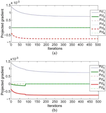
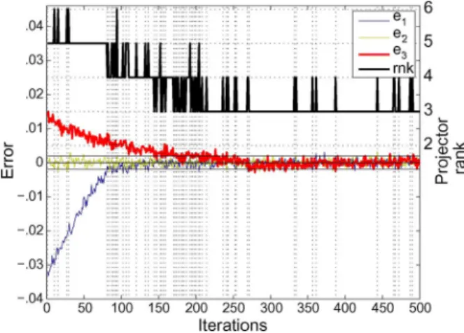
Fig. 5. Experiment A: main task error and projection operator rank using the directional redundancy formalism. The rank of the projection operator is not constant during the servo. At the beginning of the servo, the DOF corresponding to Componentse and e are available for the secondary task. The projection operator rank is thus 5. The DOF corresponding toe is used by the secondary task. The decrease is thus faster than required by the main task. Whene be-comes null, the projection operator rank decreases (Iteration 80). The DOF cor-responding toe is available until Iteration 300. At this instant, the main task error is null. No additional DOF remains free. The projection operator is thus the same than the one obtained by the classical formalism.
Fig. 6. Experiment A: comparison of the projected secondary task using the classical and the directional redundancy formalism. While the first component of the main task is not null (until Iteration 80), two components of the secondary tasks are taken into account using the directional redundancy formalism, but nullified by the classical formalism. (a) Classical redundancy formalism; (b) directional redundancy formalism.
law, and proposes a simple hysteresis comparator to filter the noise when computing the projection operator.
1) Comparison With the Classical Redundancy Formalism:
Using the classical redundancy formalism, the projection-oper-ator rank is 3 during the whole execution (see Fig. 4). The error behavior is a perfect exponential decrease, as specified by .
Fig. 7. Experiment A: control law using the directional redundancy formalism. The norm of the translational and rotational velocities are represented. The ve-locity changes at Iteration 80, corresponding to the projection-operator rank de-crease (see Fig. 5).
On the contrary, when using the formalism proposed above, the projection-operator rank is greater than 3 while the error of the main task is not null. As can be seen on Fig. 5, the convergence of the first component of the main-task error is accelerated by the secondary task. When it reaches 0, the projection operator looses a rank. The third component of the error does not cor-respond to any part of the secondary task, and is thus let un-touched. The corresponding DOF is available but not used by the secondary task. When reaches 0, the projection operator looses another rank. From this point, there is no difference at all between the two redundancy formalisms: the two projection operators are equal, and the robot behavior is the same.
The effect of the projection operator on the secondary task is shown in Fig. 6. While Component is not null, a part of the secondary task is nullified by the classical projection operator, but taken into account by the proposed control law. Intuitively, the main task is composed of two parts: centering and zooming. Since the secondary task is a translation along X-axis, it modi-fies the centering. When the main task is realized, the projection operator mainly generates an artificial rotation to compen-sate the secondary velocity and thus preserves the centering. In the initial configuration presented here, the secondary task has an acceptable influence on the centering, since it helps to realize the centering. It is thus accepted when using the direc-tional redundancy formalism while the object is not centered in the image. As soon as the centering is realized, the part of the secondary task that modifies the centering is rejected, and nul-lified by the projection operator. Component which is part of the centering converges thus faster than using the classical redundancy formalism. The DOF corresponding to the zoom is also available using the directional redundancy. However, since the secondary task has no effect on the zoom, it is not used and Component of the main task which corresponds to the zoom converges like when using the classical formalism.
2) In Presence of Noise: A white noise is added directly
to the computation of the main-task error. The error will thus never reach . The task is considered to be completed when it is smaller than a threshold equals to the variance of the noise. The computation of the projection operator also requires to test if the components of the error is null: a DOF is available when the corresponding error component is not null but disappears
Fig. 8. Experiment A: main task error and projection operator rank using the di-rectional redundancy formalism in the presence of noise without any hysteresis comparator. The projection operator rank increases each time an error compo-nent passes through the threshold.
Fig. 9. Experiment A: control law using the directional redundancy formalism in the presence of noise without any hysteresis comparator. A peak appears each time the projection operator rank increases.
as soon as the component reaches 0 (see (33)). Once again, the error component is considered null if it is smaller than the noise variance.
The main task error and the rank of the projection operator are given in Fig. 8. As can be seen on this figure, the rank of the operator is very noisy. Since the rank is discrete, the white noise is amplified when computing the projection operator and induces thus a very strong perturbation: each time the error in-creases above the threshold because of the noise, the projection operator rank increases. As can be seen on Fig. 9, the noise is amplified by the control law computation and a lot of strong dis-continuities appear in the control law.
3) Hysteresis Comparator: The problem is solved using
a simple principle known as the Schmitt trigger in electrical engineering [22]. Two thresholds are used to determine if the error is null. The output of the comparison is not null if the error is greater than the higher threshold; the output is null if the error is smaller than the lower threshold. And when the error is between the two thresholds, the output retains the previous value. The lower threshold is set to the noise variance, which corresponds to one standard deviation. The higher threshold has to be set so that an error greater than the threshold has a very low probability to be only due to noise. We have set it to three standard deviations of the noise, which correspond
Fig. 10. Experiment A: main task error and projection operator rank using the directional redundancy formalism in the presence of noise using an hysteresis comparator. When an error component becomes less than the first threshold, the projection operator decreases. It will increase only if the corresponding error component increases above a second higher threshold. The projection operator is not noisy any more. Like in the non-noisy experiment, it decreases a first time whene becomes null (Iteration 70) and a second time when e becomes null (Iteration 140).
Fig. 11. Experiment A: control law using the directional redundancy formalism in the presence of noise using an hysteresis comparator. The control law is not discontinuous any more. The noise in the control law is due to the noise in the sensor measures, and is equivalent to the noise that we have set in input. The control law computation does not amplify the noise.
numerically to a probability of false detection approximately equals to 99.7%.
The results of the simulation using the hysteresis system are presented in Figs. 10–12. The projection operator rank is not noisy any more (see Fig. 10). The noise in the control law cor-responds to the noise on the error: the signal/noise ratio is no more amplified by the projection computation (see Fig. 11). The projected secondary task is given in Fig. 12. The values are very similar to the ones obtained without any noise (given on Fig. 6(b)). This emphasizes that the hysteresis comparator has removed the major part of the noise when computing the pro-jection operator.
In the following real experiments, the hysteresis comparator has also been used. The two thresholds could be set by a fastid-ious analysis of the probability distribution of the sensor mea-sures (the image processing in our case). We have assumed a Gaussian distribution. The variance has then been computed from experimental results directly and the same two thresholds as mentioned above have been used.
Fig. 12. Experiment A: projected secondary task using the directional redun-dancy formalism in the presence of noise using an hysteresis comparator. The projected secondary task is very similar to the one obtained without noise (see Fig. 6(b)). The projection operator is thus robust to the noise in the sensor measure.
Fig. 13. Experiment B: joint trajectories of the two first components of the joint vector. It corresponds mainly to the camera position in the planeXY . The joint limits are represented in red. The trajectory with the classical redundancy formalism is represented in yellow. It ends in the joint limits. The trajectory with the proposed method is in blue. The positioning task succeeds (s is reached).
B. First Experiment on the Robot (Six DOF Constrained)
The two next experiments have been realized on a six-DOF eye-in-hand robot. In this experiment, the robot has to reach a unique pose with respect to the visual target. The main task uses all the DOF of the robot. The projection operator computed using the classical redundancy formalism is thus null.
Thanks to the choice of adequate visual features, the camera trajectory without any secondary task is almost a straight line (it is not a perfect straight line because the features are not perfectly decoupled). Since the robot joint domain is not convex and the trajectory is close to a straight line, the robot reaches its joint limits during the servo. Since there is no DOF left using the classical redundancy formalism, the main task fails when the robot reaches its joint limits as shown in Fig. 13.
Using the method proposed above, the projection operator is not null as long as the error of the main task is not zero. Fig. 14 gives the rank of the projection matrix during the execution. When the robot is near the joint limits, the projection operator is not null and the projected gradient is also not null (see Fig. 15). The induced secondary control law is large enough to modify the trajectory imposed by the main task and to avoid the joint limits. Fig. 16 presents the evolution of three visual features
Fig. 14. Experiment B: rank of the projection operator computed using the proposed approach during the servo.
Fig. 15. Experiment B: projected gradient using the proposed method. The sec-ondary control law mainly increases the third component of the joint speed, that corresponds to the speed along the optical axis.
Fig. 16. Experiment B: evolution of the visual features when applying the pro-posed method. The two featuresx and a (plotted in red and blue) are modi-fied by the avoidance law. On the opposite, features (plotted in green) is not modified.
whose value is modified by the secondary control law. The pro-jection operator mainly accelerates the decreasing speed of fea-tures and controlling the centering (pan) and the motion along the optical axis. Using the framework presented above, it is thus possible to free up some additional DOF that are not available within the classical redundancy formalism. The main task is correctly completed, and the servo is not slowed by the secondary control law.
C. Second Experiment on the Robot (Four DOF Constrained)
In the previous experiment, no avoidance law could be taken into account by the classical redundancy formalism. It was thus
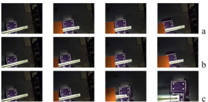
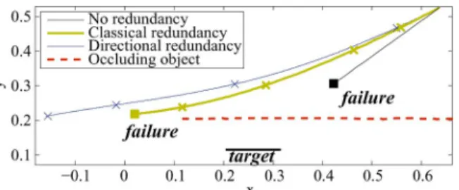
Fig. 17. Experiment C: main phases of the servo (a) without avoidance, (b) with the avoidance law projected using the classical redundancy formalism, and (c) using the directional redundancy. The pictures are taken by the embedded camera. The visual target is the four-white-points rectangle. The occluding object is the orange shape that appears in the left of the image.
Fig. 18. Experiment C: norms of the projected gradient using the classical re-dundancy formalism (yellow) and of the projected gradient using the proposed approach (blue). The projected gradient using the classical framework is lower than the one obtained with our method.
easy to see that the performance of our framework is better. The next experiment will point out that, even when DOF are avail-able for avoidance, a better behavior of the system is obtained by considering a larger free space as done above.
The main task is composed of four visual features. The robot has to move in order to center the object in the image, to rotate it properly around the optical axis, and to bring the camera at a distance of 1.5 m of the target using . Two DOF are thus available, that correspond mainly to motions on a sphere whose center is the target. During the servo, an object moves between the camera and the visual target, leading to an occlusion. The two available DOF are used to avoid this occlu-sion, as explained in Section V-C-2.
Without any avoidance law, the visual target is quickly oc-cluded, which makes the servo to fail [Fig. 17(a)]. Using the classical redundancy formalism, the gradient is projected into a two-dimensional space. Its norm is thus reduced, and the sec-ondary control law is not fast enough to avoid the occlusion. Mainly, the projection operator forbids the motion along the optical axis, which is controlled by one of the features of the main task (Fig. 18). This motion is available using our approach (Fig. 19). The robot velocity is thus fast enough to avoid the oc-clusion [Fig. 17(c)]. The decreasing speed of some visual fea-tures has been accelerated to enlarge the free space of the first task (Fig. 20). When the occlusion ends, the features decrease is no longer modified. The trajectory of the camera is given in Fig. 21. When the occlusion is not taken into account, the tra-jectory is a straight line. When taking the occlusion into account using the classical redundancy formalism, the additional motion
Fig. 19. Experiment C: translational velocities of the avoidance control law projected using the classical redundancy formalism (a) and projected using the proposed approach (b). The motions along the camera axis (red) are not null using the proposed control law.
Fig. 20. Experiment C: decreasing error of the visual features. The occlusion avoidance begins at Event 1. The decrease of the feature plotted in red is accel-erated. The occlusion is completely avoided after Event 2. The decrease goes back to a normal behavior.
Fig. 21. Experiment C: comparison of the trajectory of the robot in the plane perpendicular to the target.
induces a translation that modifies the trajectory. When the di-rectional redundancy is used, the robot mainly accelerates the translation toward the camera.
VII. CONCLUSION
In this paper, we have proposed a new general method to inte-grate a secondary term to a first task having priority. Our frame-work is based on a generalization of the classical redundancy for-malism. We have shown that it is possible to enlarge the number of the available DOF, and thus to improve the performance of the avoidance control law. This control scheme has been validated in simulation and on a six-DOF eye-in-hand robotic platform where the robot had to reach a specific pose with respect to a visual target, and to avoid joint limits and occlusions.
We have shown that it is possible to find DOF during the accomplishment of a full-constraining task, and to enhance the avoidance process even when enough DOF are available.
Our current works aim at realizing a reactive servo, able to perform a full constraining task and to simultaneously take into account the perturbations due to a real robotic system. The gen-eral idea is to free up as many DOF as possible to perform the avoidance of any obstacle encountered during the servo [16]. Using the method proposed in this article, additional DOF are collected at the very bottom level, directly in the control law. An avoidance can be realized even when the adequate DOF are al-ready used by the main task. However, the number of DOF can be insufficient for example when the obstacles are numerous. We now focus on the choice of the main task, to obtain addi-tional DOF by modifying the main task from a higher level.
ACKNOWLEDGMENT
The authors would like to thank the anonymous reviewers for their valuable comments which allow great improvements in the clarity and presentation of the paper.
REFERENCES
[1] P. Baerlocher and R. Boulic, “An inverse kinematic architecture en-forcing an arbitrary number of strict priority levels,” Visual Comput., vol. 6, no. 20, pp. 402–417, Aug. 2004.
[2] A. Ben-Israel and T. Greville, Generalized Inverses: Theory and
Ap-plications. New York: Wiley-Interscience, 1974.
[3] T. Chang and R. Dubey, “A weighted least-norm solution based scheme for avoiding joints limits for redundant manipulators,” IEEE
Trans. Robot. Automat., vol. 11, no. 2, pp. 286–292, Apr. 1995.
[4] F. Chaumette and S. Hutchinson, “Visual servo control, part i: Basic approaches,” IEEE Robot. Automat. Mag., vol. 13, no. 4, pp. 82–90, Dec. 2006.
[5] F. Chaumette and E. Marchand, “A redundancy-based iterative scheme for avoiding joint limits: Application to visual servoing,” IEEE Trans.
Robot. Automat., vol. 17, no. 5, pp. 719–730, Oct. 2001.
[6] N. Cowan, J. Weingarten, and D. Koditschek, “Visual servoing via nav-igation functions,” IEEE Trans. Robot. Automat., vol. 18, no. 4, pp. 521–533, Aug. 2002.
[7] B. Espiau, F. Chaumette, and P. Rives, “A new approach to visual servoing in robotics,” IEEE Trans. Robot. Automat., vol. 8, no. 3, pp. 313–326, Jun. 1992.
[8] J. Feddema and O. Mitchell, “Vision-guided servoing with feature-based trajectory generation,” IEEE Trans. Robot. Automat., vol. 5, no. 5, pp. 691–700, Oct. 1989.
[9] G. Hager, “Human-machine cooperative manipulation with vi-sion-based motion constraints,” in Proc. Workshop Visual Servoing,
IEEE/RSJ Int. Conf. Intell. Robot. Syst. (IROS’02), Lausane,
Switzer-land, Oct. 2002, [CD ROM].
[10] H. Hanafusa, T. Yoshikawa, and Y. Nakamura, “Analysis and control of articulated robot with redundancy,” in Proc. IFAC, 8th Triennal World
Congress, Kyoto, Japan, 1981, vol. 4, pp. 1927–1932.
[11] Visual Servoing: Real Time Control of Robot Manipulators Based on
Visual Sensory Feedback, K. Hashimoto, Ed. Singapore: World Sci-entific, 1993, vol. 7.
[12] S. Hutchinson, G. Hager, and P. Corke, “A tutorial on visual servo control,” IEEE Trans. Robot. Automat., vol. 12, no. 5, pp. 651–670, Oct. 1996.
[13] O. Khatib, “Real-time obstacle avoidance for manipulators and mobile robots,” Int. J. Robot. Res., vol. 5, no. 1, pp. 90–98, Spring, 1986. [14] C. Klein and S. Kittivatcharapong, “Optimal force distribution for the
legs of a walking machine with friction cone constraints,” IEEE Trans.
Robot. Automat., vol. 6, no. 1, pp. 73–85, Feb. 1990.
[15] A. Liégeois, “Automatic supervisory control of the configuration and behavior of multibody mechanisms,” IEEE Trans. Syst., Man Cybern., vol. 7, no. 12, pp. 868–871, Dec. 1977.
[16] N. Mansard and F. Chaumette, “Task sequencing for sensor-based con-trol,” IEEE Trans. Robotics, vol. 23, no. 1, pp. 60–72, Feb. 2007. [17] E. Marchand and G. Hager, “Dynamic sensor planning in visual
ser-voing,” in Proc. IEEE/RSJ Int. Conf. Intell. Robot. Syst. (IROS’98), Leuven, Belgium, May 1998, pp. 1988–1993.
[18] Y. Mezouar and F. Chaumette, “Path planning for robust image-based control,” IEEE Trans. Robot. Automat., vol. 18, no. 4, pp. 534–549, Aug. 2002.
[19] B. Nelson and P. Khosla, “Strategies for increasing the tracking region of an eye-in-hand system by singularity and joint limits avoidance,” Int.
J. Robot. Res., vol. 14, no. 3, pp. 255–269, Jun. 1995.
[20] J. Rosen, “The gradient projection method for nonlinear program-mimg, part i, linear constraints,” SIAM J. Appl. Math., vol. 8, no. 1, pp. 181–217, Mar. 1960.
[21] C. Samson, M. Le Borgne, and B. Espiau, Robot Control: The Task
Function Approach. Oxford, U.K.: Clarendon Press, 1991. [22] O. Schmitt, “A thermionic trigger,” J. Scientific Instrum., vol. 15, pp.
24–26, 1938.
[23] O. Tahri and F. Chaumette, “Point-based and region-based image mo-ments for visual servoing of planar objects,” IEEE Trans. Robotics, vol. 21, no. 6, pp. 1116–1127, Dec. 2005.
Nicolas Mansard graduated from École Nationale
Supérieure d’Informatique et de Mathématiques Appliquées, Grenoble, France and received the M.S. (DEA) degree in robotics and image processing from the University Joseph Fourier, Grenoble, in 2003 and the Ph.D. degree in computer science from the University of Rennes, Rennes, France, in 2006.
He spent three years in the Lagadic research group, IRISA, INRIA-Bretagne. He then spent one year at Stanford University, Stanford, CA, and one year with JRL-Japan, AIST, Tsukuba, Japan. He is currently with LAAS/CNRS, Toulouse, France, in the GEPETTO group. His research interests are concerned with sensor-based robot animation, and more specifi-cally the integration of reactive control schemes into real robot and humanoid applications.
Dr. Mansard received the Best Thesis Award from the French Research Group GdR-MACS, in 2006, the Best Thesis Award from the Society for Telecomu-nication and Computer Science (ASTI), in 2007, and the Best Thesis Award of the Région Bretagne.
François Chaumette (M’98) received the M.S.
de-gree from École Nationale Supérieure de Mécanique, Nantes, France, in 1987 and the Ph.D. degree in com-puter science from the University of Rennes, Rennes, France, in 1990.
Since 1990, he has been with IRISA/INRIA Rennes Bretagne Atlantique, where he is “Directeur de recherche” and Head of the Lagadic Group. He is the coauthor of more than 50 papers published in international journals on the topics of robotics and computer vision. His research interests include robotics and computer vision, especially visual servoing and active perception. Dr. Chaumette received several awards including the AFCET/CNRS Prize for the Best French Thesis on Automatic Control in 1991 and the King-Sun Fu Memorial Best IEEE TRANSACTIONS ONROBOTICS ANDAUTOMATIONPaper Award in 2002. He has been the Associate Editor of the IEEE TRANSACTIONS ONROBOTICSfrom 2001 to 2005 and is now in the Editorial Board of the
Inter-national Journal of Robotics Research. He has served over the last five years on
the program committees for the main conferences related to robotics and com-puter vision.