HAL Id: hal-01241477
https://hal-ensta-bretagne.archives-ouvertes.fr/hal-01241477
Submitted on 23 Feb 2016
HAL is a multi-disciplinary open access
archive for the deposit and dissemination of
sci-entific research documents, whether they are
pub-lished or not. The documents may come from
teaching and research institutions in France or
L’archive ouverte pluridisciplinaire HAL, est
destinée au dépôt et à la diffusion de documents
scientifiques de niveau recherche, publiés ou non,
émanant des établissements d’enseignement et de
recherche français ou étrangers, des laboratoires
ISAR Image formation with a combined Empirical Mode
Decomposition and Time-Frequency Representation
Ahmed Hadj Bay Ahmed, Jean-Christophe Cexus, Abdelmalek Toumi
To cite this version:
Ahmed Hadj Bay Ahmed, Jean-Christophe Cexus, Abdelmalek Toumi. ISAR Image formation with
a combined Empirical Mode Decomposition and Time-Frequency Representation. EUSIPCO, Aug
2015, Nice, France. pp.1366-1370. �hal-01241477�
ISAR IMAGE FORMATION WITH A COMBINED EMPIRICAL MODE DECOMPOSITION
AND TIME FREQUENCY REPRESENTATION
Bay Ahmed Hadj Ahmed
∗†, Jean-Christophe Cexus
∗, Abdelmalek Toumi
∗∗
Lab-STICC, UMR CNRS 6285,
ENSTA Bretagne
2, rue Franc¸ois Verny,
29806 Brest Cedex 9, France.
email: {cexusje, toumiab}@ensta-bretagne.fr
†
IRENav, EA3634,
Ecole Navale
BCRM Brest, CC 600,
29240 Brest Cedex 9, France.
email: hadj ahmed.bay [email protected]
ABSTRACT
In this paper, a method for Inverse Synthetic Aperture Radar (ISAR) image formation based on the use of the Complex Empirical Mode Decomposition (CEMD) is proposed. The CEMD [1] which based on the Empirical Mode Decompo-sition (EMD) is used in conjunction with a Time-Frequency Representation (TFR) to estimate a 3-D time-range-Doppler Cubic image, which we can use to effectively extract a se-quence of ISAR 2-D range-Doppler images. The potential of the proposed method to construct ISAR image is illustrated by simulations results performed on synthetic data and com-pared to 2-D Fourier Transform and TFR methods. The simu-lation results indicate that this method can provide ISAR im-ages with a good resolution. These results demonstrate the potential application of the proposed method for ISAR image formation.
Index Terms— Inverse Synthetic Aperture Radar, Image formation, Complex Empirical Mode Decomposition, Time-Frequency Representation.
1. INTRODUCTION
Nowadays in signal processing, spectrum analysis plays a key role to characterize and understand many phenomena and es-pecially for Radar systems such as the Inverse Synthetic Aper-ture Radar (ISAR). However, for a non-stationary signal, the frequency components can appear or disappear. To deal with these temporal evolutions, a Time-Frequency Analysis must be considered [2, 3]. The reconstruction process of ISAR image exploit the target’s motions. Thus, ISAR images are usually obtained by the range-Doppler algorithm based on the 2-D Fourier Transform to convert the data in the tial frequency domain to reflectivity information in the spa-tial domain. However, because of the target maneuvering, the Doppler spectrum becomes time-varying and the image is blurred. Instead of the Fourier Transform, TFR techniques can be adopted to improve the resolution of ISAR images [3–5]. In recent years, a great deal of interest has been paid
to transformations or processing that map the signal into its TFR [5–7].
Recently, Empirical Mode Decomposition (EMD) has been introduced by Huang et al. [8] for analyzing data from non-stationary and nonlinear processes. It is a new local and fully data-driven method for the multiscale analysis of nonlinear and non-stationary real-world signals. Hence, the analysis is self-adaptive in contrast to the traditional methods where the basis functions are fixed [9]. The EMD is based on the sequential extraction of energy associated with various in-trinsic time scales of the signal, called Inin-trinsic Mode Func-tions (IMF). The EMD has received more attention in terms of interpretations [10, 11], improvement [1, 12–14], Time-Frequency Analysis [15–17], denoising [18, 19], Speech enhancement [20], and Radar field [21–25] . . . .
In this present work, we investigate an approach based on CEMD and TFR, called CEMD-TFR, for ISAR image con-struction. The paper is organized as follows. In section 2, we briefly review the EMD algorithm of real-valued data, and describe several extensions methods to the complex domain in order to handle the complex ISAR raw data. Section 3 gives an overview of ISAR formation with Time-Frequency Representation and the method based on EMD-TFR. Some simulations and comments are proposed in section 4. Finally, the last section gives some conclusions and remarks.
2. METHOD DESCRIPTION 2.1. EMD algorithm
The EMD method decomposes a signal x(t) into a finite set of oscillatory modes, called Intrinsic Mode Functions (IMF), through an iterative process called sifting algorithm [8]. The name IMF is adopted because it represents the fast to the slow oscillations in the signal. The IMF represent the natural oscil-latory mode embedded in signal and work as the basis func-tions. Usually, an IMF can be both amplitude and frequency modulated (AM-FM). The essence of the EMD is to identify the IMF in different time scales, which can be defined locally
by the time lapse between two extrema of an oscillatory mode or by the time lapse between two zero crossings of such mode. The EMD picks out the highest frequency oscillation that re-mains in the signal. Thus, locally, each IMF contains lower frequency oscillations than the one extracted just before. The EMD decomposes a signal into a sum of IMF that : (R1) have the same number of zeros crossings and extrema; and (R2) are symmetric with respect to the local mean. The procedure used for extraction of an IMF from signal x(t) is outlined in algorithm :
Algorithm : EMD.
Step 1. Find the location of all local maxima/minima of x(t).
Step 2. Compute Upper (U (t)) and Lower (L(t)) envelope
by interpolating using cubic spline, respectively local maxima and minima.
Step 3. Compute the local mean envelope :
µ(t) = [U (t) + L(t)]/2 .
Step 4. Subtract the local mean from the signal to obtain the
oscillatory mode : h(t) ← x(t) − µ(t).
Step 5. Compute the stopping criteria SD :
if h(t) obeys the stopping criteria SD, then h(t) is an IMF otherwise set x(t) ← h(t) and repeat the process from Step 1.
Once the first IMF is estimated, the same process is applied to the residual x(t) − h(t) to extract the remaining IMFs. The sifting is also repeated several times in order to get h(t) as to be a true IMF that fulfills the requirements (R1) and (R2). The result of the sifting procedure is that x(t) will be decomposed
into IM Fj(t), j = 1, . . . N and residual rN(t) :
x(t) =
N
X
j=1
IM Fj(t) + rN(t). (1)
The total sum of the IMFs matches the signal very well
and therefore ensures completeness [8]. The sifting
pro-cess has two effects: (a) eliminates riding waves and (b) smooth uneven amplitudes. To guarantee that the IMF com-ponents retain enough physical sens of both AM and FM informations, the stop criterion is originally based on the normalization squared difference between two successive sifting iterations [8]. It should be noted that there are other more robust criterion based upon the original definition of IMF [10, 11].
2.2. Complex extension of EMD
The original EMD can only be applied to real-valued time se-ries, so it is necessary to extend the EMD to the complex do-main. Despite original EMD becoming a standard for Time-Frequency analysis of nonlinear and non-stationary signals, its multivariate extensions, especially on complex signals (or images), are only emerging. Different methods have been
proposed such as RIEMD [26], BEMD [12] and CEMD [1]. Besides these approaches, the extensions to trivariate and multivariate methods have also been developed and applied successfully [13, 14, 25, 27]. It should be noted that the recent advances in applications of micro-Doppler effects have been presented in radar area based on EMD [22, 25, 28].
In [26], the authors proposed a method called Rotation Invari-ant Empirical Mode Decomposition (RIEMD), which differs from the original EMD in the way of getting the extrema and the envelopes. The extrema were thought as the locus where the first derivative of the angle changes its sign, and the max-ima and minmax-ima were assumed to occur alternately. Then the cubic spline interpolation is performed directly in C to obtain the complex envelopes which are then averaged to obtain the local mean of signal. The other steps were same as the origi-nal EMD. This approach appears as a natural extension of real valued EMD.
In [12], Rilling et al. proposed another method termed Bivari-ate Empirical Mode Decomposition (BEMD) based on the idea of replacing the oscillation notion by a rotation notion. The complex signal was firstly projected to a certain direc-tions to extract the maxima of the projection vector, and then connected these points forming the upper envelope. Repeat projecting the complex signal to different directions to obtain the envelopes in different directions. This approach effec-tively sifts rapidly rotating signal components from the slowly rotating ones and uses the same complex cubic spline inter-polation scheme as RIEMD. It should be noted that BEDM algorithm calculates local mean envelope based on the ex-trema of both (real and imaginary) components of a com-plex signal and thus yielding more accurate estimates than RIEMD [26, 29].
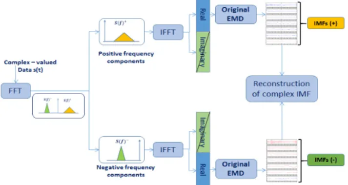
Fig. 1. Block diagram of CEMD algorithm.
In [1], the authors proposed a method named Complex Em-pirical Mode Decomposition (CEMD). This approach uses the inherent relationship between the positive and negative frequency components of a complex signal and the Hilbert Transform. Indeed, a complex signal has a asymmetric spec-trum and can be converted into a sum of two analytic signals by first separating the positive and negative frequency compo-nents of the spectrum and then converting back into the time domain (Figure 1). And subsequently, the original EMD is
applied to the two extracted signals. The algorithm has rig-orous mathematical background and it preserves the dyadic filter bank properties [1, 29]. However, this method cannot guarantee an equal number of real and imaginary IMFs. In the present work, this method was used because it seems more applicable to ISAR image construction.
3. TIME-FREQUENCY REPRESENTATION-BASED ISAR FORMATION
The common radar imaging method is based on the 2-D Fourier Transform (FT) and assumes that the Doppler fre-quency shifts must remain constant [3, 6]. If input complex data consists of M time history series, each one having length of N , then it should be noted that the 2-D FT based image formation generates only one image frame from M × N data array as shown in Figure 4(a). However, when the Doppler spectrum is time-varying due to target’s motion, ISAR image based on Fourier Transform becomes unclear and smeared. However, the joint Time-Frequency Transform can be used to enhance the ISAR images of moving targets [3, 4, 6].
3.1. ISAR imaging based on TFR
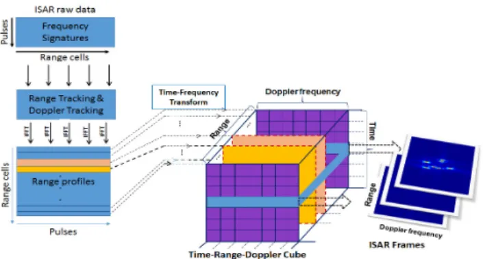
To compute a clear ISAR image of maneuvering targets, a Time-Frequency Transforms is always desirable. Figure 2 shows the radar imaging system based on the TFR [6].
Fig. 2. Block diagram of Time-Frequency based ISAR image formation.
It should be noted that the Time-Frequency Transform based image formation takes the TFR for each time history series and generates an N × N time-Doppler representations. By combining the M time-Doppler representations at M range cells, we obtain a cube with N × M × N time-range-Doppler values. There are also N images frames availables and ev-ery one represents a full range-Doppler images at a particular time instant. Therefore, by replacing the Fourier Transform with the TFR, a 2-D range-Doppler Fourier image frame be-comes a 3-D time-range-Doppler images cube. By sampling the image cube in time, a time sequence of 2-D range-Doppler images can be viewed. Each individual time-sampled frame
from the cube provides not only a clear image with superior resolution but also time-varying properties from one time to another. Different methods have been proposed for ISAR imaging using TFRs such as Cohen class Time-Frequency distribution [3, 4, 6], S-Transform [5, 7] or Harmonic Wavelet [30].
3.2. ISAR imaging based on EMD-TFR
The approach of the present work combines the CEMD to TFR as Spectrogram, Wigner-Ville Distribution (WVD) or Smoothed Pseudo Wigner-Ville Distribution (SPWVD). The CEMD-TFR method can be divided into two parts. The first one deals with the separation of the signal into IMFs using the CEMD. In second part, the Time-Frequency Analysis is applied on the separated components (IMFs) using Spectro-gram, WVD or SPWVD (Figure 3).
Fig. 3. Block diagram of CEMD-TFR algorithm based ISAR image formation.
Thus, the EMD is used as a multiband ltering to separate each components in the temporal domain before applying TFR. The intrinsic mode functions are used to construct a series of views by highlighting concentrations of energy in Time-Frequency domain. Therefore, we obtain a composite TFR based on a multiple views for each range profile signal. The advantage of such a method is that it can overcome interfer-ence in TFRs generated by the existinterfer-ence of multiple signal components. Once all TFRs associated with each IMF for a unique range cell are obtained, we compute a unique TFR (as a simple sum). Actually, the final result is an energy TFR at each range cell and along pulses, and time-Doppler spectrum is estimated. Then, by combining the time-Doppler spectrum at all range cells, we obtain a 3-D time-range-Doppler cu-bic image. Finally, the last step of classical image formation based on TFR is applied and a sequence of 2-D range Doppler images can be extracted.
4. RESULTS
We tested our approach on the simulated MIG25 dataset de-scribed in [3, 6]. The simulated aircraft is composed of 120 point scatterers of equal reflectivity. The raw data contains
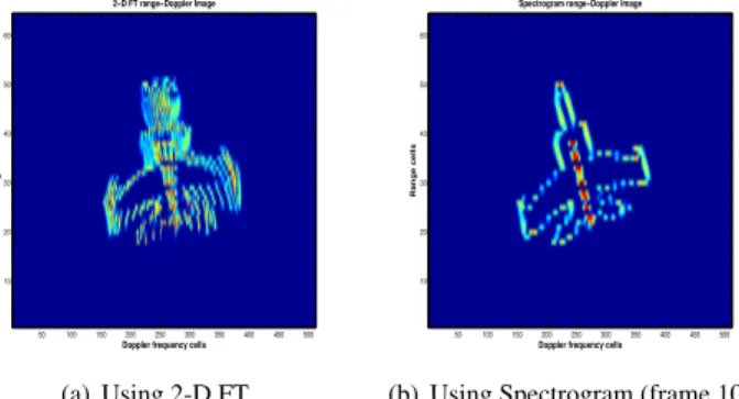
512 recurrences of 64 range bins. For all simulations, stan-dard motion compensation algorithm has been applied to the data. It should be noted that the representation of these fig-ures is in decibel. The EMD-TFR applied to the cross-range dimension significantly improves image readability as it is presented in the Figure 6 compared to the conventional 2-D Fourier Transform (FT) (Figure 4(a)), Spectrogram (Figure 4(b)) and RTF (Figure 5). Figure 5(a) shows the ISAR im-age formation using WVD. The blurring effects due to the cross-term interference associated with the WVD are evident. To reduce the cross term interference, the SPWVD (Figure 5(b)) can be used to preserve TFR properties with slightly re-duced time-frequency resolution and largely rere-duced cross-term interference. Comparing the EMD-WVD against the WVD, we see that in the figure 6(b) the components are well estimated and reduced cross-term interference with a good resolution. The simulation results show that this EMD-TFR can improve the constructed image compared with the Fourier Transform method. The EMD-TFR provides very interesting performance when the Time-Frequency energy is presented by the concentration and resolution of TFR along the indi-vidual component of the multi-components (non-stationary) signals.
Doppler frequency cells
Range cells 2−D FT range−Doppler Image 50 100 150 200 250 300 350 400 450 500 10 20 30 40 50 60 (a) Using 2-D FT.
Doppler frequency cells
Range cells
Spectrogram range−Doppler Image
50 100 150 200 250 300 350 400 450 500 10 20 30 40 50 60
(b) Using Spectrogram (frame 10). Fig. 4. Comparison of 2-D FT and Spectrogram based image.
Doppler frequency cells
Range cells WVD range−Doppler Image 100 200 300 400 500 600 700 800 900 1000 10 20 30 40 50 60
(a) Using WVD (frame 10).
Doppler frequency cells
Range cells SPWVD range−Doppler Image 100 200 300 400 500 600 700 800 900 1000 10 20 30 40 50 60 (b) Using SPWVD (frame 10). Fig. 5. Comparison of Time-Frequency based image.
5. CONCLUSIONS
In this paper, a new method of ISAR image formation based on EMD and TFR is proposed in order to improve the ISAR
Doppler frequency cells
Range cells
EMD−Spectrogram range−Doppler Image
50 100 150 200 250 300 350 400 450 500 10 20 30 40 50 60
(a) Using EMD-Spectrogram (frame 10).
Doppler frequency cells
Range cells
EMD−WVD range−Doppler Image
100 200 300 400 500 600 700 800 900 1000 10 20 30 40 50 60
(b) Using EMD-WVD (frame 10).
Doppler frequency cells
Range cells
EMD−SPWVD range−Doppler Image
100 200 300 400 500 600 700 800 900 1000 10 20 30 40 50 60
(c) Using EMD-SPWVD (frame 10). Fig. 6. Comparison of EMD-TFR based image.
image resolution. The performance of the proposed method is compared with 2-D Fourier Transform method as well as conventional TFR methods (Spectrogram, WVD, SPWVD). The effectiveness of this approach has been veried with simu-lated data from a non-cooperative target. The obtained results show that the proposed approach is an effective and a promis-ing imagpromis-ing method for ISAR image formation. Nevertheless, this technique is empirical, so further theoretical explanation work is needed and a large class of data are necessary to con-firm the obtained results. As future work, we plane to study the EMD-TFR in noisy environment and we intend to address the general decision-making process (classification problem and target identification). It seems also to be interesting to use others TFR such as the Huang-Hilbert Transform [8] or the Teager-Huang Transform [15].
REFERENCES
[1] T. Tanaka, and D.P. Mandic, ”Complex Empirical Mode Decomposition,” IEEE Signal Processing Letters, vol. 14(2), pp. 101-104, 2006.
[2] L. Cohen, ”Time-frequency analysis: theory and ap-plications,” Prentice-Hall, Englewood Cliffs, NJ, USA, 299 pages, 1995.
[3] V.C. Chen, and H. Ling, ”Time-Frequency Transforms for Radar Imaging and Signal Analysis,” Artech House,
Boston,232 pages, 2002.
[4] V. Corretja, E. Grivel, et al., ”Enhanced Cohen class Time-Frequency methods based on a structure tensor
analysis: Applications to ISAR processing,” Signal
Processing,vol. 93(7), pp. 1813-1830, 2013.
[5] I. Djurovic, L. Stankovic, et al., ”Time-Frequency Analysis for SAR and ISAR Imaging,” GeoSpatial
Vi-sual Analytics, Springer,pp. 113-127, 2009.
[6] V.C. Chen, and M. Martorella, ”Inverse Synthetic Aper-ture Radar Imaging; Principles, Algorithms and Appli-cations,” SciTech Publishing, 289 pages, 2014.
[7] L.J. Stankovic, T. Thayaparan, et al., ”S-method in Radar Imaging,” EUSIPCO’06, 5 pages, 2006.
[8] N.E. Huang, Z. Shen, et al., ”The Empirical Mode De-composition and the Hilbert spectrum for nonlinear and non-stationary time series analysis,” Proceedings of the
Royal Society, A,vol. 454, pp. 903-995, 1998.
[9] P. Flandrin, G. Rilling, and P. Goncalves, ”Empirical Mode Decomposition as a Filter Bank,” IEEE Signal
Processing Letters,vol. 11(2), pp. 112-114, 2004.
[10] N.E. Huang, M.L.C Wu, et al., ”A confidence limit for the Empirical Mode Decomposition and Hilbert spec-tral analysis,” Proceedings of the Royal Society, A, vol. 459, pp. 2317-2345, 2003.
[11] G. Rilling, P. Flandrin, and P. Goncalves, ”On Empiri-cal Mode Decomposition and its algorithms,” EURASIP workshop on nonlinear signal and image processing, NSIP-03, vol. 3, pp.8-11, 2003.
[12] G. Rilling, P. Flandrin, P. Goncalves, and J.M. Lilly, ”Bivariate Empirical Mode Decomposition,” IEEE
Sig-nal Processing Letters,vol. 14(12), pp. 936-939, 2007.
[13] N. Rehman, and D.P. Mandic, ”Multivariate Empirical Mode Decomposition,” Proceedings of the Royal
Soci-ety, A,vol. 466, pp. 1291-1302, 2009.
[14] M.H. Yeh, ”The complex bidimensional Empirical Mode Decomposition,” Signal Processing, vol. 92(2), pp. 523-541, 2012.
[15] J.C. Cexus, and A.O. Boudraa, ”Non-stationary sig-nals analysis by Teager-Huang Transform (THT),” EU-SIPCO’06, 5 pages, 2006.
[16] A. Bouchikhi, A.O. Boudraa, J.C. Cexus, and T. Chonavel, ”Analysis of multicomponent LFM signals by Teager Huang-Hough Transform,” Aerospace and
Electronic Systems, IEEE Transactions on, vol. 50(2),
pp. 1222-1233, 2014.
[17] N.J. Stevenson, M. Mesbah, and B. Boashash,
”Multiple-view time-frequency distribution based on the Empirical Mode Decomposition,” IET signal
pro-cessing,vol. 4(4), pp. 447-456, 2010.
[18] A.O. Boudraa, and J.C. Cexus, ”EMD-Based Signal Filtering,” Instrumentation and Measurement, IEEE
Transactions on,vol. 56(6), pp.2196-2202, 2007.
[19] P. Flandrin, P. Goncalves, and G. Rilling, ”Detrending and denoising with Empirical Mode Decomposition,” EUSIPCO’04,, 4 pages, 2004.
[20] K. Khaldi, A.O. Boudraa, A. Bouchikhi, and M.T. Alouane, ”Speech enhancement via EMD,” Journal on Advances in Signal Processing,, vol. 2008(1), 8 pages, 2008.
[21] H. Chunming, G. Huadong, W. Changlin, and F. Dian, ”A novel method to reduce speckle in SAR images,”
International Journal Remote Sensing,vol. 23(23), pp.
5095-5101, 2002.
[22] L. Du, B. Wang, Y. Li, and H. Liu, ”Robust classi-fication scheme for airplane targets with low resolu-tion radar based on EMD-CLEAN feature extracresolu-tion method,” IEEE Sensors Journal, vol. 13(12), pp. 4648-4662, 2013.
[23] B. Bjelica, M. Dakovic, et al.,”Complex Empirical De-composition method in radar signal processing,” Em-bedded Computing (MECO), 2012 Mediterranean Con-ference on, pp. 88-91, 2012
[24] Y. Yuani, M. Jin, et al., ”Empiric and dynamic detection of the sea bottom topography from synthetic aperture radar image,” Advances in Adaptive Data Analysis, vol. 1(2), pp. 243-263, 2009.
[25] J.H. Park, W. Y. Yang, et al., ”Extended high resolu-tion range profile-jet engine modularesolu-tion analysis with signal eccentricity,” Progress In Electromagnetics
Re-search,vol. 142, pp. 505-521, 2013.
[26] B. Altaf, M. Umair, et al., ”Rotation invariant com-plex Empirical Mode Decomposition,” ICASSP07, vol. 3, pp. 1009-1012, 2007.
[27] N.U. Rehman, and D.P. Mandic, ”Empirical mode de-composition for trivariate signals,” IEEE Transactions
on Signal Processing,vol. 58 (3), pp. 1059-1068,2010.]
[28] C. Cai, W. Liu, et al., ”Radar micro-Doppler signa-ture analysis with HHT,” IEEE Trans. Aerosp. Electron.
Syst.vol. 46(2), pp. 929-938, 2010.
[29] D.P. Mandic, and V.S.L. Goh, ”Complex Valued Non-linear Adaptive Filters: Noncircularity, Widely Linear and Neural Models,” John Wiley & Sons, 344 pages, 2009.
[30] B.K. Kumar, B. Prabhakar, et al., ”Target identification using harmonic wavelet based ISAR imaging,” Journal
on Applied Signal Processing, vol. 2006(1), pp. 1-13,