Université de Liège Faculté des Sciences
Dynamics of carbon dioxide and methane in the mangroves of Vietnam, and the rivers and the lagoons of Ivory Coast
Dynamique du dioxyde de carbone et du méthane dans les mangroves du Vietnam, les rivières et les lagunes de la Côte d’Ivoire
Dissertation présentée par
Yéfanlan José-Mathieu Koné
en vue de l’obtention du grade de Docteur en Sciences Novembre 2008
Travaux co-dirigés par
Dr A.V. Borges et Pr F. Ronday Jury :
Pr J.-M. Bouquegneau, Professeur à l'Université de Liège (Président du Jury) Dr A.V. Borges, Chercheur Qualifié au FNRS (Promoteur)
Pr F. Ronday, Administrateur de l'Université de Liège (Co-Promoteur) Pr A. Ouattara, Professeur à l'Université d’Abobo-Adjamé
Dr B. Delille, Chercheur à l'Université de Liège Dr G. Abril, Chargé de recherche au CNRS
Remerciements
Je tiens à adresser mes sincères remerciements au Professeur Jean-Marie Bouquegneau, qui a accepté d’être le président du jury de cette thèse de Doctorat. Je lui suis aussi très reconnaissant d’avoir été non seulement mon professeur d’océanographie biologique, mais aussi président de mon mémoire de DEA.
Je tiens à exprimer ma profonde gratitude au Docteur Alberto Vieira Borges promoteur de ce travail, qui m’a encadré pendant ces 6 dernières années. Il a mis tous les moyens à ma disposition, et ses connaissances approfondies en océanographie chimique, sa rigueur et sa qualité scientifiques. Je lui suis fort reconnaissant pour le temps qu’il m’a octroyé et surtout qu’il n’a pas hésité à me fournir les données qu'il avait lui-même collectées pour la réalisation de mon mémoire de DEA et également des données pour la finalisation de cette thèse. Merci aussi pour l’opportunité qu'il m'a offerte de participer au projet CARBO-OCEAN. Ce fut pour moi une très belle expérience que je garde en souvenir.
Je remercie également le Professeur François Ronday qui malgré ses nombreuses charges en tant qu’Administrateur de l’Université a accepté d’être co-promoteur de ce travail. Merci aussi pour les cours d’océanographie physique et de météorologie que vous nous avez donnés.
Une très grande reconnaissance au Docteur Bruno Delille qui s’est toujours montré très disponible, patient et pour tous ses nombreux coups de mains et ses conseils. A travers lui, je voudrais également dire merci à sa compagne Cécile et à ses enfants. Je me souviens que dans mes débuts à Liège, ils m’ont plusieurs fois reçu chez eux. Cela me reste à l’esprit. Merci aussi d’avoir accepté d’être membre de jury de ce travail.
Je tiens vivement à remercier le Docteur Gwenaël Abril de l’Université de Bordeaux 1 qui a accepté de collaborer au projet de l’Agence Universitaire de la Francophonie (AUF) et qui m’a aidé dans l’analyse et l’exploitation des données de méthane. Je lui suis très reconnaissant. Je lui dis également merci aussi d’avoir accepté d’être membre de jury de ce travail. A travers lui, je voudrais adresser mes sincères remerciements à Dominique Poirier qui a effectué les analyses de méthane. Je lui suis très reconnaissant.
Adjamé qui m’a beaucoup aidé lors de mes campagnes de terrain et qui a accepté aussi d’être membre de jury de ce travail. Merci pour ses nombreux conseils. A travers lui, je voudrais dire merci à tous les membres du Laboratoire d’Environnement et de Biologique Aquatique.
Une très grande reconnaissance va également à l’endroit du Professeur Gourène Germain, Vice-Président de l’Université d’Abobo-Adjamé qui a aussi accepté de collaborer au projet AUF et qui m’a offert un bureau pour le conditionnement de mes échantillons. Merci d’avoir mis toujours une voiture à notre disposition pour nos déplacements sur le terrain.
Je suis aussi reconnaissant au Docteur Steven Bouillon de la Katholieke Universiteit Leuven qui a accepté d’être membre de jury de ce travail dont les récents travaux sur les écosystèmes de mangroves m’ont permis d’avoir une vue plus large sur la dynamique du carbone dans ces milieux.
J'adresse également mes remerciements au Professeur Lei Chou, de l’Université Libre de Bruxelles (ULB) qui m’a accueilli dans son laboratoire pour l’analyse des nitrates. Je voudrais également dire merci à Jérôme, Caroline, Nathalie et à tous les autres membres du Laboratoire d'Océanographie Chimique de l’ULB.
Je suis aussi reconnaissant au Docteur Laure Sophie-Schiettecatte qui m’a aidé dans l’analyse des phosphates et de la silice. Je lui dis un grand merci pour les moments de joie qu’on a pu passer ensemble au laboratoire.
Je tiens vivement à remercier tous les autres membres de l’Unité d’Océanographie Chimique. Chacun de vous a contribué à sa manière, à l’élaboration de cette thèse. Merci à Kim dont la contribution m’a beaucoup aidé lors de mon séjour à Bruxelles pour l’analyse des nitrates. Un grand merci à mon ami Marc, à Nicolas et à Willy pour la bonne musique de chaque jour. J’ai été très heureux de les connaître et de passer ce temps avec eux au laboratoire.
Un grand merci à tous les membres du service UNIPC dont mon ami Olivier qui s’est toujours arrêté pour échanger quelques mots.
Je tiens aussi à remercier mes amis qui m’ont aidé à réaliser ce travail. Certains m’ont accompagné sur le terrain, je pense à Julie-Estelle Brou, Seu-Mireille Anoi, Norbert, Sylvestre, Aimé et Victor. Je dis surtout merci à Mireille pour l’attiéké de Frambo ! D’autres m’ont soutenu moralement, je pense à Paule-Marie, Zor et Stéphanie, Alain et Véronique,
Jean-Pierre et Cocco, Christian et Thérèse, Abel, Edia, Monique, Ferdinand, Ange et à mes petites sœurs Dorcas et Félicité.
Je voudrais aussi dire merci à tous mes oncles et mes tantes qui m’ont permis d’aller à l’école. Je leur suis très reconnaissant pour tout ce qu’ils ont fait pour moi durant toutes ces années. Un grand merci à ma famille adoptive à Daloa qui m’a manifesté un amour vraiment sans hypocrisie. Merci pour leurs bénédictions et prières qui m’ont rendu toujours plus joyeux.
Je suis aussi très reconnaissant envers toutes ces nombreuses personnes qui n’ont pas pu êtres citées dans ce document et qui par leurs petits gestes ont contribué à la réalisation de ce travail.
Enfin, s’il m’est permis, je voudrais rendre grâce à Dieu pour toutes choses.
Cette thèse a été effectuée au sein de l’Unité d’Océanographie Chimique de l’Université de Liège. Ce travail a été réalisé grâce à une bourse doctorale de l’Etat de la République de Côte d’Ivoire. C’est pourquoi je tiens à remercier infiniment les Autorités gouvernementales pour cette opportunité. L’Agence Universitaire de la Francophonie (convention n°6313PS657) et la Fondation Alice Seghers ont supporté les projets dans le cadre desquels j'ai effectué les missions de terrain. Le travail au Vietnam a été effectué avec le soutien du Fonds National de la Récherche Scientifique (FNRS). Je leur suis fort reconnaissant pour ces financements qui ont été essentiels pour la réalisation de ce travail.
Abstract
Tropical near-shore coastal ecosystems receive 60% of the world freshwater and an equivalent fraction of organic matter. Thus, these regions are expected to have a major role in the overall budgets of CO2 and CH4, two major greenhouse gases, in the coastal and global
oceans. As a contribution to the understanding of the role of the coastal ocean and continental aquatic environments in the global cycle of these gases, we report the seasonal variability of partial pressure of CO2 (pCO2), CH4 concentration, related air-water fluxes of CO2 and CH4
and ancillary data in several contrasted tropical coastal ecosystems in terms of geomorphology, lithology of the drainage basin, freshwater and seawater inputs, and riparian population and related anthropogenic pressure (land use change, aquaculture, waste waters release, eutrophication, and invasive species proliferation).
We investigated waters surrounding two forested mangrove sites (Tam Giang and Kiên Vàng) located in Ca Mau Province (South-West Vietnam), in five lagoons (Grand-Lahou, Ebrié, Potou, Aby and Tendo) and three rivers (Comoé, Bia and Tanoé) flowing into these lagoons in Ivory Coast.
Data from the two forested mangrove sites in South-West Vietnam were obtained during the dry and rainy seasons, providing for the first time information on the seasonality of dissolved inorganic carbon (DIC) and air-water CO2 fluxes in the water surrounding
mangrove ecosystems. Our data suggest an increase of heterotrophic activity in sediments and/or the water column during the rainy season that could be due to an increase of carbon inputs from soil flushing, probably from the land surrounding the mangrove forests. The air-water CO2 fluxes we computed are consistent with the few data available so far in waters
surrounding mangrove forests, and confirming that this emission of CO2 is significant for the
carbon budget of mangrove forests, and also for the regional CO2 budget at tropical and
sub-tropical latitudes.
Data in lagoons and rivers of Ivory Coast were obtained during four cruises covering the main climatic seasons (high dry season, high rainy season, low dry season and low rainy season). The three rivers were oversaturated in CO2 and CH4 with respect to atmospheric
equilibrium, and the seasonal variability of pCO2 and CH4 concentrations was due to dilution
aquatic compartment due to root respiration and organic matter degradation derived from these plants. However, floating macrophytes are atmospheric CO2 sinks.
The surface waters of the Potou, Ebrié and Grand-Lahou lagoons were oversaturated in CO2 and CH4 with respect to the atmosphere during all seasons. In contrast, the Aby and
Tendo lagoons exhibit enhanced over-saturation in CH4 but under-saturation in CO2 because
of their permanent haline stratification (unlike the other lagoons) that seemed to lead to higher phytoplankton production and export of organic carbon below the pycnocline. However, the permanent stratification also leads to anoxic bottom waters favorable to a large CH4
production. Thus, the largest CH4 over-saturations and diffusive air-water CH4 fluxes were
observed in the Tendo and Aby lagoons while they can act as a sink for atmospheric CO2. We
highlight the importance of physical settings (permanent versus seasonal stratification) in controlling the organic C flows, modulating the atmospheric CO2 source-sink status, and the
Résumé
Les écosystèmes côtiers tropicaux reçoivent 60% de l’eau douce mondiale et une fraction équivalente de la matière organique. Ainsi, ces régions sont supposées avoir un rôle important dans les budgets globaux de CO2 et de CH4, deux gaz à effets de serre majeurs,
dans les océans côtier et ouvert. Pour contribuer à la compréhension du rôle de l’océan côtier et des environnements aquatiques continentaux dans les cycles globaux de ces gaz, nous rapportons la variabilité saisonnière de la pression partielle de CO2 (pCO2), de la
concentration en CH4, des flux air-eau de CO2 et de CH4 ainsi que de certains paramètres
complémentaires dans plusieurs écosystèmes côtiers tropicaux contrastés en termes de géomorphologie, de lithologie du bassin versant, d'entrées d'eau douce et d'eau de mer, de populations avoisinantes et de la pression anthropique résultante (changement dans l'utilisation des sols, aquaculture, rejets d'eaux usées, eutrophisation et prolifération d'espèces invasives).
Nous avons étudiés les eaux entourant deux sites de forêts de mangroves (Tam Giang et Kiên Vàng) situés dans la Province de Ca Mau (sud-ouest du Vietnam), cinq lagunes (Grand-Lahou, Ebrié, Potou, Aby et Tendo) et trois rivières (Comoé, Bia et Tanoé) se jetant dans ces lagunes de Côte d’Ivoire.
Les données des deux sites de forêts de mangroves du sud-ouest du Vietnam ont été obtenues pendant les saisons sèche et pluvieuse, fournissant pour la première fois une information sur la variabilité saisonnière du carbone inorganique dissous (DIC) et des flux air-eau de CO2 dans des eaux entourant des écosystèmes de mangroves. Nos données montrent
une augmentation de l’activité hétérotrophe dans les sédiments et/ou dans la colonne d’eau pendant la saison pluvieuse qui pourrait être due à une augmentation des apports de carbone liés au lessivage des sols, probablement de la terre entourant les forêts de mangroves. Les flux air-eau de CO2 que nous avons calculés sont en accord avec les quelques rares données
disponibles dans les eaux entourant des forêts de mangroves, et confirment que les émissions du CO2 sont significatives par rapport au budget du carbone des forêts de mangroves, mais
aussi par rapport au budget régional des émissions de CO2 aux latitudes tropicales et
Les données dans les lagunes et des rivières de Côte d’Ivoire ont été obtenues pendant quatre campagnes couvrant les principales saisons climatiques (grande saison sèche, grande saison pluvieuse, petite saison sèche, petite saison pluvieuse). Les trois rivières étaient sursaturées en CO2 et en CH4 par rapport à l’équilibre atmosphérique, et la variabilité
saisonnière de la pCO2 et des concentrations du CH4 était liée à la dilution durant la période
de crue. Cependant, les espèces invasives de jacinthes flottantes Eichhornia crassipes qui recouvrent ces rivières peuvent être des contributrices significatives aux émissions de CO2
depuis le compartiment aquatique vers l’atmosphère à cause de la respiration des racines et de la degradation de la matière organique provenant de ces plantes. Toutefois, les macrophytes flottants sont des puits du CO2 atmosphérique.
Les eaux de surface des lagunes Potou, Ebrié et Grand-Lahou étaient sursaturées en CO2 et CH4 par rapport à l'atmosphère à toutes les saisons. Par contre, les lagunes Aby et
Tendo présentaient des sursaturations accrues en CH4, mais des sous-saturations en CO2 du
fait de leur stratification haline permanente qui semblait conduire à une forte production phytoplanctonique et à une exportation du carbone organique en dessous de la pycnocline. Ainsi, les plus fortes sursaturations et des flux diffusifs air-eau de CH4 ont été observés dans
les lagunes Aby et Tendo qui sont cependant des puits de CO2 pour l'atmosphère. Ces
résultats soulignent l’importance des caractéristiques physiques des lagunes (stratification) dans le contrôle de la dynamique du carbone organique, la modulation du statut source-puits de CO2 atmosphérique et l’intensité des émissions de CH4 vers l’atmosphère dans ces
Contents
1 Introduction 15 1.1 Global cycle of CO2 15
1.1.1 CO2 and the earth system 15
1.1.2 Air-water CO2 exchanges: 23
1.1.3 CO2 chemistry in natural waters 27
1.1.4 CO2 dynamics in coastal zone and freshwater ecosystems 36
1.1.4.1 Carbon fluxes in rivers 36
1.1.4.2 Processes controlling pCO2 in river waters 37
1.1.4.3 The role of freshwater ecosystems in the global carbon cycle 40
1.1.4.4 Coastal Zone 41
1.1.4.5 Global coastal carbon fluxes 43
1.2 CH4 global cycle 46
1.2.1 Sources of atmospheric CH4 47
1.2.2 CH4 sinks 50
1.2.3 CH4 dynamics in estuaries and freshwater ecosystems 51
1.2.3.1 Methane emission in inland waters 51
1.2.3.2 Methane emissions from estuaries 55
1.2.4 CH4 emissions from the open ocean 58
1.3 Mangrove ecosystems 60
1.3.1 Origin and distribution of mangroves 60
1.3.2 Ecological roles of mangrove ecosystems 65
1.3.3 Mangrove ecosystem productivity 71
1.3.4 Outwelling and dispersal of mangrove organic matter 72 1.3.5 Burial and permanent storage of organic carbon in sediments 76 1.3.6 Pathways of sedimentary organic carbon degradation 77 1.3.7 Mineralization and export of inorganic carbon 80
1.3.8 Mangroves and anthropogenic pressures 82
1.3.9 Mangroves and global changes 85
1.3.10 Description of mangroves from Ca Mau Province (Vietnam) 87
1.4 Lagoons 87
1.4.1 Definition and formation 87
1.4.1.1 Choked lagoons 88
1.4.1.2 Restricted lagoons 89
1.4.1.3 Leaky lagoons 89
1.4.2 Lagoons and eutrophication 90
1.4.3 Lagoons from Ivory Coast 93
2 General objectives 97
3 Material and Methods 99
3.1 Sample collection and handling. 99 3.2 The measurement of pH 99
3.3 Measurement of total alkalinity (TAlk) 99 3.4 pCO2 and DIC computations 100 3.5 The measurement of methane (CH4) 100 3.6 The measurement of dissolved oxygen 100 3.7 Measurement of nutrients 100 3.8 The measurement of chlorophyll-a 101 3.9 The measurement of total suspended matter (TSM) 101 4 Dissolved inorganic carbon dynamics in the waters surrounding forested
mangroves of the Ca Mau Province (Vietnam) 102 Foreword 102 Abstract 103
4.1 Introduction 103
4.2 Materials and Methods 104
4.2.1 Study area 104
4.2.2 Sampling and analytical techniques 104
4.3 Results 106
4.3.1 Spatial and seasonal variations of DIC and ancillary data 106
4.3.2 Air-water CO2 fluxes 113
Acknowledgments 114 5 Seasonal variability of carbon dioxide in the rivers and lagoons of Ivory Coast
(West Africa) 115
Foreword 115 6 Seasonal variability of methane in the rivers and lagoons of Ivory Coast (West
Africa) 131 Foreword 131 Abstract 132
6.1 Introduction 132
6.2 Material and methods 135
6.2.1 Description of study area 135
6.2.2 Sampling, analytical techniques and statistics 136
6.3 Results and discussion 140
6.3.1 Dynamics of CH4 in the three rivers 140
6.3.2 Dynamics of CH4 in the five lagoons 145
6.3.3 Diffusive air-water CH4 fluxes in the rivers and lagoons 151
6.4 Conclusions 153
Acknowledgements 153 7 Conclusions 155
7.1 Control of CO2 dynamics in waters surrounding two mangrove forests
in Vietnam 156
7.2 Control of CO2 and CH4 dynamics in 3 Ivory Coast rivers 158 7.3 Controls of CO2 and CH4 dynamics in 5 Ivory Coast lagoons 159 7.4 Air-water CO2 and CH4 fluxes in the study sites 160
7.5 Future work 161 8 References 163
1 Introduction
1.1 Global cycle of CO2
1.1.1 CO2 and the earth system
Atmospheric carbon dioxide (CO2) concentration is one of the key variables of the Earth
system flowing between the atmosphere, oceans, soils and biota and determines climate at the Earth’s surface. Atmospheric CO2 plays several roles in this system, for example, it is the
carbon source for nearly all photosynthetic organisms, and the source of carbonic acid (H2CO3) to weather rocks. It is also an important greenhouse gas, with a central role in
modulating the climate of the planet (e.g., Goudriaan, 1995; Nemani et al., 2003; Feely et al., 2004; Harley et al., 2006; IPCC, 2007; Canadell et al., 2007; Cole et al., 2007).
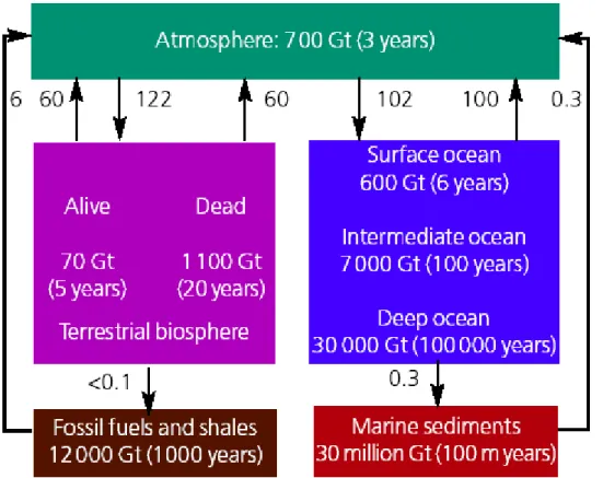
Figure 1.1 shows the major carbon reservoirs and the rates at which carbon is transferred
among these reservoirs, known as the carbon cycle. Two features are immediately evident: i) the water column of the oceans holds much more carbon than the atmosphere, although much lower than in marine sediments; ii) the exchange between the atmosphere and the biosphere and between the atmosphere and the surface oceans is much higher than the other fluxes. Looking at the relative sizes of the reservoirs of carbon, it might at first sight surprising that the burning of fossil fuels could be a problem because there appears to be plenty of capacity for the uptake of CO2 from the atmosphere into other reservoirs, especially the oceans.
One of the more commonly known exchanges in the carbon cycle is its absorption, in the form of CO2 by trees and herbaceous plants on land during photosynthesis (the production of
organic carbon from inorganic carbon), and subsequent release back into the atmosphere by respiration. As shown on Figure 1.1, every year the atmosphere exchanges ∼122 PgC (1 Pg = 1Gt = 1015 g) with the terrestrial ecosystems through photosynthesis and respiration. The uptake of carbon through photosynthesis is gross primary production (GPP). At least half of this production is respired by the plants themselves (autotrophic respiration), leaving a net primary production (NPP) of ∼60 PgC. Recent estimates of global terrestrial NPP vary
between 56.4 and 62.6 PgC yr-1 (Houghton, 2005). NPP is largely consumed by grazers such as insects and various kinds of animals or decomposed by fungi and bacteria. Live biomass is estimated to be about 550 PgC mainly in the form of wood (Houghton, 2005).
Figure 1.1: Diagram of the global carbon cycle showing sizes of carbon reservoirs (units are gigatonnes (Gt);
(1Gt = 1015 grams) and exchanges rates (fluxes) between reservoirs (units are Gt yr-1) in the terrestrial (green)
and the oceanic (dark blue) parts of the Earth system. Also shown are residence times (in years) of carbon in each reservoir: however, some mixing between the deep oceans and marine sediments does occur on shorter timescales. Carbon exchanges readily between the atmosphere, the surface oceans and terrestrial biosphere. However, the residence time of carbon in the atmosphere, oceans and biosphere combined, relative to exchange with the solid earth, is about 100 000 years (Royal Society, 2005). Note that this budget does not take account the CO2 fluxes in coastal ecosystems, continental aquatics ecosystems and the continental weathering.
After death it turns to litter and eventually to soil organic matter. Deforestation reduces the uptake of atmospheric CO2 by terrestrial biosphere and on the long term, this will
be an additional source of CO2 to the atmosphere at the rate of about 1 to 2 PgC yr-1
(Goudriaan, 1995). However, satellite observations and model estimates indicate that the global NPP of land ecosystems has increased by 6% (3.4 PgC between 1982 to 1999) (Nemani et al., 2003). The largest increase was in tropical ecosystems particularly in the
Amazon region. Despite this fact, tropical regions are not, on average, a significant net sink for carbon due to the fact that at such latitudes, NPP and soil respiration are tightly coupled compared with ecosystems at other latitudes. Thus, in the future, the combined effects of higher CO2 concentrations, warmer temperatures and changing hydrological regime will
significant affect regional ecology processes and hence carbon dynamics (Nemani et al., 2003). 4 5 6 7 8 9 10 11 0 500 1000 1500 2000 2500 CO2 HCO3 -CO3 2-Range of seawater pH C o n cen tr at io n s ( µm o l k g -1)
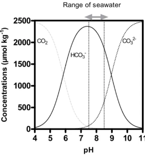
Figure 1.2: Variation of the concentrations (µmol kg-1) of the three inorganic forms of CO2 dissolved in
seawater as function of pH. The arrows at the top indicate the narrow range of pH (7.5-8.5) that is likely to be found in the oceans now and in the future.
Carbon dioxide also dissolves in the oceans and can be released back to the atmosphere, making the oceans a considerable point of exchange in the carbon cycle. Dissolved CO2 in seawater exists in three main forms collectively known as dissolved
inorganic carbon (DIC): i) aqueous CO2 (about 1% of DIC); in the present thesis this term
also includes carbonic acid (H2CO3); ii) bicarbonate ion (HCO3-, about 90% of DIC); and iii)
carbonates ion (CO32-, about 9% of DIC). Thus under current ocean conditions (pH between
7.5 and 8.5), bicarbonate is the most abundant form of DIC in seawater followed by carbonate and aqueous CO2 (Figure 1.2). One of the overall effects of CO2 dissolving in seawater is to
increase the concentrations of hydrogen ions (H+). This is the result of an initial reaction between water (H2O) and CO2 to form H2CO3. This weak acid readily releases H+ and is in
equilibrium with CO32- and HCO3- and as shown on Figure 1.2, the concentration of the three
forms of DIC is a function of the pH of seawater. Thus DIC operates as a natural buffer to the addition of H+ and it is called the seawater carbonate buffer. However, the capacity of the
buffer to restrict pH ranges diminishes as increased amounts of CO2 are absorbed by oceans.
This is because when CO2 dissolves, the thermodynamic equilibrium that take place reduces
the amount of CO32- ions, which are required for the seawater buffer. Based on recent
measurements in the North Sea, Thomas et al. (2007) demonstrate a significant decline in the buffering capacity in the inorganic carbonate system in the surface waters due to the uptake of anthropogenic CO2. The projections of future pH change also show that if the release of CO2
from human activities is allowed to continue on present trends this will lead to a decrease in pH of up to 0.5 units by the year 2100 in the surface oceans (Caldeira and Wickett, 2005).
Lower surface water temperatures tend to increase CO2 uptake, whilst surface
warming drives its release (e.g., Hales et al., 2003). This process is known as the solubility pump and it is quite efficient in atmospheric CO2 uptake at high latitudes. Warming of the
oceans leads to increased vertical stratification, which would reduce CO2 uptake, in effect,
reducing the oceanic volume available to CO2 absorption from the atmosphere. Stratification
will reduce the return flow of both carbon and nutrients from the depth to the surface. The removal of nutrients from the upper oceans with a slower return flow could have negative impact on life in the surface oceans. In fact, organisms within the surface ocean exchange CO2 in much the same way as the biological processes on land. Although the biological
uptake (also called the biological pump) of CO2 per unit area of the surface ocean is lower
than that in the most terrestrial systems, the overall biological absorption is almost as large as that in terrestrial environment due to the fact that oceans occupy 70% of the Earth’s surface (Field et al., 1998). Without the biological pump, the upper oceans would be oversaturated with respect to CO2 and the atmospheric levels of CO2. This biological pump can be separated
into an organic pump and calcium carbonate pump. The gross flux of organic pump is estimated to be 20-51 PgC yr-1 (Wong and Matear, 1995). The calcium carbonate (CaCO3)
pump plays also an important role in the marine carbon cycle. In the upper ocean, several autotrophs and heterotrophs form calcium carbonate skeletons by precipitating carbonate ions. The biogenic CaCO3 particles can sediment to depth (CaCO3 pump) where they can dissolve
or be preserved in sediments. The calcium CaCO3 pump creates a surface depletion of DIC
and alkalinity (TA) as described by the following equation:
Although the CaCO3 pump exports carbon the increase of CO2 in surface waters creates a
source for atmospheric CO2.
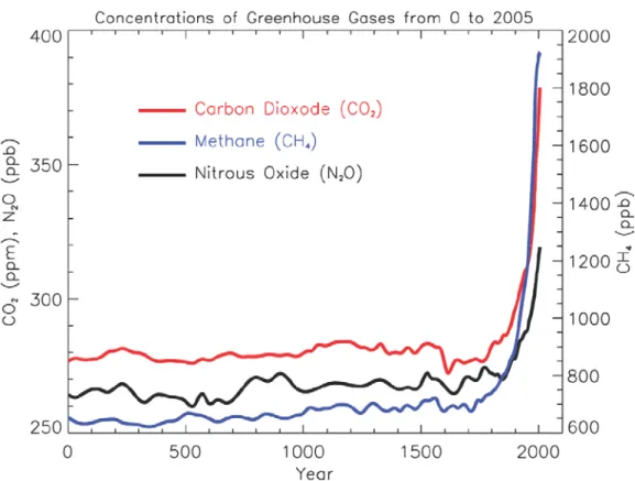
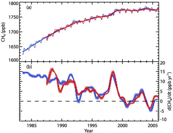
Figure 1.3: Atmospheric concentrations of important long-lived greenhouse gases over the last 2000 years.
Increases since about 1750 are attributed to human activities during the industrial era. Concentration units are parts per million (ppm) or parts per billion (ppb), indicating the number of molecules of the greenhouse gas per million or billion air molecules, respectively, in an atmospheric sample (IPCC, 2007).
The oceans are a substantial carbon reservoir (Figure 1.1) and on short timescales (~ 100 yr), the largest CO2 fluxes are with the atmosphere. The pre-industrial oceanic carbon
reservoir has been estimated at about 38 000 PgC, compared with the about 700 PgC in the atmosphere and somewhat less than 2000 PgC in the terrestrial biosphere (Brovkin et al., 2002). These reservoirs exchange quantities of carbon each year that are large relative to the amount of carbon stored within the reservoirs themselves. Figure 1.1 shows that the oceans are acting as an important carbon sink, absorbing 2 PgC yr-1 more CO2 than they are releasing
into the atmosphere. This is small in comparison to the amount of carbon that is cycled between the different reservoirs but is a significant proportion of the 6 GtC yr-1 into the atmosphere from human activities (Figure 1.1). However, it is important to note that, in this
budget neither the fluxes of CO2 in the coastal ocean nor in the freshwater ecosystems are
taken account. As it will be discussed in the next sections, coastal environments are very heterogeneous and they are characterised by high spatial and temporal variability of surface partial pressure of CO2 (pCO2). Some are sources of CO2 to atmosphere while the others are
acting as sinks of atmospheric CO2. Because of this variability, it is difficult to integrate the
corresponding fluxes in the global budget. Freshwater ecosystems (streams, lakes, reservoirs, wetland and rivers) are sources of CO2 to the atmosphere but, they are generally neglected in
the global budget. Continental weathering acts as a sink of atmospheric CO2 and could
represent a flux of about 0.7 PgC yr-1 of carbon exported from the continent to the oceans (Ludwig et al., 1998). Thus, the inclusion of CO2 fluxes from continental ecosystems and the
coastal ecosystems could reduce the gap estimates of the terrestrial carbon sink based on the carbon-stock change models globally (Siemens, 2003) or regionally (Borges et al., 2006).
The carbon stored in some reservoirs, such as rocks and organic rich shale, exchanges with the other reservoirs on geological timescales. As a result, these reservoirs will not affect the carbon content of the atmosphere or the oceans on shorter timescales (<1000 years) unless exchange rates are artificially increased by human activities such as limestone mining, oil, gas and coal extraction and consumption. It is well established today that human activities have increased atmospheric concentrations of CO2 to levels unprecedented for at least 420 000
years and possibly for the past tens of millions of years (IPCC, 2007). Antarctica ice core data indicate that atmospheric CO2 concentrations during the past 650 000 years are highly
correlated with changes in temperatures, varying between minima of ∼200 parts per million (ppm) during cold glacial periods and maxima of 280 to 300 ppm during interglacials. By comparison, atmospheric concentrations of CO2 averaged 380 ppm in 2005 (IPCC, 2007).
Prior to industrial revolution, land use change was likely a human source of greenhouse gas (GHG) emissions. The land clearing and rice cultivation by expanding human settlements in Europe and Asia (during the late Holocene) already began to alter the atmospheric composition of greenhouse gases, thus making the onset of the “Anthropocene era” of earth climate history (Ruddiman, 2003). Figure 1.3 shows the atmospheric concentrations of the most important natural occurring greenhouse gases (besides water vapour) over the last 2000 years (IPCC, 2007). Increases of greenhouse gases since about 1750 are attributed to human activities during the industrial era. Currently CO2 accounts for ~63% of anthropogenic
to CO2 (Table 1.1), CH4 and N2O currently contribute ~18% and ~6%, respectively, to
anthropogenic greenhouse forcing (IPCC, 2007).
Table 1.1: Global warming potentials (GWP) of CO2, CH4 and N2O (CO2-equivalent*); estimates for 20, 100,
and 500 year timeframes (Upstill-Goddard et al., 2007).
20 years 100 years 500 years
CO2 1 1 1
CH4 62 23 7
N2O 275 296 156
*CO2-equivalent emission is the amount of CO2 that would cause the same time-integrated
radiative forcing over a given time horizon, as an emitted amount of a long-live greenhouse gas (GHG) or a mixture of greenhouse gases (GHGs). The equivalent CO2 emission is
obtained by multiplying the emission of a GHG by its GWP for the given time horizon. For a mix of GHGs, it is obtained by summing the equivalent CO2 emissions of each gas.
Equivalent CO2 emission is a standard and useful metric for comparing emissions of different
GHGs but does not imply the same climate change responses (IPCC, 2007).
Roughly half of the CO2 released by human activities between 1800 and 1994 is now
stored in the ocean (Sabine et al., 2004), and about 30% of modern CO2 emissions are taken
by oceans today (Feely et al., 2004). However, warming reduces terrestrial and ocean uptake of atmospheric CO2, increasing the fraction of anthropogenic emissions remaining in the
atmosphere (IPCC, 2007). In fact, whereas both land and ocean sinks continue to accumulate carbon on average at 5.0 ± 0.6 PgC yr-1 since 2000; large sinks have been weakening
(Canadell et al., 2007). For instance, in the Southern Ocean, the poleward displacement and intensification of westerly winds caused by human activities (related to both greenhouse gas emissions and ozone loss) has enhanced the ventilation of carbon-rich waters normally isolated from the atmosphere at least since 1980, and contributed nearly half of the decrease in the ocean CO2 uptake (Le Quéré et al., 2007). On land, a number of major droughts in mid
latitude regions in 2002-2005 have contributed to the weakening of the growth rate of terrestrial carbon sink in these regions (Canadell et al., 2007). Continued uptake of
atmospheric CO2 is expected to substantial decrease oceanic pH over the next few centuries,
changing the saturation horizons of aragonite, calcite and other minerals essential to calcifying organisms (Kleypas et al., 1999; Feely et al., 2004; Orr et al. 2005).
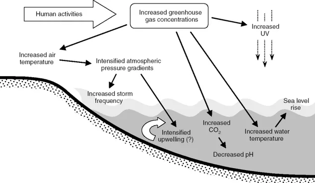
Figure 1.4: Important abiotic changes associated to climate change (Harley et al., 2006). Human activities such
as fossil fuel burning and deforestation lead to higher concentrations of greenhouse gases in the atmosphere, which in turn leads to suite of physical and chemical changes in coastal oceans. The question mark indicates that the relationship between climate change and upwelling is uncertain.
While many organisms have adapted to thermal fluctuations in the last few millions years, the expected change in pH are higher than any other pH changes inferred from the fossil record over the past 200-300 millions years (Caldeira and Wickett, 2003). Together, elevated atmospheric CO2 and the resultant increase in the global mean temperature will result
in a cascade of the physical and chemical changes in marine systems (Figure 1.4). Because warming trends will be stronger over continental interiors than over oceans, the atmospheric pressure gradient, and thus wind fields, along the ocean margins will intensify (Harley et al., 2006). Atmospheric circulation changes might also change storms frequency (Bromirski et al., 2003), and will also influence precipitation patterns that will affect coastal salinity, turbidity and inputs of terrestrial-derived nutrients and pollutants (IPCC, 2007). Climate change could
also alter large scale ocean circulation. Increasing CO2 levels in the atmosphere have been
postulated to deplete the ozone layer (Austin et al., 1992), potentially leading to enhanced levels of ultraviolet radiation at the Earth’s surface.
1.1.2 Air-water CO2 exchanges:
The sequestration of atmospheric CO2 by the surface water depends on differences in
the partial pressure of CO2 between the surface water (pCO2water) and the atmosphere (pCO2 air), ∆pCO2. When ∆pCO2 is positive, i.e. pCO2 water is greater than pCO2air, CO2 gas escapes
from the surface water to the atmosphere; the aquatic ecosystem is referred as a source of CO2. If ∆pCO2 is negative then the aquatic ecosystem is a sink for atmospheric CO2. The
magnitude of the air-sea flux of CO2 (F in mmol m-2 d-1) between the surface water and
atmosphere is described by the following equation:
F= ε.α.k.∆pCO2 (2)
The flux is a function of the chemical enhancement factor of gas exchange (ε; that is usually negligible, except under very low turbulent conditions), solubility coefficient (α in mol atm-1 m-3), gas transfer velocity (k in cm h-1) and ∆pCO2 (in ppm).
Methodology for measuring pCO2 in both air and water has progressed to the stage
where it is now possible to make continuous, accurate measurements of the ∆pCO2 by a
variety of means in almost any type of aquatic system. Thus, the largest uncertainty in the computation of F comes from k (since α is straightforwardly computed from salinity and water temperature) that depends on water turbulence mainly generated by wind stress and on a number of processes including surfactant damping, boundary layer stability, precipitation, air bubbles, wave breaking and evaporation/condensation. Therefore, developing accurate estimates of the gas transfer velocity in aquatic systems is an important and controversial research (e.g., Raymond and Cole, 2001; Borges et al., 2004). For consistency, k is often reported as k600 or k660 which is k for CO2 at 20 °C (Schmidt number, (Sc)) of 600 or 660 in
freshwater and seawater, respectively. The Schmidt number is defined as the ratio of transfer coefficients for momentum and mass, which are respectively kinematic viscosity of water (νw
is specific to a given gas, and depends on temperature and salinity and is related to the Schmidt number by the following equation:
Sc = νw/D (3)
Thus, the main resistance to the CO2 transfer across the air-water interface is due to
molecular diffusion through a laminar layer of water adjacent to the air-water interface. The thickness of this layer (~10 to ~100 µm) controls k and depends largely on the wind speeds in open oceans, while in rivers and streams, the source of turbulence is mainly due to bottom stress of the flow and k is a function of the stream depth and flow velocity. In estuaries, turbulence in water can originate from both wind and tidal currents, and therefore depends on the depth, mean tidal velocity, and wind regime of a given estuary. For instance, Borges et al. (2004) showed that the contribution of turbulence generated by tidal current is negligible in the microtidal estuary (such as Randers Fjord) while is significant at low to moderate wind speeds in macrotidal estuaries (such as Scheldt and Thames).
The way turbulence is taken account results in three main models of gas transfer at water surfaces (Brtko and Kabel, 1978). These models differ in the way the molecular diffusivity coefficient is accounted, hence also the Schmidt number.
In the film model, it is postulated that adjacent to the free liquid surface there exists a stagnant film below which the liquid is well mixed. It assumed that air-water exchange of gas is mainly controlled by molecular diffusion in the boundary layer (film). The film represents then the major resistance to the air-water exchange. The gas transfer velocity is therefore proportional to molecular diffusion:
k ∝ D ∝ Sc-1
The boundary layer model was first developed for smooth and rigid surfaces and then adapted for rough surfaces. In this model the mass transfer process is characterized by molecular diffusion into fluid elements transported from the bulk liquid to near the free liquid surface by turbulent eddies. The diffusion of mass into the fluid elements occurs for a prescribed time which is assumed to be uniform for all turbulent eddies. According this model
k is given by: k ∝ D2/3 ∝ Sc-2/3
The surface renewal model considers that there should be a random age distribution of fluid elements rather than a uniform contact time. The fractional rate of replacement of the fluid elements belonging to any age group is assumed to be equal to the surface renewal rate. The air-water exchange is then limited by the rate of replacement of the micro-layer and k is given by:
k ∝ D0.5 ∝ Sc-0.5
However, on the whole, wind speed is recognised as the main factor on k, since the effects of other factors such as waves, air bubbles, surface films, heat exchange at the interface are more or less directly related to wind conditions. Therefore, a variety of different parameterizations of k as a function of wind speed were proposed to calculate the CO2 transfer
velocity based on fields (deliberate tracers SF6 and 3He, bomb produced 14C, 222Rn deficiency
method, floating bell method, eddy covariance, gradient flux technique) or laboratory approaches (wind-tunnel experiments). Simple linear relationships were suggested by Smethie et al (1985) and Tans et al. (1990), whereas Liss and Merlivat (1986) described k by three separated linear functions that each refer to different states of the sea surface. Functions including a quadratic term were proposed by Wanninkhof (1992), Jacobs et al. (1999), Nightingale et al. (2000) and Ho et al. (2006) whereas cubic functions have been considered by Schneider et al. (1999) and Wanninkhof and McGillis (1999). The most frequently k-wind relationships used in the open ocean are those from Liss and Merlivat (1986), Wanninkhof (1992), Wanninkhof and McGillis (1999) and Nightingale et al. (2000).
In estuaries, four approaches can be used to obtain k: natural tracers, purposeful tracer additions, floating domes and micro-meteorological methods (eddy covariance and gradient flux technique). However, k values obtained through these approaches are fairly different particularly at high wind speeds. Raymond and Cole (2001) argued that only the natural tracer approach provides the correct estimates of k in estuaries. However, Borges et al. (2004) based on floating method in three European estuaries, showed that the formulation of k as a function of wind speed is site specific in estuarine environments. Thus, there is no consensus hitherto to choice the best k formulation in estuarine environments and future works will help to resolve gas transfer velocity in these ecosystems. In the present work, only the formulations of k as function of wind speed from Carini et al. (1996) and Raymond and Cole (2001) have been used. These two k formulations as a function of wind speed are based on natural and
deliberate tracers and values computed can be considered conservative (Zappa et al., 2003; Borges et al., 2004; Zappa et al. 2007).
Air-water exchange processes of CO2 are much slower compared to other processes
such as biological activity or even temperature change. Furthermore, due to seawater buffer effect, only a larger amount of CO2 needs to be transferred to restore the equilibrium between
the atmosphere and water surface than in freshwater. This buffering effect of seawater is called the Revelle factor (β). It is the ratio of the fractional change of pCO2 in the water to the
fractional change of the DIC in the water. This is an important quantity because it allows predicting the capacity of surface water to take up the anthropogenic atmospheric CO2.
β = (∆pCO2/pCO2)/( ∆DIC/DIC) (4)
β is about 14 for cold waters and 8 for warm waters (the global ocean average value is about 10). Thus, a 10% change in pCO2 only results in a 1% DIC and air-water CO2 exchange
have a small effect on the DIC dynamics in water column.
Based on the air-water CO2 fluxes, the world oceans can be divided into 3 major areas:
i) CO2 source areas in the equatorial oceans (mainly the equatorial Pacific) and in the coastal
upwelling zones caused by the supply of CO2 rich deep water, e.g. along the east boundary
currents (California current, Humboldt current, Benguela current, …); ii) CO2 sink areas in
both hemispheres where enhanced solubility of CO2 in the surface waters makes these areas
capable of absorbing CO2 from the atmosphere, e.g. the Sargasso sea in North Atlantic where
high evaporation over precipitation produces very alkaline waters, or the Labrador sea and Weddell sea where cold surface water has high CO2 solubility; iii) seasonal CO2 source/sink
areas where a complex interplay occurs between CO2 uptake created by high productivity in
summer and the high CO2 solubility in winter and CO2 release by winter remineralisation of
1.1.3 CO2 chemistry in natural waters
The following section is based on DOE (1994), Millero (2007) and Dickson et al. (2007). CO2 in the atmosphere is a chemically uncreative gas but, when dissolved in water it
reacts through thermodynamic equilibrium with bicarbonate (HCO3-), carbonate (CO32-) and
hydrogen (H+) ions. The CO2 chemistry in water is intimately linked to pH (Figure 1.2)
according to the following equations:
CO2 (g) ←→CO2 (aq) (5)
CO2 (aq) + H2O (1) ←→ H2CO3 (aq) (6)
H2CO3 (aq) ←→ H+(aq) + HCO3- (aq) (7)
HCO3- (aq) ←→ H+ (aq) + CO32- (8)
The notations (g) and (aq) in equation (5) refer to the state of CO2, respectively in gaseous
and dissolved in seawater. It is not possible to analytically distinguish between the species CO2 (aq) and H2CO3 (aq) and the latter is present in small quantities ([CO2 (aq)]/([H2CO3
(aq)] ∼ 650). Thus, these species are combined as the sum of the concentration of a hypothetical species, CO2* (aq).
CO2* (aq) = CO2 (aq) + H2CO3 (aq) ≈ CO2 (aq) (9)
Redefining (5), (6) and (7), one gets: CO2 (g) ←→ CO2* (aq) (10)
CO2* (aq) + H2O (1) ←→ H+ (aq) + HCO3- (aq) (11)
The equilibrium constant of equations (8) and (11) are given by: K1 = [H+] [HCO3-]/ [ CO2*] (12)
K2 = [H+] [CO32-]/[HCO3-] (13)
While the pCO2 is related to [CO2*] by Henry’s law:
K0 = [ CO2* ]/pCO2 (14)
K0 is the solubility coefficient of CO2 (µmol kg-1 µatm-1) and K1 and K2 are the first and
second dissociation constants of carbonic acid, respectively. These equilibrium constants above are dependant on temperature, pressure and salinity of the solution (e.g., seawater). Note that strictly, equations (12) to (13) should be expressed in terms of activities rather than concentrations. However, it is not possible analytically to determine activities of HCO3-,
CO32- or CO2 since the concentration of a single ion cannot vary independently since
electroneutrality is required. Hence, ocean chemists use apparent thermodynamic constants to examine the carbonate system. Furthermore, as the activity coefficients are approximately constant for the small amounts of reacting species in a background medium, these expressions are valid and correspond to “ionic medium” equilibrium constants based on a seawater medium.
The term pH describes the acidity of the medium and is defined as:
pH = -log(aH+) (15)
Where aH+ is the activity of H+
It is measured using a combined electrode or by spectrophotometry (in the present work a combined electrode method was used). However, as notice above, it is not possible to determine individual activities of ions. To overcome this situation, four operational definitions of pH in water were proposed. The first practical definition of pH (also called NBS scale) was given by the U. S. National Bureau of Standards. The pHNBS of a solution
determined from measurements the electrode potential (mV) is given by the following equation
:
Where pH (X) and pH (S) are respectively the pH of water sample and the standard (buffer) at a given temperature, E (S) and E (X) are respectively the electrode potential (mV) of the standard and the sample water, R is the gas constant (8.3145107 J K-1 mol-1), T is the
absolute temperature (K), and F is the Faraday constant (96485.30929 °C mol-1).
In solutions of high ionic strength, this scale does not give reliable values due to differences in liquid junction potentials of combined electrodes in the dilute buffers and the ionic media. Thus, it not recommended for seawater pH measurements, but it is appropriate for pH measurements in freshwater and brackish waters, such as estuaries, lagoons and mangrove ecosystems (Frankignoulle and Borges, 2001b). The three other pH scales have been developed for seawater based on the use of buffers made from artificial seawater, that largely overcome the problem of junction potential, since buffers and samples have similar ionic strengths. The difference between these three pH scales relies on the fact that the protons in seawater interact with sulphate and fluoride ions. The definition of these three pH scales is given in Table 1.2:
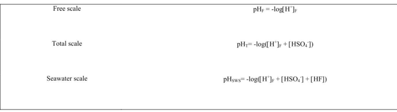
Table 1.2: Definition of pH scales in seawater
Free scale pHF = -log[H+]F
Total scale pHT= -log([H+]F + [HSO4-])
Seawater scale pHSWS= -log([H+]F + [HSO4-] + [HF])
Note that in practice, the pH of seawater samples is computed using the Nernst equation given by equation (16). According to Dickson (1993), the Free scale is inappropriate because it omits the interaction with sulphate and fluoride ions, thus inducing an important bias in the pH measurements. The difference of pH measured on the Total hydrogen ion concentration scale and Seawater scale is very low (0.001), since [HSO4-] is much higher than [HF] in
seawater. Therefore, the Total hydrogen ion concentration is the most appropriate and commonly used pH scale for seawater samples.
One of the fundamental approach in inorganic carbon chemistry is the determination of the speciation, i.e. the concentrations of H+, CO
2*, HCO3- and CO32-. Assuming that the values of
K1 and K2 are known (determined from empirical formulations as a function of salinity and
temperature), equations 12 and 13 constitute a system of two equations with four unknowns. Two additional equations that do not introduce additional unknowns are then needed to solve the speciation. There are four parameters that can be measured: pH, TA, DIC, and pCO2. A
combination of two of these parameters is used together K1 and K2 to obtain the speciation of
the carbon dioxide system in water.
DIC is the sum of the three dissolved inorganic carbon species:
DIC = [CO2*] + [HCO3-] + [CO32-] (17)
The relative contribution to DIC of each species for standard seawater is approximately 90, 9 and 1% from respectively HCO3-, CO32- and CO2*. Thus, CO2* that is involved in
air-seawater exchange and photosynthesis and respiration is a minor part of DIC. Also, CO3
2-involved in calcification and CaCO3 dissolution is also in much lower concentrations than
HCO32-. In freshwater ecosystems (e.g., rivers, lakes), the contribution of CO2* to DIC pool is
also low where HCO3- account for more than 80% of DIC.
The currently accepted definition of TA was proposed by Dickson (1981): the number of moles of hydrogen ion equivalent to the excess of proton acceptors (bases formed from weak acids with dissociation constant K ≤ 10-4.5 at 25°C and zero ionic strength) over proton donors
(acids with K > 10-4.5) in 1 kilogram of sample. TA is given by the following equation:
TA = [HCO3-] + 2[CO3-2] +[B(OH)4-] + [OH-] + [HPO42-] + 2[PO43-] + [SiO(OH)3-] +
[NH3] + [HS-] + 2[S2-] - [H+] - [HSO4-] - [HF] - [H3PO4] (18)
TA relates readily to the titration of water with a strong acid, usually HCl, in which the equivalence point is determined by following the decrease of pH. TA is therefore sometimes referred as titration alkalinity. In common seawater conditions, most species can be neglected
in comparison with the bicarbonate and carbonate concentrations, except for borate so the above equation can be rewritten as follows:
TA = [HCO3-] + 2[CO3-2] +[B(OH)4-] + [OH-] - [H+] (19)
The other components are minor species. However, in anoxic environments (such as estuaries), polluted rivers, or in phosphate and silicates rich deep seawater samples, the contribution of minor species can be significant. The borate ion does not introduce an additional unknown in the inorganic carbon calculations because its concentration can be readily computed from salinity, temperature and pH according the following equations:
B(OH)3 + H2O ←→ B(OH)4- + H+ (20)
KB = [B(OH)4-].[H+]/[B(OH)3] (21)
BT = [B(OH)3 ] + [B(OH)4-] (22)
[B(OH)4-] = KB.BT/([H+]+BT) (23)
BT is computed as a function of salinity.
Carbonate alkalinity (CA) is given by the following equation:
CA = [HCO3-] + 2[CO3-2] (24)
Equation 19 can be rewritten as:
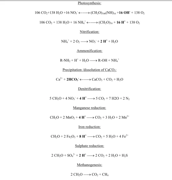
In the open ocean TA is conservative with salinity (e.g., Millero et al., 1998) but in coastal environments TA can be affected by several aerobic/anaerobic reactions that produce or consume protons (Table 1.3). During photosynthesis, TA increases due to the consumption of nitrates whereas the assimilation of ammonium has an opposite effect. The consumption of CO2 during photosynthesis decreases DIC, pCO2 and increases pH, whereas the aerobic
respiration will obviously have the opposite effect of photosynthesis on DIC, pCO2 and pH.
Ammonification increases TA (proton consumption), whereas nitrification decreases TA (proton production).
Denitrification, Maganese, Iron and sulphate reductions, and methanogenesis that are anaerobic organic carbon degradation processes release CO2 and therefore increase DIC,
pCO2 and decrease pH. All these processes (except the methanogenesis) increase TA by the
consumption of protons. Anoxic processes occur mainly in the sediments, and due to the much larger abundance in seawater of SO42-, sulphate reduction is the main anaerobic
diagenetic organic matter degradation pathway. In presence of O2, H2S is oxidized producing
protons.
Hence, a net flux of TA from the sediment to the water column should not occur unless reduced sulphur is permanently trapped, namely as pyrite, which only significantly occurs in iron rich sediments such as those of mangrove ecosystems. Furthermore, the acidification related to the production of protons from the oxidation of H2S in sub-oxic and oxic layers of
the sediments can lead to the dissolution of calcium carbonate (CaCO3) and a net TA
Table 1.3: stoichiometry of reactions that can affect TA, DIC, pCO2 and pH in aquatic environments (adapted from Abril and Frankignoulle, 2001). R represents organic mater.
Photosynthesis: 106 CO2+138 H2O +16 NO3- ←→ (CH2O)106(NH)16 +16 OH- + 138 O2 106 CO2 + 138 H2O + 16 NH4+ ←→ (CH2O)16 + 16 H+ + 138 O2 Nitrification: NH4+ + 2 O2 → NO3- + 2 H+ + H2O Ammonification: R-NH2 + H+ + H2O → R-OH + NH4+
Precipitation /dissolution of CaCO3:
Ca2+ + 2HCO 3- ←→ CaCO3 + CO2 + H2O Denitrification: 5 CH2O + 4 NO3- + 4 H+ → 5 CO2 + 7 H2O + 2 N2 Manganese reduction: CH2O + 2 MnO2 + 4 H+ → CO2 + 3 H2O + 2 Mn2+ Iron reduction: CH2O + 2 Fe2O3 + 8 H+ → CO2 + 5 H2O + 4 Fe2+ Sulphate reduction: 2 CH2O + SO42- + 2 H+ → 2 CO2 + 2 H2O + H2S Methanogenesis: 2 CH2O → CO2 + CH4
Calcification also affects TA and DIC dynamics. Calcification is the biologically mediated precipitation of CaCO3 by either planktonic (coccolithophores, foraminifera,
pteropods, …) or benthic (bivalves, corals, calcareous algae, …) organisms. Carbonate minerals are present in various forms such as calcite, aragonite and mixed calcium/magnesium carbonates. Calcite and aragonite are both calcium carbonate forms and they differ in their crystallographic structure. The precipitation of CaCO3 is given by equation
(1). For each mole of CaCO3 precipitated, one mole of CO2 is released. However, the released
CO2 will interact with HCO3- and CO32- by thermodynamic equilibria, hence the ratio (ψ) of
and in particular on temperature. In freshwater ψ = 1 and for standard seawater conditions ψ = 0.6. Calcification decreases DIC but the resulting production of CO2 can lead to
oversaturation of CO2 with respect to the atmospheric content as shown in coral reefs (e.g.
Gattuso et al., 1993, 1996; Frankignoulle et al., 1996). In the open ocean, the most important pelagic calcifying organisms are coccolithophorids. Purdie and Finch (1994) and Crawford and Purdie (1997) have shown that coccolithophorid calcification was a source of CO2 to the
water mass and a potential source to the atmosphere, when the release of CO2 exceeds its
consumption (e.g. Head et al., 1998). The effect of calcification on carbonate speciation reduced the air-sea pCO2 gradient by ~15 ppm in a huge coccolithophorid bloom in the North
Atlantic (Robertson et al., 1994). Bates et al. (1996) reported TA depletion in the upper water column of the Sargasso Sea was associated to higher pCO2 values and were probably the
biogeochemical signature of calcification. In the Bering Sea, TA decreases of more than 80 µmol kg-1 have been reported in association with coccolithophore blooms (Murata and Takizawa, 2002). In the Bay of Biscay, decreases of TA of ~30 µmol kg-1 lead to an increase of surface water pCO2 values of about 50 ppm, yet did not induce an over-saturation of CO2
and the area still acted as a sink for atmospheric CO2 (Borges, unpublished; Suykens et al.,
2008).
The degree of saturation of seawater with respect to aragonite or calcite (Ωarg or Ωcal)
is the ion product of the concentrations of calcium and carbonate ions divided by the stoichiometric solubility product (Ks), at the in situ temperature, salinity, and pressure:
Ωarg = [Ca2+] [CO32-]/Ksarg. (26)
Ωcal = [Ca2+] [CO32-]/Kscal. (27)
Where the calcium concentration is estimated from salinity and the carbonate ion concentration is calculated from the DIC and TA data. Because the ratio calcium to salinity in seawater does not vary by more than 1.5%, variations in the ratio of [CO32-] to the
stoichiometric solubility product primarily govern the degree of saturation of seawater with respect to aragonite and calcite.
Ωarg (Ωcal)> 1 corresponds to aragonite (calcite) oversaturation, when CaCO3 precipitation
is thermodynamically favoured and Ωarg (Ωcal)<1 correspond to aragonite (calcite)
under-saturation when CaCO3 dissolution is thermodynamically favoured.
Until recently, it had been commonly though that the dissolution of pelagic CaCO3
particles primarily occurs below the calcite saturation depth (Ωcal =1). However, recent
analyses of the global carbonate budget and carbonate data for the global oceans have indicated that perhaps as much as 60 to 80% of the CaCO3 that is exported out of the surface
ocean dissolves in the upper 1000 m (Feely et al., 2004). Milliman et al. (1999) explored the biologically mediated dissolution above the saturation horizon and suggested various pathways by which dissolution could take place. Even if grazing pressure is supposed to contribute greatly to dissolution, the influence of microbial activity, whether it is associated or not within microenvironments, cannot be excluded.
Aragonite and magnesian calcite are at least 50% more soluble in seawater than calcite (Kawahata et al., 2000), suggesting that organisms that form these types of CaCO3 may be
particularly affected by ocean acidification (increasing pCO2 and decreasing pH in surface
waters leading to a decrease of CO32- and Ω).
The present day accumulation of CaCO3 in marine sediments is about 0.10 to 0.14 Pg
of CaCO3 per year along the continental margins or in deep sea, and 0.13 to 0.17 Pg of CaCO3
per year in continental shelf sediments (Catubig et al., 1998; Iglesias-Rodriguez et al., 2002). The global new production of CaCO3 ranges from 0.8 to 1.4 Pg of CaCO3 per year based on
models or observations of seasonal changes in alkalinity in the euphotic zone (Lee, 2001; Iglesias-Rodriguez et al., 2002). Balch et al. (2007) recently estimated global pelagic calcification to 1.6±0.3 Pg of CaCO3 yr-1, based on remote sensing data. Thus, of the total
amount of CaCO3 that is produced annually, no more than ~30% is buried in shallow and
deep sediments. The rest is dissolved in the water column, at the sediment-seawater interface or in the upper sediments (Feely et al., 2004).
1.1.4 CO2 dynamics in coastal zone and freshwater ecosystems 1.1.4.1 Carbon fluxes in rivers
Rivers, in particular, large rivers, play an essential role in the transport and transformation of carbon from the land and the atmosphere to the ocean (Sabine et al., 2003; Richey et al. 2002; Chen, 2004). Using an empirical model, Ludwig et al. (1998) estimated that a total of 0.721 PgC yr-1 is exported from the continents to the ocean. Of this total continental erosion flux, about 0.096 PgC yr-1 is as particulate inorganic carbon (PIC). Of the reaming 0.625 PgC, 33% is dissolved organic carbon (DOC), 30% as the particulate organic carbon (POC) and 37% as HCO3- from carbonate rock weathering. The total organic carbon
flux (0.394 PgC yr-1) to the ocean estimated by Ludwig et al. (1998) is similar to earlier estimates summarized by Smith and Hollibaugh (1993), although more recent literature has suggested fluxes between 0.43 and 0.50 Pg C yr-1 (Schlunz and Schneider, 2000; Mackenzie
et al., 2004). In a recent review, Richey (2004) argued that the POC flux alone can be as high as 0.50 PgC yr-1 if the higher sediment yield from tropical and subtropical mountainous rivers is included. The total riverine HCO3- flux of Ludwig et al. (1998) (0.329 Pg C yr-1) is
somewhat lower than that reported by Mackenzie and co-workers (0.41 Pg C yr-1; Mackenzie et al, 1998; Mackenzie et al., 2004). The flux of PIC has also been evaluated at higher rates of 0.180 Pg yr-1 (Mackenzie et al., 2004).
Nearly all carbon in the form of DOC and POC in rivers is directly or indirectly of atmospheric origin. Organic carbon flux (∼1.5 PgC yr-1) from land to the rivers carries the
biomass produced by photosynthesis (∼60 PgC yr-1) in excess of losses due to respiration and
forest fires (Schlesinger, 1997). During the transport towards the oceans, a large part of the organic carbon may be decomposed and released back to rivers and the atmosphere as CO2
through microbial respiration (Richey et al., 2002). Most of the terrestrial DOC and POC reaching the ocean are believed to be decomposed in the ocean margins with less than a total of 0.150 PgC yr-1 of POC being buried in marine sediments (Mckee, 2003). Most of inorganic carbon is transported as HCO3- and is derived from atmospheric CO2 involved in mineral
weathering and from the dissolution of carbonate minerals in sedimentary rocks. Consequently export rates from catchments will be strongly related to bedrock geology.
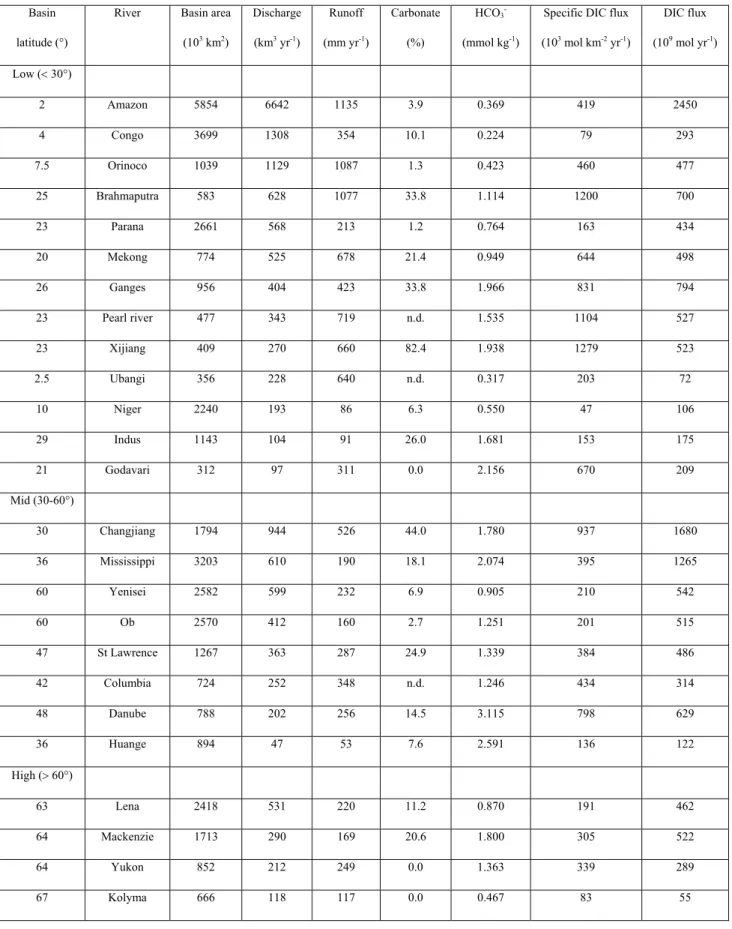
Table 1.4 gives the concentrations and fluxes of HCO3- in the 25 largest rivers in the world.
The following major features can be identified: i) HCO3- concentrations are highest in the mid
a low [HCO3-] of only 0.369 mmol kg-1 in contrast with the high average concentrations of
2.591, 1.780, 1.535 and 2.074 mmol kg-1 respectively in the Huange, Changjiang, Pearl and
Mississippi rivers; ii) Bicarbonate specific fluxes are highest in the mid latitude although the maximum shifts somewhat towards the subtropical rivers. The three mid latitude large rivers, the Changjiang, the Mississippi and the Columbia, have lower specific fluxes relative to the pattern of their concentrations, while the Huange has a very low specific HCO3- flux because
of low carbonate mineral content on the catchment and a dry climate; iii) As far as the total inorganic carbon flux is concerned, the three largest rivers that carry HCO3- to the oceans are
the Amazon, the Mississippi, and the Changjiang. These distribution patterns of HCO3
-concentration and flux are consistent with the global distribution pattern of continental carbonate rocks. For the 25 rivers, rivers in low (< 30°), mid (30-60°) and high (> 60°) latitudes have an average HCO3- concentration of 0.584, 1.649 and 1.154 mmol kg-1
respectively and they account for 43, 47 and 10% respectively of the total DIC flux to the ocean. Thus mid latitude rivers deliver a disproportionally high DIC flux with a relatively small (26%) amount of freshwater discharge (Cai et al., 2008). Mineral weathering is known to be a major regulator of atmospheric CO2 concentrations over geological time scales (Berner
et al., 1983). Recent studies of the Mississippi river HCO3- fluxes suggest that weathering
rates may change over much shorter time scales (e.g. over decades), and may respond to changes in land use (Cai, 2003; Raymond and Cole, 2003). This additional information highlights the pressing need for a better understanding of DIC export associated with weathering processes and temporal and spatial variations.
1.1.4.2 Processes controlling pCO2 in river waters
The pCO2 in river waters is controlled by both internal carbon dynamics and external
biogeochemical processes in upstream terrestrial ecosystems. These processes include: 1) production and transport of soil CO2; 2) in situ respiration and degradation of organic matter
within the water column; 3) photosynthesis by aquatic plants; 4) CO2 evasion from water to
air, in which the former two processes produce CO2 and make the water pCO2 increase, while
the latter two cause water pCO2 levels to decrease.
The surface pCO2 dynamics in river systems are closely related to the soils
mainly resulting from respiration and decomposition of organic matter, is generally much higher than ambient atmospheric CO2 (Finlay, 2003). The variation in soil CO2 content is
positively correlated with seasonal changes of temperature and precipitation in the basin (Jassal et al., 2004). When soils are wetted by precipitation, together with proper temperature and high retention times of waters in soils, active bacterial activities produce significant CO2
making soil become highly enriched in CO2 (Hope et al., 2004).
Dissolution of soil CO2 and subsequent transport to the stream via base flow and inter
flow is likely the main reason for pCO2 super-saturation in river waters. The seasonal
variation in soil CO2 content results in seasonal variation in pCO2 of river waters. In addition,
the intensity of rainfall, hydrological flow path and river discharge are other factors impacting pCO2 in river waters. Heavy rain that directly flows into the stream through surface runoff
without penetrating into the soil will dilute the pCO2 in river waters. Beside the dilution
effect, the fast flow velocity, which increases water turbulence, greatly enhances CO2
outgassing from river water to the atmosphere and it is another reason for lower pCO2 levels
during the flood periods. Biogenic CO2 uptake and release, i.e., photosynthesis of aquatic
plants and respiration and degradation of organic matter in the river itself also impact the pCO2 in river systems. In general, in situ photosynthesis takes up aqueous CO2, making the
water pCO2 decrease, while respiration and degradation of organic matter release CO2,
Table 1.4: Basic information and flux data for the 25 world’s largest rivers (Cai et al., 2008)
Basin latitude (°)
River Basin area (103 km2) Discharge (km3 yr-1) Runoff (mm yr-1) Carbonate (%) HCO3 -(mmol kg-1)
Specific DIC flux (103 mol km-2 yr-1) DIC flux (109 mol yr-1) Low (< 30°) 2 Amazon 5854 6642 1135 3.9 0.369 419 2450 4 Congo 3699 1308 354 10.1 0.224 79 293 7.5 Orinoco 1039 1129 1087 1.3 0.423 460 477 25 Brahmaputra 583 628 1077 33.8 1.114 1200 700 23 Parana 2661 568 213 1.2 0.764 163 434 20 Mekong 774 525 678 21.4 0.949 644 498 26 Ganges 956 404 423 33.8 1.966 831 794 23 Pearl river 477 343 719 n.d. 1.535 1104 527 23 Xijiang 409 270 660 82.4 1.938 1279 523 2.5 Ubangi 356 228 640 n.d. 0.317 203 72 10 Niger 2240 193 86 6.3 0.550 47 106 29 Indus 1143 104 91 26.0 1.681 153 175 21 Godavari 312 97 311 0.0 2.156 670 209 Mid (30-60°) 30 Changjiang 1794 944 526 44.0 1.780 937 1680 36 Mississippi 3203 610 190 18.1 2.074 395 1265 60 Yenisei 2582 599 232 6.9 0.905 210 542 60 Ob 2570 412 160 2.7 1.251 201 515 47 St Lawrence 1267 363 287 24.9 1.339 384 486 42 Columbia 724 252 348 n.d. 1.246 434 314 48 Danube 788 202 256 14.5 3.115 798 629 36 Huange 894 47 53 7.6 2.591 136 122 High (> 60°) 63 Lena 2418 531 220 11.2 0.870 191 462 64 Mackenzie 1713 290 169 20.6 1.800 305 522 64 Yukon 852 212 249 0.0 1.363 339 289 67 Kolyma 666 118 117 0.0 0.467 83 55
The active degree of biological activities in rivers is mainly controlled by seasonally and spatially changed temperature, turbulence and flow velocity of water. The pCO2 will change
seasonally or at different stretches because of changing biological activities. If biological activities are significant, biological CO2 uptake and release would cause great shifts in water
pCO2. Varying relative dominance of in situ respiration and degradation of organic matter
versus photosynthesis in different seasons and in different stretches makes pCO2 rise or fall.
In tropical rivers, the respiration and decomposition from floating and emerged macrophytes can constitute an important source of CO2 to the water column. For instance, in the Amazon
river root respiration from and decomposition of floating and emerged macrophytes contribute to 25% or more of CO2 evasion to atmosphere from the water column (Richey et al., 2002;
Engle et al., 2008).
Streams and rivers are usually net sources of CO2 to the atmosphere. For instance, CO2
evasion from global river systems extrapolated from mostly temperate rivers reaches about 0.3 PgC yr-1, nearly equivalent to riverine total organic carbon or DIC export (Cole and Caraco, 2001). Similarly, Richey et al. (2002) estimated that the loss of CO2 from rivers in
lowland humid tropical forests is 0.9 PgC yr-1. Such a large CO2 source urges us to reconsider
the global carbon budget, and direct measurements of land-atmosphere CO2 gas exchange that
ignore water-borne fluxes might significantly overestimate terrestrial carbon accumulation (Hope et al., 2001; Siemens, 2003; Borges et al., 2006). Therefore, CO2 degassing to the
atmosphere from river systems should be considered a significant component of regional net carbon budgets in future studies.
1.1.4.3 The role of freshwater ecosystems in the global carbon cycle
Figure 1.4 shows the role of inland aquatic systems in the global carbon balance.
Overall, freshwater ecosystems (particularly rivers, lakes, and reservoirs) receive 1.90 PgC yr
-1 from the terrestrial landscape of which 0.23 PgC yr-1 is buried in aquatic sediments, at least
0.75 (possibly much more) is returned to the atmosphere as gas exchange while the remaining 0.92 Pg C yr-1 is delivered to the oceans, roughly equally as inorganic and organic carbon (Cole et al., 2007). Thus, roughly twice as much carbon enters inland aquatic systems from land as is exported from land to the sea. In addition to transporting carbon to the oceans, freshwater systems represent an active component of the global carbon cycle that deserves