Proceedings ed. by M. Tisza
DEVELOPMENT OF AN INVERSE METHOD FOR IDENTIFICATION
OF MATERIALS PARAMETERS IN THE SINGLE POINT
INCREMENTAL FORMING PROCESS
C. Bouffioux1,a, C. Henrard2,b, Jun Gu1,c, J.R. Duflou3,d, A.-M. Habraken2,e, H. Sol1,f
1Vrije Universiteit Brussel, Department MeMC – TW Pleinlaan 2, 1050 Brussels, Belgium
e-mail: [email protected], [email protected], [email protected] Web page: http://www.vub.ac.be
2 Université de Liège, Department ArGEnCo – MS²F Chemin des Chevreuils 1, 4000 Liège, Belgium
e-mail: [email protected], [email protected] - Web page: http://www.ulg.ac.be 3 Katholieke Universiteit Leuven, Department PMA
Celestijnenlaan 300A, 3001 Heverlee, Belgium
e-mail: [email protected] - Web page: http://www.kuleuven.ac.be Key words: Inverse method, FEM simulation, incremental forming, sheet metal forming
Summary. The purpose of this article is to develop an inverse method for adjusting the
material parameters during single point incremental forming. The main idea consists in simulating tests performed on the same machine as the one used for the process itself. This reduces the costs of the equipment since no specific and costly standard test equipment is needed. Moreover, it has the advantage that the material parameters are fitted for a heterogeneous stress and strain state occurring during the real process. Before using the inverse method, the numerical results must be compared with the experimental ones. Several boundary conditions will be tested.
1. INTRODUCTION
Single Point Incremental Forming (SPIF) is a new sheet metal forming process adapted to both rapid prototyping and small batch production at low cost. A clamped sheet is deformed by a smooth-ended tool following a specific tool path defining the final required shape without specific and costly dies. A wide variety of shapes can be made [1, 2].
Accuracy of the F.E.M. simulations of this process depends both on the constitutive law chosen and the identification of the material parameters. The study of the process shows that the anisotropic elastic-plastic HILL48 law is adapted for the description of the phenomenon. However it must be coupled with an isotropic and a kinematic hardening model. A simple isotropic model is not sufficient to provide an accurate force prediction [3].
To be able to optimize the tool path of the SPIF process, models must be used. They need of course material data. In order to spare time and to be in the right material loading, a specific inverse method has been studied to provide these materials parameters on experiments directly performed on a SPIF machine. The ‘indent test’, the ‘line test’ and the ‘reverse indent test’ chosen for this study can deal with heterogeneous stress and strain field, can be performed with the production machine itself and are adapted to the inverse method as the computation time is not too high for this method [4, 5].
A first set of material parameters, adjusted for the aluminum alloy AA3003 by the inverse method with classical tests (tensile and cyclic shear tests) is used to simulate these tests. The comparison of the simulations and the experiments is used to validate the approach. As the real tool force is lower than the predicted one, the effect of the numerical and experimental choice on results is examined. A new approach with springs allowing sliding of the edges is studied.
2. MATERIAL DATA
2.1. Description of the law chosen
The study of the SPIF process (Single Point Incremental Forming) and the numerical simulations show that the anisotropic elastic-plastic law based on the HILL48 yield locus is adapted to describe the phenomenon [6]. This law gives strains predictions close to the one observed in the real process. It takes into account the yield locus shape and its evolution.
The Hill 1948 yield criterion with the parameters F, G, H, N and the initial yield stress R0 defined by a tensile test in the rolling direction is chosen.
[
(H G) (H F) 2H 2N]
R 0 2 1 ) ( F 2 0 2 12 22 11 2 22 2 11 HILL σ = + σ + + σ − σ σ + σ − =The values of F= 1.2241, G= 1.1933, H= 0.8067 and N= 4.060 were obtained by three tensile tests at 0°, 45° and 90° from the rolling direction for the aluminum alloy AA3003-O.
Concerning the elastic range, it is described by the Hooke’s law. The Young’s modulus E= 72600 MPa and the Poisson’s ratio ν= 0.36 were defined by acoustic method.
No friction is considered for this first study.
This law allows taking into account an isotropic, kinematic or mixed hardening fitted, as described further, by inverse method.
2.2. Parameters identification by classical tests
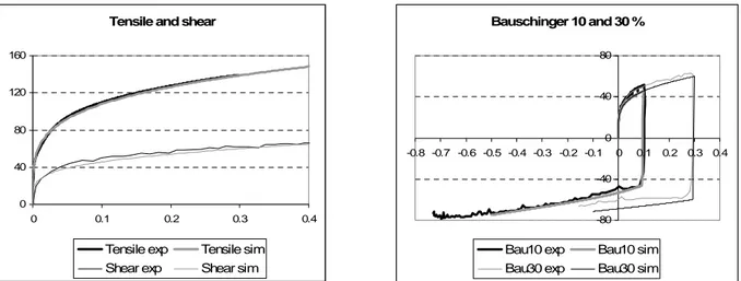
The first identification method consists in performing tensile tests, monotonic shear tests and Bauschinger tests at different amount of pre-strain. The materials parameters are adjusted by inverse method and give a good correlation between experimental and simulation results as shown in Figure 1. Neither kinematic nor mixed hardening is observed for this material, so the isotropic Swift law is fitted:
n p 0 F =K(ε +ε ) σ
with the following material parameters: K= 183 MPa, ε0= 0.00057 and n= 0.229 for the aluminum alloy AA3003-O.
This first set of material data is used to verify the accuracy of the FE prediction compared with the tests performed with the SPIF machine.
Bauschinger 10 and 30 % -80 -40 0 40 80 -0.8 -0.7 -0.6 -0.5 -0.4 -0.3 -0.2 -0.1 0 0.1 0.2 0.3 0.4
Bau10 exp Bau10 sim Bau30 exp Bau30 sim
Tensile and shear
0 40 80 120 160 0 0.1 0.2 0.3 0.4
Tensile exp Tensile sim Shear exp Shear sim
Figure 1. Experimental and simulation tensile, shear and Bauschinger tests
3. INDENT TEST
3.1. Description and results
For the “Indent test” described in Figure 2, the displacements of the four edges of the plate are prevented as the sheet is clamped between a die and a blankholder. The thickness is 1.2 mm. The spherical tool has a radius of 6.35 mm, its initial position is tangent to the top surface of the plate and the indent value is fixed to 10 mm.
230 mm 230 mm X Y tool X Y Z tool Tool side Camera side
Figure 2. Description of the Indent test
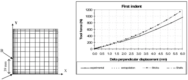
Due to the double symmetry, only a quarter of the plate is considered for the simulations. Two different element types are used: the eight nodes brick elements and the four nodes shell elements. As the goal of the simulation is to identify the law parameters by the inverse method, the meshing is adapted to get a good compromise between accuracy and a short computation time. The same mesh is used in the XY plan (Figure 3) for the two element types: 15 * 15 elements. For the shell elements, only one layer of elements is required while for the bricks, the thickness is divided in three layers. All the nodes along the edges are fixed. The tool force is computed by the implicit static strategy.
The evolution of the tool force is measured with respect to the difference of the displacements in Z direction of two nodes A and B both in the symmetry plane and in the camera side, with A in the center of the plate and B at the distance of 39 mm from A (Figure 3).
Figure 3. Meshing used for the quarter of the plate and simulation results Y X 39 mm A B First indent 0 200 400 600 800 1000 1200 0.0 0.5 1.0 1.5 2.0 2.5 3.0 3.5 4.0 4.5 5.0 5.5 6.0
Delta perpendicular displacement (mm)
T o o l fo rc e (N )
experimental extrapolation Bricks Shells
As observed, the predicted tool force (bricks: 1137.8 N and shells: 1106.5 N) at the end of the indent is higher than the measured force: 920N.
3.2. Effect of numerical and experimental choices on results
The effects of the geometry inaccuracy of the plate (dimension, thickness and flatness) and the tool (initial position and diameter), of the FEM parameters (elements stiffness and number of layers for the bricks), of the sensitivity to the material data (hardening parameters and anisotropy) and of the friction coefficient were examined. All of these parameters had a very small impact on the result observed and couldn’t explain such a gap between FE prediction and experimental results. However, the effect of the boundary conditions described in the next section is a possible explanation.
3.3. New boundary conditions
The impact of a small rotation of the edges is insignificant in sheet simulation while a possible sliding of the edges may explain the gap between the results observed.
Kl
Y
X
Figure 4. New mesh and new boundary conditions
In this new configuration with shell elements, the nodes of the edges are fixed in translation in the Z-direction and in rotation while the displacements in the XY plan are possible and depend on the stiffness of springs (Figure 4). Since the springs should be regularly distributed along the edges to represent the real model, the mesh was modified to get proportional size of elements. At each node of the edges, the number of springs depends on the size of the adjacent elements. This approach allows using the same stiffness for all of the springs.
Using an inverse method, this unique spring stiffness is fitted until reaching the same tool force as the experimental value. The fitted stiffness is 113 N/mm and the spring interval is 0.495 mm. This corresponds to a stiffness of 227.97 N/mm for each mm of edge.
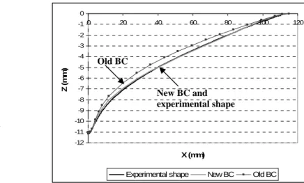
The shape of the plate at the end of the indent is obtained by digital camera pictures. In this case, the shape of a cut in XZ plan was extracted.
This new case (new BC) gives a good prediction of both the force and the shape (Figure 5) while with the old boundary conditions (Old BC) neither the force nor the shape were correct.
X Y A -12 -11 -10 -9 -8 -7 -6 -5 -4 -3 -2 -1 0 0 20 40 60 80 100 120 X (mm) Z ( mm)
Experimental shape New BC Old BC
New BC and experimental shape Old BC
Figure 5. Comparison of the shapes
The maximum sliding with such a model is 0.08 mm for an indent of 10 mm and is located at point A (Figure 5).
To validate the model, this sliding must be compared with the experimental one but it has not yet been measured.
3.4. Inverse method
The indent test does not take into account the Bauschinger effect of the material. It is then not appropriate to fit all the material parameters. Instead, the goal here was to verify the accuracy of the simulations and be prepared for the reverse indent test presented in section 5. 4. LINE TEST
4.1. Description
For the “Line test”, a square plate with a thickness of 1.2 mm is clamped along the edges (Figure 6). The spherical tool radius is 5 mm.
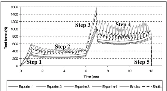
The displacement of the tool is composed of five steps with an initial position tangent to the surface of the plate: a first indent of 5 mm (step 1), a line movement at the same depth along the X axis (step 2), then a second indent until the depth of 10 mm (step 3) followed by a line at the same depth along the X axis (step 4) and the unloading (step5).
Like for the “indent test”, the mesh is adjusted to limit the element number while trying to keep a good accuracy. Two element types are tested: brick with three layers along the thickness and shell elements. The evolution of the tool force is compared with the experimental measurement during the process. The experimental test was performed four times. Figure 7 shows important discrepancy from one test to the others. Up to now, such variability of the experimental tool force has not yet been explained. The simulation results showed in Figure 7 are produced using coarse meshes. The oscillations in the numerical model are due to the contact elements. With a very fine mesh using either bricks or shells, the
force is close to the one related to the shell with a coarse mesh. . 1 3 4 2 1 2 X Y Z tool X Y 182 mm 182 m m tool 100 mm 42 mm 42 mm
Figure 6. Description of the Line test
0 200 400 600 800 1000 1200 1400 1600 0 2 4 6 8 10 12 Time (sec) T o o l fo rc e (N )
Experim 1 Experim 2 Experim 3 Experim 4 Bricks Shells
Step 1
Step 2
Step 3 Step 4
Step 5
Figure 7. Evolution of tool force during the Line test
4.2. Observations
This line test shows that the brick elements are not adapted to such a test because they are not accurate enough when using a coarse mesh. On the other hand, the shell elements predict the same tool force for both the coarse and the very fine mesh. Those elements are also suitable for the inverse method since the computation time is lower than when using the brick elements.
The experimental tests are assumed perfect but the results show that the tests are not reproducible. The discrepancy between simulations and real tests may be explained by a sliding like for the indent test. The measurement of the magnitude of such a movement must still be developed. A new model with new boundary conditions with springs can also be used with an adjusted spring stiffness to reach the experimental tool force.
4.3. Effect of numerical and experimental choice on results
Three element types were tested (two brick and one shell types). For the simulations with bricks, the boundary conditions were also modified by releasing some degrees of freedom along the edges and by taking into account the clamped part of the plate. The results obtained with the classic hardening were compared with the Teodosiu and Ziegler hardenings. None of these parameters could explain the difference between the experimental and the simulation results. The friction effect was also studied. A friction value of 0.15 gives realistic results when comparing the relative intensity of the different components of the tool force with the real one, but the total force is only 1.5 % higher then in the case without friction.
4.4. Inverse method
This line test takes into account the Bauschinger effect, so it should be suitable for the inverse method. The sliding of the edges must be first verified and studied with a new model with springs like for the indent test. It is essential to be able to represent the real process with an accurate tool force and a good shape before using the inverse method.
5. REVERSE INDENT TEST 5.1. Description
The objective of this test is to perform an indent test, as described previously, followed by another indent in the opposite direction to obtain a bending and unbending effect as shown in Figure 8. Experimentally, it is difficult to adjust this test because the positions of the tool must be exactly aligned between the first and the second indent. A small inaccuracy in the position of the tool during the second indent induces warping and a significant deviation of the results. Different tool diameters will be tested to reduce this problem. The indent value will also be adjusted to reach a significant strain level.
The inverse method will be tested to fit the material parameters.
Figure 8. First and second indent tests
6. CONCLUSIONS
The inverse method is a powerful tool for the fitting of complex law parameters like the anisotropic elastic-plastic law based on the HILL48 yield locus used for the simulation of the single point incremental forming. This paper shows that the tests chosen and the numerical parameters of the simulation have a great impact on the material data identification. Therefore, it is essential to verify the reproducibility of the experimental tests and the accuracy of the numerical model used. In the indent and the line tests, the boundary conditions are difficult to adjust, but they may induce a bad prediction of the tool force and a inaccurate data fitting. Therefore, a new configuration with springs along the edges gives a good prediction of both the tool force and the deformed shape. This model must still be validated by measuring the real sliding occurring during the experiments.
In the future, the same boundary conditions will be used for the line test and the reverse indent test. Then, it will be tested if this new model can be used to fit all the material parameters by inverse method.
7. ACKNOWLEDGEMENT
The authors of this article would like to thank the Institute for the Promotion of Innovation by Science and Technology in Flanders (IWT) for their financial support.
As Research Director, A.M. Habraken would like to thank the Fund for Scientific Research (FNRS, Belgium) for its support.
8. REFERENCES
[1] J. Jeswiet, F. Micari, G. Hirt, A. Bramley, J. R. Duflou, J. Allwood, Asymmetric Single
Point Incremental Forming of Sheet Metal, CIRP Annals 2005, Vol. 54/2, Technische
Rundschau, Switzerland, pp. 623-649.
[2] S. He, A. Van Bael, P. Van Houtte, Y. Tunckol, J. Duflou, C. Henrard, C. Bouffioux, A.M. Habraken, Effect of FEM choices in the modelling of incremental forming of
aluminium sheets, Proceedings of the 8th Esaform conference on material forming, Vol.
2, (2005), pp. 711-714
[3] P. Flores, L. Duchene, T. Lelotte, C. Bouffioux, F. El Houdaigui, A. Van Bael, S. He, J. Duflou, A. M. Habraken, Model Identification and FE Simulations: Effect of Different
Yield Loci and Hardening Laws in Sheet Forming, Proceedings of Numisheet 2005, Vol.
A, L. M. Smiths, F. Pourboghrat, J-W. Yoon and T.B. Stoughton (Eds.), pp. 371-381. [4] D. Lecompte, A. Smits, S. Bossuyt, H. Sol, J. Vantomme, D. Van Hemelrijck, A.M.
Habraken, Quality assessment of speckle patterns for digital image correlation, Optics and Lasers in Engineering, Volume 44, Issue 11 (2006), pp. 1132-1145.
[5] S. Cooreman, D. Lecompte, H. Sol, J. Vantomme, D. Debruyne, Elasto-plastic material
parameter identification by inverse methods: Calculation of the sensitivity matrix,
International Journal of Solids and Structures, Available online 18 November 2006, DOI:10.1016/j.ijsolstr.2006.11.024.
[6] R. Hill, The Mathematical Theory of Plasticity, Oxford Engineering Science, Series. Oxford at the Clarendon Press (1950).