• Aucun résultat trouvé

Backtesting Value-at-Risk: A Duration-Based Approach

N/A
N/A
Protected

Academic year: 2021

Partager "Backtesting Value-at-Risk: A Duration-Based Approach"

Copied!
29
0
0

Texte intégral

(1)2003s-05. Backtesting Value-at-Risk: A Duration-Based Approach Peter Christoffersen, Denis Pelletier. Série Scientifique Scientific Series. Montréal Février 2003. © 2003 Peter Christoffersen, Denis Pelletier. Tous droits réservés. All rights reserved. Reproduction partielle permise avec citation du document source, incluant la notice ©. Short sections may be quoted without explicit permission, if full credit, including © notice, is given to the source..

(2) CIRANO Le CIRANO est un organisme sans but lucratif constitué en vertu de la Loi des compagnies du Québec. Le financement de son infrastructure et de ses activités de recherche provient des cotisations de ses organisationsmembres, d’une subvention d’infrastructure du ministère de la Recherche, de la Science et de la Technologie, de même que des subventions et mandats obtenus par ses équipes de recherche. CIRANO is a private non-profit organization incorporated under the Québec Companies Act. Its infrastructure and research activities are funded through fees paid by member organizations, an infrastructure grant from the Ministère de la Recherche, de la Science et de la Technologie, and grants and research mandates obtained by its research teams. Les organisations-partenaires / The Partner Organizations PARTENAIRE MAJEUR . Ministère des Finances, de l’Économie et de la Recherche [MFER] PARTENAIRES . Alcan inc. . Axa Canada . Banque du Canada . Banque Laurentienne du Canada . Banque Nationale du Canada . Banque Royale du Canada . Bell Canada . Bombardier . Bourse de Montréal . Développement des ressources humaines Canada [DRHC] . Fédération des caisses Desjardins du Québec . Gaz Métropolitain . Hydro-Québec . Industrie Canada . Pratt & Whitney Canada Inc. . Raymond Chabot Grant Thornton . Ville de Montréal . École Polytechnique de Montréal . HEC Montréal . Université Concordia . Université de Montréal . Université du Québec à Montréal . Université Laval . Université McGill ASSOCIÉ AU : . Institut de Finance Mathématique de Montréal (IFM2) . Laboratoires universitaires Bell Canada . Réseau de calcul et de modélisation mathématique [RCM2] . Réseau de centres d’excellence MITACS (Les mathématiques des technologies de l’information et des systèmes complexes). Les cahiers de la série scientifique (CS) visent à rendre accessibles des résultats de recherche effectuée au CIRANO afin de susciter échanges et commentaires. Ces cahiers sont écrits dans le style des publications scientifiques. Les idées et les opinions émises sont sous l’unique responsabilité des auteurs et ne représentent pas nécessairement les positions du CIRANO ou de ses partenaires. This paper presents research carried out at CIRANO and aims at encouraging discussion and comment. The observations and viewpoints expressed are the sole responsibility of the authors. They do not necessarily represent positions of CIRANO or its partners.. ISSN 1198-8177.

(3) Backtesting Value-at-Risk: A Duration-Based Approach* Peter Christoffersen†, Denis Pelletier‡. Résumé / Abstract. L'évaluation des modèles de risque financier, ou test inversé, est une partie importante de l'approche avec modèle interne pour la gestion de risque tel qu'établie par le Comité de Basle pour la supervision bancaire (1996). Toutefois, les procédures existantes de tests inversés telles que celles développées dans Christoffersen (1998), ont une puissance relativement faible pour des tailles d'échantillon réalistes. Les méthodes suggérées dans Berkowitz (2001) performe mieux mais sont basées sur de l'information, telle que la forme de la queue gauche de la distribution des rendements du portefeuille, qui n'est pas toujours disponible. La mesure de risque de loin la plus courante est la Valeur-à-Risque (VaR), qui est définie comme un quantile de la distribution conditionnelle du rendement, et elle ne dit rien à-propos de la forme de la distribution à gauche du quantile. Notre contribution est l'exploration d'un nouvel outil pour les tests inversés basé sur la durée en jours entre les violations de la VaR. L'intuition est que si le modèle de VaR est correctement spécifié pour un taux de couverture p, alors la durée espérée conditionnelle entre les violations devrait être une constante 1/p jours. Nous proposons diverses façons de tester cette hypothèse nulle et nous effectuons une analyse Monte Carlo où l'on compare ces nouveaux tests à ceux présentement disponibles. Nos résultats montrent que pour des situations réalistes, les tests basés sur les durées ont de meilleures propriétés en termes de puissance que ceux précédemment proposés. La taille des tests est facilement contrôlée en utilisant la technique Monte Carlo de Dufour (2000). Mots clés : Évaluation de modèle de risque, simulation historique, prévision de densité, test Monte Carlo.. * The first author acknowledges financial support from IFM2, FCAR, and SSHRC, and the second author from FCAR and SSHRC. We are grateful for helpful comments from Frank Diebold, Jean-Marie Dufour, Rob Engle, Eric Ghysels, James MacKinnon, Nour Meddahi, and Matt Pritsker. The usual disclaimer applies. † Corresponding author: Faculty of Management, McGill University, 1001 Sherbrooke Street W., Montreal, Quebec, Canada H3A 1G5. Phone: (514) 398-2869. Fax: (514) 398-3876. Email: Peter.Christoffersen@McGill.ca. ‡ Department de sciences économiques, CP 6128, succursale Centre-Ville, Montreal, Quebec, H3C 3J7, Canada. Email: Denis.Pelletier@UMontreal.ca..

(4) Financial risk model evaluation or backtesting is a key part of the internal model's approach to market risk management as laid out by the Basle Commitee on Banking Supervision (1996). However, existing backtesting methods such as those developed in Christoffersen (1998), have relatively small power in realistic small sample settings. Methods suggested in Berkowitz (2001) fare better, but rely on information such as the shape of the left tail of the portfolio return distribution, which is often not available. By far the most common risk measure is Value-at-Risk (VaR), which is defined as a conditional quantile of the return distribution, and it says nothing about the shape of the tail to the left of the quantile. Our contribution is the exploration of a new tool for backtesting based on the duration of days between the violations of the VaR. The chief insight is that if the VaR model is correctly specified for coverage rate, p, then the conditional expected duration between violations should be a constant 1/p days. We suggest various ways of testing this null hypothesis and we conduct a Monte Carlo analysis which compares the new tests to those currently available. Our results show that in realistic situations, the duration based tests have better power properties than the previously suggested tests. The size of the tests is easily controlled using the Monte Carlo technique of Dufour (2000). Keywords: Risk Model Evaluation, Historical Simulation, Density Forecasting, Monte Carlo Testing..

(5) 1. Motivation. Financial risk model evaluation or backtesting is a key part of the internal model’s approach to market risk management as laid out by the Basle Committee on Banking Supervision (1996). However, existing backtesting methods such as those developed in Christoffersen (1998), has relatively small power in realistic small sample settings. Methods suggested in Berkowitz (2001) fare better, but rely on information such as the shape of the left tail of the portfolio return distribution, which is often not available. By far the most common risk measure is Value-at-Risk (V aR), which is defined as a conditional quantile of the return distribution, and it says nothing about the shape of the tail to the left of the quantile. We will refer to an event where the ex-post portfolio loss exceeds the ex-ante V aR measure as a violation. Of particular importance in backtesting is the clustering of violations. An institution’s internal risk management team as well as external supervisors explicitly want to be able to detect clustering in violations. Large losses which occur in rapid succession are more likely to lead to disastrous events such as bankruptcy. In the previous literature, due to the lack of real portfolio data, the evaluation of V aR techniques were largely based on artificial portfolios. Examples in this tradition include Beder (1995), Christoffersen, Hahn and Inoue (2001), Hendricks (1996), Kupiec (1995), Marshall and Siegel (1997), and Pritsker (1997). But recently, Berkowitz and O’Brien (2002) have reported on the performance of actual V aR forecasts from six large (and anonymous) U.S. commercial banks.1 Figure 1 reproduces a picture from their paper which shows the V aR exceedences from the six banks reported in standard deviations of the portfolio returns. Even though the banks tend to be conservative—they have fewer than expected violations—the exceedences are large and appear to be clustered in time and across banks. From the perspective of a regulator worried about systemic risk, rejecting a particular bank’s risk model due to the clustering of violations is particularly important if the violations also happen to be correlated across banks. The detection of violation clustering is particularly important because of the widespread reliance on V aRs calculated from the so-called Historical Simulation (HS) technique. In the HS methodology, a sample of historical portfolio returns using current portfolio weights is first constructed. The V aR is then simply calculated as the unconditional quantile from the historical sample. The HS method thus largely ignores the last 20 years of academic research on conditional asset return models. Time variability is only captured through the rolling historical sample. In spite of forceful warnings, such as Pritsker (2001), the model-free nature of the HS technique is viewed as a great benefit by many practitioners. The widespread use of HS the technique motivates us to focus attention on backtesting V aRs calculated using this method. 1. Barone-Adesi, Giannopoulos and Vosper (2000) provides another example using real-life portfolio returns.. 1.

(6) While alternative methods for calculating portfolio measures such as the V aR have been investigated in for example Jorion (2000), and Christoffersen (2002), available methods for backtesting are still relatively few. Our contribution is thus the exploration of a new tool for backtesting based on the duration of days between the violations of the risk metric. The chief insight is that if the V aR model is correctly specified for coverage rate, p, then the conditional expected duration between violations should be a constant 1/p days. We suggest various ways of testing this null hypothesis and we conduct a Monte Carlo analysis which compares the new tests to those currently available. Our results show that in many realistic situations, the duration based tests have better power properties than the previously suggested tests. The size of the tests is easily controlled using the Monte Carlo testing approach of Dufour (2000). This procedure is described in detail below. We hasten to add that the sort of omnibus backtesting procedures suggested here are meant as complements to—and not substitutes for—the statistical diagnostic tests carried out on various aspects of the risk model in the model estimation stage. The tests suggested in this paper can be viewed either as a final diagnostic for an internal model builder or alternatively as a feasible diagnostic for an external model evaluator for whom only limited, aggregate portfolio information is available. Our paper is structured as follows: Section 2 outlines the previous first-order Markov tests, Section 3 suggests the new duration-based tests, and Section 4 discusses details related to the implementation of the tests. Section 5 contains Monte Carlo evidence on the performance of the tests. Section 6 suggests various extensions to the analysis, and Section 7 concludes.. 2. Extant Procedures for Backtesting Value-at-Risk. Consider a time series of daily ex-post portfolio returns, Rt , and a corresponding time series of ex-ante Value-at-Risk forecasts, V aRt (p) with promised coverage rate p, such that ideally Prt−1 (Rt < −V aRt (p)) = p. The negative sign arises from the convention of reporting the V aR as a positive number. Define the hit sequence of V aRt violations as ( 1, if Rt < −V aRt (p) It = 0, else Notice that the hit sequence appears to discard a large amount of information regarding the size of violations etc. Recall, however, that the V aR forecast does not promise violations of a certain magnitude, but rather only their conditional frequency, i.e. p. This is a major drawback of the V aR risk measure which we will discuss below. 2.

(7) Christoffersen (1998) tests the null hypothesis that It ∼ i.i.d. Bernoulli(p) against the alternative that It ∼ i.i.d. Bernoulli(π) and refers to this as the test of correct unconditional coverage (uc) H0,uc : π = p which is a test that on average the coverage is correct. The above test implicitly assumes that the hits are independent an assumption which we now test explicitly. In order to test this hypothesis an alternative is defined where the hit sequence follows a first order Markov sequence with switching probability matrix " # 1 − π01 π 01 Π= 1 − π11 π 11 where π ij is the probability of an i on day t − 1 being followed by a j on day t. The test of independence (ind) is then H0,ind : π 01 = π 11 Finally one can combine the two tests in a test of conditional coverage (cc) H0,cc : π 01 = π 11 = p The idea behind the Markov alternative is that clustered violations represent a signal of risk model misspecification. Violation clustering is important as it implies repeated severe capital losses to the institution which together could result in bankruptcy. Notice however, that the Markov first-order alternative may have limited power against general forms of clustering. The first point of this paper is to establish more general tests for clustering which nevertheless only rely on information in the hit sequence.. 3. Duration-Based Tests of Independence. The above tests are reasonably good at catching misspecified risk models when the temporal dependence in the hit-sequence is of a simple first-order Markov structure. However we are interested in developing tests which have power against more general forms of dependence but which still rely only on estimating a few parameters. 3.

(8) The intuition behind the duration-based tests suggested below is that the clustering of no-hit durations will result in an excessive number of relatively short and relatively long durations, corresponding to market turbulence and market calm respectively. Motivated by this intuition we consider the duration of time (in days) between two V aR violations (i.e. the no-hit duration) as Di = ti − ti−1 where ti denotes the day of violation number i.2 Under the null hypothesis that the risk model is correctly specified, the no-hit duration should have no memory and a mean duration of 1/p days. To verify the no memory property note that under the null hypothesis we have the discrete probability distribution Pr (D = 1) = p Pr (D = 2) = (1 − p) p. Pr (D = 2) = (1 − p)2 p .... Pr (D = d) = (1 − p)d−1 p. A duration distribution is often best understood by its hazard function, which has the intuitive definition of the probability of a getting a violation after D days given that we have gone D days without a violation. The above probability distribution implies a flat discrete hazard function as the following derivation shows λ (d) =. Pr (D = d) P 1 − j<d Pr (D = d). (1 − p)d−1 p = P i 1 − d−1 i=1 (1 − p) p. (1 − p)d−1 p = P j 1 − d−2 j=0 (1 − p) p = p. The only memory free (continuous)3 random distribution is the exponential, thus we have that under the null the distribution of the no-hit durations should be fexp (D; p) = p exp (−pD) . 2. For a general introduction to duration modeling, see Kiefer (1988) and Gourieroux (2000). Notice that we use a continuous distribution even though we are counting time in days. This discreteness bias will we acounted for in the Monte Carlo tests. The exponential distribution can also be viewed as the continuous time limit of the above discrete time process. See Poirier (1995). 3. 4.

(9) In order to establish a statistical test for independence we must specify a (parsimonious) alternative which allows for duration dependence. As a very simple case, consider the Weibull distribution where ¡ ¢ fW (D; a, b) = ab bDb−1 exp −(aD)b .. The Weibull distribution has the advantage that the hazard function has a closed form representation, namely fW (D) = ab bDb−1 λW (D) ≡ 1 − FW (D). where the exponential distribution appears as a special case with a flat hazard, when b = 1. The Weibull will have a decreasing hazard function when b < 1, which corresponds to an excessive number of very short durations (very volatile periods) and an excessive number of very long durations (very tranquil periods). This could be evidence of misspecified volatility dynamics in the risk model. Due to the bankruptcy threat from VaR violation clustering the null hypothesis of independence is of particular interest. We therefore want to explicitly test the null hypothesis H0,ind : b = 1. We could also use the Gamma distribution under the alternative hypothesis. The p.d.f. in this case is ab Db−1 exp (−aD) fΓ (D; a, b) = Γ (b). which also nests the exponential when b = 1. In this case we therefore also have the independence test null hypothesis as H0,ind : b = 1. The Gamma distribution does not have a closed-form solution for the hazard function, but the first two moments are ab and ab2 respectively, so the notion of excess dispersion which is defined as the variance over the squared expected value is simply 1b . Note that the average duration in the exponential distribution is 1/p, and the variance of durations is 1/p2 , thus the notion of excess dispersion is 1 in the exponential distribution.. 3.1. A Conditional Duration Test. The above duration tests can potentially capture higher order dependence in the hit sequence by simply testing the unconditional distribution of the durations. Dependence in the hit sequence may show up as an excess of relatively long no-hit durations (quiet periods) and an excess of relatively short no-hit durations, corresponding to violation clustering. However, in the above 5.

(10) tests, any information in the ordering of the durations is completely lost. The information in the temporal ordering of no-hit durations could be captured using the framework of Engle and Russel’s (1998) Exponential Autoregressive Conditional Duration (EACD) model. In the EACD(1,0) model, the conditional expected duration takes the following form Ei−1 [Di ] ≡ ψi = ω + αDi−1 with α ∈ [0, 1) . Assuming an underlying exponential density with mean equal to one, the conditional distribution of the duration is ¶ µ 1 Di exp − fEACD (Di |ψi ) = ψi ψi The null of independent no-hit durations would then correspond to H0,ind : α = 0. Excess dispersion in the EACD(1,0) model is defined as V [Di ]/E[Di ]2 =. 1 1 − 2α2. so that the ratio of the standard deviation to the mean duration is above one if α > 0.. 4. Test Implementation. We will first discuss the specific implementation of the hit sequence tests suggested above. Later, we will simulate observations from a realistic portfolio return process and calculate risk measures from the popular Historical Simulation risk model, which in turn provide us with hit sequences for testing.. 4.1. Implementing the Markov Tests. The log-likelihood function for a sample of T i.i.d. observations from a Bernoulli variable, It , with known probability p is written as ln L (I, p) = pT1 (1 − p)T −T1 where T1 is the number of ones in the sample. The log-likelihood function for an i.i.d. Bernoulli with unknown probability parameter, π 1 , to be estimated is ln L (I, π 1 ) = π T1 1 (1 − π 1 )T −T1 . 6.

(11) The ML estimate of π 1 is π ˆ 1 = T1 /T and we can thus write a likelihood ratio test of unconditional coverage as ˆ 1 ) − ln L (I, p)) . LRuc = −2 (ln L (I, π For the independence test, the likelihood under the alternative hypothesis is ln L (I, π 01 , π 11 ) = (1 − π01 )T0 −T01 πT0101 (1 − π 11 )T1 −T11 π T1111 where Tij denotes the number of observations with a j following an i. The ML estimates are π ˆ 01 = T01 /T0 π ˆ 11 = T11 /T1 and the independence test statistic is ˆ 01 , π ˆ 11 ) − ln L (I, π ˆ 1 )) . LRind = −2 (ln L (I, π Finally the test of conditional coverage is written as ˆ 01 , π ˆ 11 ) − ln L (I, p)) . LRcc = −2 (ln L (I, π We note that all the tests are carried out conditioning on the first observation. The tests are asymptotically distributed as χ2 with degree of freedom one for the uc and ind tests and two for the cc test. But we will instead rely on finite sample p-values below. Finally, as a practical matter, if the sample at hand has T11 = 0, which can easily happen in small samples and with small coverage rates, then we calculate the first-order Markov likelihood as ln L (I, π01 , π 11 ) = (1 − π 01 )T0 −T01 π T0101 and carry out the tests as above.. 4.2. Implementing the Weibull and EACD Tests. In order to implement our tests based on the duration between violations we first need to transform the hit sequence into a duration series Di . While doing this transformation we also create the series Ci to indicate if a duration is censored (Ci = 1) or not (Ci = 0). Except for the first and last duration the procedure is straightforward, we just count the number of days between each violation and set Ci = 0. For the first observation if the hit sequence starts with 0 then 7.

(12) D1 is the number of days until we get the first hit. Accordingly C1 = 1 because the observed duration is left-censored. If instead the hit sequence starts with a 1 then D1 is simply the number of days until the second hit and C1 = 0. The procedure is similar for the last duration. If the last observation of the hit sequence is 0 then the last duration, DN(T ) , is the number of days after the last 1 in the hit sequence and CN(T ) = 1 because the spell is right-censored. In the same manner if the last observation of the hit sequence is a 1 then DN(T ) = tN(T ) − tN(T )−1 and CN (T ) = 0. The contribution to the likelihood of an uncensored observation is its corresponding p.d.f. For a censored observation, we merely know that the process lasted at least D1 or DN (T ) so the contribution to the likelihood is not the p.d.f. but its survival function S(Di ) = 1 − F (Di ). Combining the censored and uncensored observations, the log-likelihood is N(T )−1. L(D; Θ) = C1 ln S(D1 ) + (1 − C1 ) ln f (D1 ) +. X. ln(f (Di )). i=2. +CN(T ) ln S(DN (T ) ) + (1 − CN(T ) ) ln f (DN(T ) ). Once the durations are computed and the truncations taken care of, then the likelihood ratio tests can be calculated in a straightforward fashion. The only added complication is that the ML estimates are no longer available in closed form, they must be found using numerical optimization.. 4.3. Finite Sample Inference. While the large-sample distributions of the likelihood ratio tests we have suggested above are well-known,4 they may not lead to reliable inference in realistic risk management settings. The nominal sample sizes can be reasonably large, say two to four years of daily data, but the scarcity of violations of for example the 1% V aR renders the effective sample size small. In this section, we therefore present the technique of Monte Carlo tests [see Dufour (2000)]. For the case of a continuous test statistic, the procedure is the following. We first generate N independent realizations of the test statistic, LRi , i = 1, . . . , N . We denote by LR0 the test computed with the original sample. Under the hypothesis that the risk model is correct we know that the hit sequence is i.i.d. Bernoulli with the mean equal to the coverage rate in our application. We thus benefit from the advantage of not having nuisance parameters under the null hypothesis. 4. Testing α = 0 in the EACD(1,0) model presents a potential difficulty asymptotically in that it is on the boundary of the parameter space.. 8.

(13) We next rank LRi , i = 0, . . . , N in non-decreasing order and obtain the Monte Carlo p-value pˆN (LR0 ) where ˆ N (LR0 ) + 1 NG pˆN (LR0 ) = N +1 with N 1 X ˆ GN (LR0 ) = 1 (LRi > LR0 ) N i=1. where 1 (∗) takes on the value 1 if ∗ is true and the value 0 otherwise. When working with binary sequences the test values can only take a countable number of distinct values. Therefore, we need a rule to break ties between the test value obtained from the sample and those obtained from Monte Carlo simulation under the null hypothesis. The tie-breaking procedure is as follows: For each test statistic, LRi , i = 0, . . . , N , we draw an independent realization of a Uniform distribution on the [0; 1] interval. Denote these draws by Ui , i = 0, . . . , N . The Monte-Carlo p-value is now given by p˜N (LR0 ) = with. 5. ˜ N (LR0 ) + 1 NG N +1. N N X 1 X ˜ N (LR0 ) = 1 − 1 1 (LRi < LR0 ) + 1 (LRi = LR0 ) 1 (Ui ≥ U0 ) . G N i=1 N i=1. Backtesting V aRs from Historical Simulation. We now assess the power of the proposed duration tests in the context of a Monte Carlo study. Consider a portfolio where the returns are drawn from a GARCH(1,1)-t(d) model with leverage, that is p ((ν − 2) /ν)zt+1 , with ´2 ³p = ω + ασ 2t ((ν − 2) /ν)zt − θ + βσ 2t. Rt+1 = σ t+1 σ 2t+1. where the innovation zt+1 ’s are drawn independently from a Student’s t (ν) distribution. Notice that the innovations have been rescaled to ensure that the conditional variance of return will be σ 2t+1 .. 9.

(14) In the simulations below we choose the following parameterization α = 0.1 θ = 0.5 β = 0.85 ω = 3.9683e − 6 ν = 8 where ω is set to target an annual standard deviation of 0.20. The parameters imply a daily volatility persistence of 0.975, a mean of zero, a conditional skewness of zero, and a conditional (excess) kurtosis of 1.5. This particular DGP is constructed to form a realistic representation of an equity portfolio return distribution. The risk measurement method under study is the popular Historical Simulation (HS) technique. It takes the Value at Risk on a certain day to be simply the unconditional quantile of the past Te daily observations. Specifically p V aRt+1 = −P ercentile({Rτ }tτ =t−Te +1 , 100p).. From the return sample and the above V aR, we are implicitly assuming that $1 is invested each day. Equivalently, the V aR can be interpreted as being calculated in percent of the portfolio value. In practice, the sample size is often determined by practical considerations such as the amount of effort involved in valuing the current portfolio holdings using past prices on the underlying securities. For the purposes of this Monte Carlo experiment, we set Te = 250 or Te = 500 corresponding to roughly one or two years of trading days. The V aR coverage rate, p, is typically chosen in practice to be either 1% or 5%, and below we assess the power to reject the HS model using either of those rates. Figure 2 shows a return sample path from the above GARCH-t(d) process along with the 1% and 5% V aRs from the HS model (with Te = 500). Notice the peculiar step-shaped V aRs resulting from the HS method. Notice also the infrequent changes in the 1% V aR. The V aR exceedences from the return sample path and the 1% V aR are shown in Figure 3 reported in daily standard deviations of returns. The simulated data in Figure 3 can thus be compared with the real-life data in Figure 1, which was taken from Berkowitz and O’Brien (2002). The clustering and the magnitude of the exceedences are quite similar across the two plots. Note that we have simulated 1,000 observations in Figure 3, while Figure 1 contains between 550 and 750 observations per bank. Figure 3 contains more violations than Figure 1 because of these differences in the sample size and because the banks in Figure 1 tend to report V aRs which on average lead to fewer than p violations. 10.

(15) Before assessing the finite sample power results we simulate one very long realization (5 million observations) of the GARCH return process and calculate 1% and 5% V aRs from Historical Simulation with a rolling set of 500 in-sample returns. The zero-one hit sequence is then calculated from the ex-post daily returns and the ex-ante V aRs. Figure 4 plots the hazard functions of the duration between violations in the long simulation of GARCH data and Historical Simulation V aRs. The hazard from the 1% V aR is shown in the top panel, and the 5% V aR in the bottom panel. The hazard functions are estimated nonparametrically via the Kaplan-Meier product-limit estimator of the survival function, which is described in Kiefer (1988). These hazards are estimated over intervals of 15 days so if there is a probability p of getting a hit at each day then the probability that a given duration will last less than 15 days is 15 X. Pr(D = i) =. i=1. 15 X (1 − p)i−1 p i=1. = 1 − (1 − p)15 .. For p equal to 1% and 5% we get a constant hazard of 0.14 and 0.54 respectively over a 15-day interval. We see in Figure 4 that the estimated hazard is at first bigger and then lower than what we would get with a constant probability of getting a hit. Notice the distinctly downward sloping hazard functions, which correspond to positive duration dependence. Finally, Figure 5 shows the simple histograms of durations between the violations. The top panel again shows the 1% V aR and the bottom panel shows the 5% V aR. Data and other resource constraints often force risk managers to backtest their models on a relatively limited backtesting samples. We therefore conduct our power experiment with samples sizes from 500 to 1500 days in increments of 250 days. Thus our backtesting samples correspond to approximately two through six years. Below we simulate GARCH returns, calculate HS V aRs and the various test statistics over 1,000 Monte Carlo replications. The power of the tests are then simply calculated as the number of simulations, divided by 1000, in which the Monte Carlo p-value is smaller than the chosen level. The rejection frequencies are calculated at the 1%, 5% and 10% significance levels. In order to compute p-values we simulate N = 9999 hit sequence samples under the null hypothesis that the sequences are distributed i.i.d. Bernoulli(p). In order to make sure that we can calculate the test statistics, we do not use Monte Carlo samples with zero or one V aR violations.5 This of course constitutes a nontrivial sample selection rule for the smallest sample sizes and the 1% V aR coverage rate. As it is done for all the tests 5. The likelihood of the Weibull distribution can be unbounded when we have only one uncensored observation. When it happens we discard the sample. We get an unbounded likelihood for less than 3% of the draws when the. 11.

(16) considered, the results are still comparable across tests. It also appears to be realistic that a risk management team would not start backtesting unless at least a couple of violations had occurred. The rejection frequencies below reflect this sample selection which is particularly important for the low (e.g. 1%) V aR coverage rates and in the smallest samples (500 observations).. 5.1. Results. The results of the Monte Carlo simulations are presented in Tables 1 and 2. We report the empirical rejection frequencies (power) for the Markov, Weibull and EACD independence tests for various significance test levels, V aR coverage rates, and backtesting sample sizes. Table 1 reports power for a Historical Simulation Risk model with Te = 500 rolling estimation sample observations and Table 2 for Te = 250 rolling estimation sample observations.6 The results are quite striking. The main result is that the Weibull test is virtually almost more powerful than the Markov and EACD tests in rejecting the HS risk models. This result holds across inference sample sizes, VaR coverage rates and significance levels chosen. The only two exceptions occur in Table 1 for a significance level of 1%, a coverage rate of 5% and a sample of 500 where the EACD is better and in Table 1 for a significance level of 1%, a coverage rate of 1% and a sample of 500 where the Markov test is slightly better. The differences in power are sometimes very large. For example in Table 1 using a 1% significance level, the 5% VaR in a sample of 1,250 observations has a Weibull rejection frequency of 65.2% and a Markov rejection frequency of only 29.8%. The Weibull test clearly appears to pick up dependence in the hit violations which is ignored by the Markov test. The performance of the EACD test on the other hand is quite sporadic. It appears to do quite well at smaller sample sizes but relatively poorly at larger sample sizes. We suspect that the nonlinear estimate of the α parameter is poorly behaved. Note that the rejection frequencies for a given test are not always increasing in inference sample size. This is due to the sample selection procedure in which we discard samples with less than two violations. This sample selection is going to increase power ceteris paribus, and it is going to have the biggest effect in cells corresponding to the fewest average number of violations. These are of course the smallest sample sizes and the smallest coverage rate. Comparing rejection frequencies across coverage rates in Table 1 we also note that in small samples the power is sometimes higher for the 1% VaR coverage rate than for the corresponding coverage rate is 1% and the sample size is 500, and the probability is smaller than 0.5% for higher coverage rates and sample sizes. 6 We focus solely on the independence tests here because the historical simulation risk models under study are correctly specified unconditionally.. 12.

(17) 5% VaR. This may appear to be surprising as the hit sequences from the 5% VaRs contain many more violations which is the source of power. But the sample selection procedure will again have the largest effect for the 1% coverage rate and for the smallest samples. The selected samples for 1% coverage will thus tend to display more dependence on average than those selected for 5% coverage rate. Comparing numbers across Tables 1 and 2, we note that for a coverage rate of 1% the HS VaR with Te = 500 rolling sample observations always has a higher rejection frequency than the HS VaR with Te = 250 rolling sample observations. This result is interesting because practitioners often work very hard to expand their data bases enabling them to increase their rolling estimation sample period. Our results indicate that such efforts may be futile. When the return volatility process is very persistent, it is better to use a relatively short rolling estimation sample period.. 6. Possible Extensions. 6.1. The Monte Carlo Study. Encouraged by the results in Tables 1-2, we now briefly outline some possible extensions to the Monte Carlo study: • We only investigated one particular parameterization of the GARCH process above. It may be interesting to calculate the power of the test for processes with different volatility persistence, different degrees of conditional kurtosis and different leverage effects. • One could also consider more elaborate data generating processes. Engle and Lee (1999) consider a component GARCH model which delivers long-memory like patterns in volatility. Hansen (1994) considers GARCH-t(vt ) models where the degrees of freedom, ν t , varies over time in an autoregressive fashion. • Structural breaks in the underlying return models, such as those investigated by Andreou and Ghysels (2002), may be of interest as well. • Hamilton and Jorda (2002) have recently introduced a class of dynamic hazard models. Exploring these for the purpose of backtesting could be interesting. Finally, before even venturing into the backtesting of actual risk models it may be useful to conduct a more basic Monte Carlo analysis drawing violation sequences and duration data directly. Specifically, if the violation sequence is generated by a first-order Markov process, what is then the power of the different tests? Conversely, if the violation sequence is constructed from simulated duration data with dependence, then what would the power of the different tests be? 13.

(18) 6.2. Backtesting Tail Density Forecasts. The choice of Value-at-Risk as a portfolio risk measure can be criticized on several fronts. Most importantly, the quantile nature of the V aR implies that the shape of the return distribution to the left of the left is ignored. Particularly in portfolio’s with highly nonlinear distributions, such as those including options, this shortcoming can be crucial. Theoreticians have criticized the V aR measure both from a utility-theoretic perspective (Artzner et al, 1999) and from a dynamic trading perspective (Basak and Shapiro, 2000). Although some of these criticisms have recently been challenged (Cuoco, He, and Issaenko, 2001), it is safe to say that risk managers ought to be interested in knowing the entire distribution of returns, and in particular the left tail. Backtesting distributions rather than V aRs then becomes important. Consider the standard density forecast evaluation approach7 of calculating the uniform transform variable Ut = Ft (Rt ) where Ft (∗) is the a priori density forecast for time t. The null hypothesis that the density forecast is optimal corresponds to Ut ∼ i.i.d. Unif orm(0, 1) Berkowitz (2001) argues that the bounded support of the uniform variable renders standard inference difficult. One is forced to rely on nonparametric tests which have notoriously poor small sample properties. He suggests a simple transformation using the inverse normal c.d.f. Zt = Φ−1 (Ut ) after which the hypothesis Zt ∼ i.i.d. Normal(0, 1) can easily be tested. Berkowitz further argues that confining attention to the left tail of the distribution has particular merit in the backtesting of risk models where the left tail contains the largest losses, which are most likely to impose bankruptcy risk. He defines the censored variable ( Zt , if Rt < V aRt ∗ Zt = Φ−1 (V aRt ) , else and tests the null that Zt∗ ∼ Censored Normal(0, 1, V aRt ) 7. See for example Diebold, Gunther and Tay (1998).. 14.

(19) We note first that Berkowitz (2001) only tests the unconditional distribution of Zt∗ . The information in the potential clustering of the V aR exceedences is ignored. Second, note that the censored variable complication is not needed. If we want to test that the transforms of the p100 largest losses are themselves uniform, then we can simply multiply the subset of the uniform by 1/p, apply the transformation and test for standard normality again.8 That is ( Ut /p, if Rt < V aRt ∗∗ Ui = Else not defined We then have that Zi∗∗ = Φ−1 (Ui∗∗ ) ∼ i.i.d. Normal(0, 1) Note that due to the censoring there is no notion of time in the sequence Zi∗∗ . We might want to make a joint analysis of both Zi∗∗ and the duration between violations Di . To do this we would like to write a joint density for these two processes under the alternative. We know that under the null hypothesis that the risk model is correctly specified the Zi∗∗ should be i.i.d. N(0, 1), Di should be i.i.d. exponential with mean 1/p, and the processes should be independent. The question is how to write a joint density for these two processes as the alternative hypothesis knowing that, for example, the marginal p.d.f. of Di is a Weibull and some other p.d.f. for Zi∗∗ ? Copulas provide a useful tool for doing so. A (bivariate) copula is a function C from [0; 1] × [0; 1] to [0; 1] with the following properties: 1. For every u, v in [0; 1], C(u, 0) = 0 = C(0, v) and C(u, 1) = u and C(1, v) = v; 2. For every u1 , u2 , v1 , v2 in [0; 1] such that u1 ≤ u2 and v1 ≤ v2 , C(u2 , v2 ) − C(u2 , v1 ) − C(u1 , v2 ) + C(u1 , v1 ) ≥ 0 In order to explain how copulas can be used we apply Sklar’s theorem (Nelsen, 1998), which states: Let H be a joint distribution function with margins F and G. Then there exists a copula C such that for all x, y in R, H(x, y) = C(F (x), G(y)). If F and G are continuous then C is unique. Conversely, if C is a copula and F and G are distribution functions then H is a joint distribution function with marginal densities F and G. 8. We are grateful to Nour Meddahi for pointing this out.. 15.

(20) So if we have two densities under the alternative (e.g. f (Di ) and g(Zi∗∗ )) then we can easily construct a joint density by applying a copula. Suppose the considered bivariate copula C(u, v; θ) is a function of a unique parameter θ and that we have C(u, v; θ0 ) = uv and C(u, v; θ) 6= uv for θ 6= θ0 . This gives us a basis for a test because C(F (x), G(y); θ0 ) = F (x)G(y) means that x and y are independent. An example of such a copula is the Ali-Mikhail-Haq family of copulas where C(u, v; θ) =. uv ; 1 − θ(1 − u)(1 − v). θ ∈ [−1, 1]. and we have C(u, v; θ) = uv if θ = 0. A possible alternative hypothesis could be that Di is i.i.d. Weibull(a, b), Zi∗∗ is i.i.d. N(µ, σ 2 ) and C(u, v; θ) is from the Ali-Mikhail-Haq family of copulas. We could then test H0. :. a = p, b = 1, µ = 0, σ = 1, θ = 0. H1. :. at least one of these equalities does not hold. in a likelihood ratio framework similar to the one considered for the V aR tests above. We plan to the pursue the implementation of such tests in future work.. 7. Summary. We have presented a new set of procedures for backtesting risk models. The chief insight is that if the V aR model is correctly specified for coverage rate, p, then the conditional expected duration between violations should be a constant 1/p days. We suggest various ways of testing this null hypothesis and we conduct a Monte Carlo analysis which compares the new tests to those currently available. Our results show that in many of the situations we consider, the duration based tests have much better power properties than the previously suggested tests. The size of the tests is easily controlled through finite sample p-values, which we calculate using Monte Carlo simulation. The immediate potential extensions to our Monte Carlo results are many. We could consider alternative data generating processes for returns and alternative risk models. Allowing for realistic nonstationarities such as structural breaks in the return process could be interesting as well. The majority of financial institutions use V aR as a risk measure, and many calculate VaR using the so-called Historical Simulation approach. While the main focus of our paper has thus been backtesting V aRs from Historical Simulation, we also suggest extensions to density and density tail backtesting. 16.

(21) References [1] Andreou and Ghysels (2002), Quality Control for Value at Risk: Monitoring Disruptions in the Distribution of Risk Exposure, Manuscript, University of North Carolina. [2] Artzner, P., F. Delbaen, J.-M. Eber and D. Heath (1999), Coherent Measures of Risk, Mathematical Finance, 9, 203-228. [3] Barone-Adesi, G., K. Giannopoulos and L. Vosper (2000), Backtesting Derivative Portfolios with FHS, Manuscript, USI and City Business School. [4] Basak, S. and A. Shapiro (2000), Value at Risk Based Risk Management: Optimal Policies and Asset Prices, Review of Financial Studies, 14, 371-405. [5] Basle Committee on Banking Supervision (1996), Amendment to the Capital Accord to Incorporate Market Risks. Basle. [6] Beder, T. (1995), VaR: Seductive but Dangerous, Financial Analysts Journal, SeptemberOctober, 12-24. [7] Berkowitz, J. (2001), Testing Density Forecasts, Applications to Risk Management Journal of Business and Economic Statistics, 19, 465-474. [8] Berkowitz, J. and J. O’Brien (2002), How Accurate are the Value-at-Risk Models at Commercial Banks? Journal of Finance, 57, 1093-1112. [9] Christoffersen, P. (1998), Evaluating Interval Forecasts, International Economic Review, 39, 841-862. [10] Christoffersen, P. (2002), Elements of Financial Risk Management, Academic Press, Forthcoming. [11] Christoffersen, P., J. Hahn and A. Inoue (2001), Testing and Comparing Value-at-Risk Measures Journal of Empirical Finance, 8, 325-342. [12] Cuoco, D., H. He, and S. Issaenko (2001), Optimal Dynamic Trading Strategies with Risk Limits, Manuscript, Yale University. [13] Diebold, F.X., T. Gunther, and A. Tay (1998), Evaluating Density Forecasts, with Applications to Financial Risk Management, International Economic Review, 39, 863-883 .. 17.

(22) [14] Dufour, J.-M. (2000), Monte Carlo Tests with Nuisance Parameters : A General Approach to Finite-Sample Inference and Nonstandard Asymptotics in Econometrics, Manuscript, Université de Montréal. [15] Engle, R. and G.J. Lee (1999), A Permanent and Transitory Component Model of Stock Return Volatility, in ed. R. Engle and H. White Cointegration, Causality, and Forecasting: A Festschrift in Honor of Clive W.J. Granger, Oxford University Press, 475-497. [16] Engle, R. and J. Russel (1998), Autoregressive Conditional Duration: A New Model for Irregularly Spaced Transaction Data, Econometrica, 66, 1127-1162. [17] Gourieroux, C. (2000) Econometrics of Qualitative Dependent Variables. Translated by Paul B. Klassen. Cambridge University Press. [18] Hamilton, J. and O. Jorda (2002), A Model for the Federal Funds Rate Target, Journal of Political Economy. Forthcoming. [19] Hansen, B. (1994), Autoregressive Conditional Density Estimation, International Economic Review, 35, 705-730. [20] Hendricks, D. (1996), Evaluation of Value-at-Risk Models Using Historical Data, Economic Policy Review, Federal Reserve Bank of New York, April, 39-69. [21] Kiefer, N. (1988), Economic Duration Data and Hazard Functions, Journal of Economic Literature, 26, 646-679. [22] Kupiec, P. (1995), Techniques for Verifying the Accuracy of Risk Measurement Models, Journal of Derivatives, 3, 73-84. [23] Jorion, P. (2000), Value-at-Risk: The New Benchmark for Controlling Financial Risk. Chicago: McGraw-Hlill. [24] Nelsen, R.(1998), An Introduction to Copulas, Lectures Notes in Statistics, 139, Springer Verlag. [25] Poirier, D. (1995), Intermediate Statistics and Econometrics: A Comparative Approach. Cambridge, MA: MIT Press. [26] Pritsker, M. (1997), Evaluating Value at Risk Methodologies: Accuracy versus Computational Time, Journal of Financial Services Research, 201-241. [27] Pritsker, M. (2001), The Hidden Dangers of Historical Simulation, Manuscript, Federal Reserve Board. 18.

(23) Figure 1 Value-at-Risk Exceedences From Six Major Commercial Banks Berkowitz and O’Brien (2002). 19.

(24) Figure 2 GARCH-t(d) Simulated Portfolio Returns with 1% and 5% Value-at-Risk from Historical Simulation with Te = 500. 0.08. 0.06. 0.04. 0.02. 0. -0.02. -0.04. -0.06. -0.08. -0.1. 0. 100. 200. 300. 400. 500. 20. 600. 700. 800. 900. 1000.

(25) Figure 3 GARCH-t(d) Simulated Portfolio Returns with Exeedences of 1% V aRs from Historical Simulation with Te = 500 Reported in Standard Deviations of Returns. 0. -0.5. -1. -1.5. -2. -2.5. -3. -3.5. 0. 100. 200. 300. 400. 500. 21. 600. 700. 800. 900. 1000.

(26) Figure 4 Hazard Functions of Duration between V aR Violations GARCH-t(d) Portfolio Returns Historical Simulation Risk Model with Te = 500. 1% Value-at-Risk 1 0.8 0.6 0.4 0.2 0. 50. 100. 150. 200. 250. 200. 250. 5% Value-at-Risk 1 0.8 0.6 0.4 0.2 0. 50. 100. 150. 22.

(27) Figure 5 Histograms of Duration between V aR Violations GARCH-t(d) Portfolio Returns Historical Simulation Risk Model with Te = 500. 1% Value-at-Risk 1 0.8 0.6 0.4 0.2 0. 25. 75. 125. 175. 225. 275. 325. 375. 425. 475. 525. 575. 625. 675. 725. 475. 525. 575. 625. 675. 725. 5% Value-at-Risk 1 0.8 0.6 0.4 0.2 0. 25. 75. 125. 175. 225. 275. 325. 375. 23. 425.

(28) Table 1: Empirical Power in Independence Tests: Historical Simulation with Te = 500 Significance Level: 1% Coverage Rate: 1%. Significance Level: 5% Coverage Rate: 1%. Significance Level: 10% Coverage Rate: 1%. Test: Markov Weibull EACD Test: Markov Weibull EACD Test: Markov Weibull EACD Sample size Sample size Sample size 500 750. 0.1190 0.1450. 0.1790 0.2510. 0.1530 0.1840. 500 750. 0.3320 0.2940. 0.3520 0.4850. 0.2510 0.2560. 500 750. 0.4210 0.4620. 0.4690 0.5840. 0.3100 0.3270. 1000 1250. 0.1950 0.2480. 0.3800 0.4840. 0.1240 0.1600. 1000 1250. 0.3320 0.3750. 0.5900 0.6750. 0.2300 0.2590. 1000 1250. 0.4960 0.5090. 0.6730 0.7550. 0.2770 0.3220. 1500. 0.2930. 0.6030. 0.1300. 1500. 0.4020. 0.7550. 0.2150. 1500. 0.5310. 0.8200. 0.2600. Coverage Rate: 5% Test: Markov Weibull EACD Sample size 500. 0.2120. 0.2770. 750 1000. 0.2720 0.3090. 1250 1500. 0.3970 0.4190. Coverage Rate: 5% Test: Markov Weibull EACD. 0.3290. Sample size 500. 0.3010. 0.4560. 0.4610 0.6070. 0.4030 0.4120. 750 1000. 0.3690 0.4090. 0.6760 0.7650. 0.5220 0.4840. 1250 1500. 0.5530 0.6360. Coverage Rate: 5% Test: Markov Weibull EACD. 0.4320. Sample size 500. 0.3600. 0.5390. 0.4880. 0.6410 0.7670. 0.5170 0.5630. 750 1000. 0.4420 0.4920. 0.7390 0.8280. 0.5940 0.6280. 0.8370 0.8970. 0.6380 0.6180. 1250 1500. 0.6720 0.7220. 0.8920 0.9330. 0.6970 0.6800.

(29) Table 2: Empirical Power in Independence Tests: Historical Simulation with Te = 250 Significance Level: 1% Coverage Rate: 1%. Significance Level: 5% Coverage Rate: 1%. Significance Level: 10% Coverage Rate: 1%. Test: Markov Weibull EACD Test: Markov Weibull EACD Test: Markov Weibull EACD Sample size Sample size Sample size 500 750. 0.0990 0.0940. 0.1040 0.0890. 0.0720 0.0560. 500 750. 0.2460 0.2340. 0.2560 0.2880. 0.1540 0.1100. 500 750. 0.2830 0.3050. 0.3530 0.4100. 0.2030 0.1650. 1000 1250. 0.1110 0.1390. 0.1690 0.2240. 0.0420 0.0240. 1000 1250. 0.2720 0.2990. 0.3480 0.4620. 0.1100 0.0700. 1000 1250. 0.3750 0.4080. 0.4800 0.5630. 0.1430 0.1120. 1500. 0.1880. 0.3350. 0.0180. 1500. 0.3200. 0.5360. 0.0590. 1500. 0.4610. 0.6370. 0.0960. Coverage Rate: 5% Test: Markov Weibull EACD Sample size 500. 0.1970. 0.3030. 750 1000. 0.2540 0.3060. 1250 1500. 0.2980 0.3700. Coverage Rate: 5% Test: Markov Weibull EACD. 0.2990. Sample size 500. 0.2830. 0.4660. 0.4230 0.5670. 0.3510 0.3470. 750 1000. 0.3720 0.4150. 0.6520 0.7300. 0.3570 0.3830. 1250 1500. 0.4890 0.6020. Coverage Rate: 5% Test: Markov Weibull EACD. 0.4310. Sample size 500. 0.3480. 0.5520. 0.4780. 0.6360 0.7420. 0.4790 0.4750. 750 1000. 0.4100 0.5070. 0.7300 0.8170. 0.5380 0.5340. 0.8110 0.8770. 0.4880 0.5280. 1250 1500. 0.6070 0.7120. 0.8680 0.9150. 0.5380 0.6130.

(30)

Figure

Table 1: Empirical Power in Independence Tests: Historical Simulation with T e = 500
Table 2: Empirical Power in Independence Tests: Historical Simulation with T e = 250

Références

Documents relatifs

In addition, the existing tests can be used to identify relevant pieces of model executions that make it possible to reach a given state in the property automaton, helping

a backtesting sample size of 250, the LR independence tests have an e¤ec- tive power that ranges from 4.6% (continuous Weibull test) to 7.3% (discrete Weibull test) for a

‘ Density Forecast Evaluation’ approach to the assessment of the tail of return distribution only, we suggest adapting a test of the ‘ Event Probability Forecast

13 conditional coverage tests are used, namely 7 dynamic binary specifications DB, 6 DQ tests (Engle and Manganelli, 2004) including several lags of the violations variable and VaR,

In fact, a model that does not satisfy the independence property can lead to clusterings of margin exceedances even if it has the correct average number of violations.. (7) This

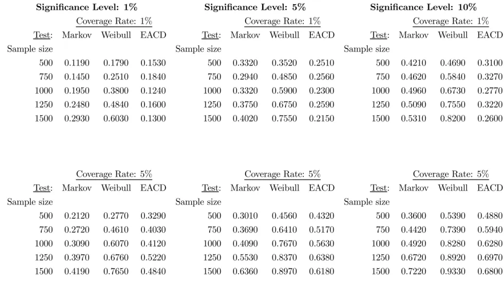
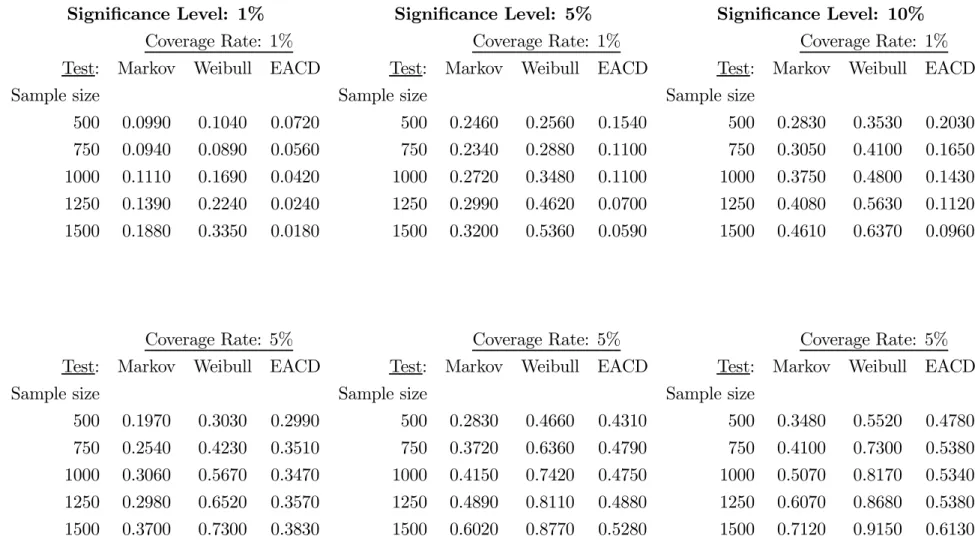
On the contrary, the backtests based on bootstrap critical values display empirical sizes that are close to the nominal size of 5% for all reported sample sizes and risk levels..

Gwenaël PIGANEAU, Directeur de recherche, CNRS Adam EYRE-WALKER, Professor, University of Sussex Carole SMADJA, Chargée de recherche, CNRS Laurent DURET, Directeur de recherche,

This dissimilarity measure is used in conjunction with the McDiarmid Theorem within the a contrario approach in order to design a robust Variable Size Block Matching (VSBM)