Cerebral functional connectivity periodically (de)synchronizes with anatomical
constraints
Rapha¨el Li´egeoisa,1, Erik Zieglerb, Pierre Geurtsa, Francisco Gomezb,c, Mohamed Ali Bahrib, Christophe Phillipsa,b, Andrea Soddud, Audrey Vanhaudenhuysee, Steven Laureysb, Rodolphe Sepulchrea,f
aDepartment of Electrical Engineering and Computer Science, University of Li`ege, Li`ege, Belgium bCyclotron Research Centre, University of Li`ege, Li`ege, Belgium
cComputer Science Department, Universidad Central de Colombia, Bogot´a, Colombia
dMind & Brain Institute, Department of Physics and Astronomy, Western University, London, ON, Canada eDepartment of Algology and Palliative Care, University Hospital of Li`ege, Li`ege, Belgium
fDepartment of Engineering, Trumpington Street, University of Cambridge, Cambridge CB2 1PZ, United Kingdom
Abstract
This paper studies the link between resting-state functional connectivity (FC), measured by the correlations of the fMRI BOLD time courses, and structural connectivity (SC), estimated through fiber tractography. Instead of a static analysis based on the correlation between SC and the FC averaged over the entire fMRI time series, we propose a dynamic analysis, based on the time evolution of the correlation between SC and a suitably windowed FC. Assessing the statistical significance of the time series against random phase permutations, our data show a pronounced peak of significance for time window widths around 20-30 TR (40-60 sec). Using the appropriate window width, we show that FC patterns oscillate between phases of high modularity, primarily shaped by anatomy, and phases of low modularity, primarily shaped by inter-network connectivity. Building upon recent results in dynamic FC, this emphasizes the potential role of SC as a transitory architecture between different highly connected resting state FC patterns. Finally, we show that networks implied in consciousness-related processes, such as the default mode network (DMN), contribute more to these brain-level fluctuations compared to other networks, such as the motor or somatosensory networks. This suggests that the fluctuations between FC and SC are capturing mind-wandering effects.
Keywords: functional connectivity, structural connectivity, dynamics, spontaneous activity, fMRI, DWI, windowing, multimodal imaging, mind wandering.
Introduction
The human brain shows organized spatio-temporal activity even in task-free or “resting-state” conditions which is characterized by very slow (< 0.1Hz) fluctuations of the fMRI Blood Oxygen Level Dependent (BOLD) signal (Gusnard et al., 2001; Greicius et al., 2003). Separate and spatially distinct cerebral regions have also been shown to exhibit coherent activity patterns as measured by the correlation between regional fMRI BOLD time series. This measure of so-called functional connectivity (FC) (see Friston (2011) for a review) is organized in robust resting-state networks (Beckmann et al., 2005; Damoiseaux et al., 2006; Moussa et al., 2012),
Email addresses: R.Liegeois@ulg.ac.be (Rapha¨el Li´egeois), Erik.Ziegler@ulg.ac.be (Erik Ziegler), P.Geurts@ulg.ac.be (Pierre Geurts), fagomezj@gmail.com (Francisco Gomez), M.Bahri@ulg.ac.be (Mohamed Ali Bahri), C.Phillips@ulg.ac.be (Christophe Phillips), asoddu@uwo.ca (Andrea Soddu),
avanhaudenhuyse@chu.ulg.ac.be (Audrey Vanhaudenhuyse), Steven.Laureys@ulg.ac.be (Steven Laureys),
R.Sepulchre@eng.cam.ac.uk (Rodolphe Sepulchre)
1Corresponding author
and has been used to explore a range of properties such as cognition (Richiardi et al., 2011; Heine et al., 2012), emotions (Eryilmaz et al., 2011), and learning (Bassett et al., 2011).
From an anatomical point of view, structural connectivity (SC) and its multi-scale spatial organization have also been characterized (Sporns et al., 2004, 2005) and linked to brain diseases (Kaiser, 2013; Griffa et al., 2013; Engel et al., 2013) and genetic influences (Jahanshad et al., 2013; Ziegler et al., 2013).
The relationship between SC and FC, and more par-ticularly the way cerebral anatomy shapes neuronal functions is a question that has been addressed ever since neuroimaging techniques allowed to collect both structural and functional information (e.g. McIntosh and Gonzalez-Lima, 1994). Different approaches have been used to tackle this question, such as direct comparison of functional and structural connectivities (K¨otter and Som-mer, 2000; Sporns et al., 2000), graph theory (Passingham et al., 2002; Bullmore and Sporns, 2009), and model based approaches to explain the link between SC and FC (Koch et al., 2002). However, it is only recently that a clear link
between SC and FC (Honey et al., 2009; van den Heuvel et al., 2009)[reviewed in Damoiseaux and Greicius (2009)] has been established, allowing for testable models (Honey et al., 2010; Deco et al., 2012).
Meanwhile, the classical approach of assuming FC as constant during resting-state recordings (Bullmore and Sporns, 2009; Friston, 2011) has also evolved recently. We will refer to this assumption as a static analysis of FC that treats FC as a static quantity, averaging FC over the entire time series. In contrast, many recent studies have emphasized the importance of treating FC as a dynamical quantity, that is, evolving in time (Hutchison et al., 2013; Park and Friston, 2013). Different tools have been pro-posed to introduce temporal variations into the analyses of FC, such as sliding windows (Sako˘glu et al., 2010; Bassett et al., 2011; Jones et al., 2012; Shirer et al., 2012; Allen et al., 2012; Handwerker et al., 2012), single-volume co-activation patterns (CAPs) (Tagliazucchi et al., 2012; Liu and Duyn, 2013; Amico et al., 2014), as well as a combination of sliding windows and other methods, such as Independent Component Analysis (Kiviniemi et al., 2011) or Principal Component Analysis (Leonardi et al., 2013). For a review of these methods, see (Hutchison et al., 2013).
Using a dynamical framework different studies further showed that dynamical FC (dFC) can be seen as the transition between several FC patterns (Gao et al., 2010; Deco et al., 2013a; Yang et al., 2014) presenting different modularity and efficiency properties (Lv et al., 2013; Sidlauskaite et al., 2014). Finally, many groups have explored day-dreaming, or mind-wandering using func-tional imaging. The networks implied in these processes are mainly the default mode network (DMN) (Kucyi and Davis, 2014; Fox et al., 2013) and the cognitive control network (CCN) (Christoff et al., 2009) as well as their interplay (Hasenkamp et al., 2012). The dynamical properties of mind-wandering have also been studied and characteristic frequencies on the order of 0.03-0.05 Hz were found (Bastian and Sackur, 2013; Vanhaudenhuyse et al., 2011).
In this work we study how the correlation between FC and SC evolves in time using a sliding window approach. We aimed to demonstrate that considering the dynamics of the FC-SC correlation can reveal some information that is hidden in a classical static analysis (Honey et al., 2009; Deco et al., 2012, 2013b). The first part of the paper addresses the issue of selecting a proper time window (Allen et al., 2012; Hutchison et al., 2013). Using the selected time window, the second part explores the dynamic interactions between FC and SC at the brain level and in particular subnetworks such as the default mode and cognitive control networks.
Material and methods Participants
Data was collected from 14 healthy volunteers (age range 45±7 years, 7 women, all right-handed). Volunteers gave their written informed consent to participate in the study, which was approved by the Ethics Committee of the Faculty of Medicine of the University of Li`ege. Diffusion Weighted Imaging
DWI acquisition Data was acquired on a 3T head-only scanner (Magnetom Allegra, Siemens Medical Solu-tions, Erlangen, Germany) operated with the standard transmit-receive quadrature head coil. A high-resolution T1-weighted image was acquired for each subject (3D magnetization-prepared rapid gradient echo sequence, field of view = 256×240×120 mm3, voxel size=1×1×1.2mm). A single unweighted (b = 0) volume was acquired followed by a set of diffusion-weighted (b = 1000) images using 64 non-colinear directional gradients. This sequence was re-peated twice for a total of 130 volumes.
Processing
The processing pipeline was developed in Nipype (Gorgolewski et al., 2011) and has been described in more detail previously (Ziegler et al., 2013). Structural MR images were first segmented using the automated labeling of Freesurfer (Desikan et al., 2006). Segmented structural images were then further parcellated using the Lausanne2008 atlas for a total of 1015 regions of interest (ROIs) (Cammoun et al., 2012). Diffusion-weighted images were aligned using FSL to the initial unweighted volume to correct for image distortions arising from eddy currents (Smith et al., 2004). Fractional anisotropy maps were generated, and a small number of single-fiber (high FA) voxels were used to estimate the spherical harmonic coefficients of the response function from the diffusion-weighted images (Tournier et al., 2004, 2007). Using non-negativity constrained spherical deconvolution, fiber orientation distribution (FOD) functions were obtained at each voxel. For our dataset with 64 directions, we used the maximum allowable harmonic order of 8 for both the response estimation and spherical deconvolution steps. Probabilistic tractography was performed throughout the whole brain using seeds from subject-specific white-matter masks and a predefined number of tracts.
Fiber tracking settings were as follows: number of tracks = 300,000, FOD amplitude cutoff for terminating tracks = 0.1, minimum track length = 10 mm, maximum track length = 200 mm, minimum radius of curvature = 1 mm, tracking algorithm step size = 0.2 mm.
Using tools from Dipy (Diffusion in Python, http://nipy.sourceforge.net/dipy/), the tracks were affine-transformed into the subject’s structural space and connectome mapping was performed by considering every contact point between each tract and the outlined regions of interest (Ziegler et al., 2013).
A
B
C
T
w
D
Structural Connectivity matrix (SC)T
sliding windowsOne Functional Connectivity matrix FC: T+w-1 Functional Connectivity matrices FC(t):
R = corr(FC,SC)static R (t) =
static dyn
One static correlation with DWI:
Dynamic correlation with DWI:
fMRI time series fMRI time series
corr(FC(t),SC) R (dFC)
Figure 1: Comparison between the static and the dynamic analysis of the correlation between structural and functional connectivities (SC and FC, resp.). (A) FC is computed using the whole fMRI time course. (B) dFC is computed in windows of the fMRI time courses that are slid across the whole fMRI time course. (C) Static correlation Rstaticbetween SC and FC, as computed in e.g. Honey et al. (2009). (D)
Dynamic correlation Rdyn(t) between SC and FC(t), normalized by Rstaticand used in the present work.
Functional data
BOLD acquisition Three hundred multi-slice T2*-weighted functional images were acquired with a gradient-echo gradient-echo-planar imaging sequence using axial slice ori-entation and covering the whole brain (32 slices; voxel size: 3×3×3mm3; matrix size 64×64×32; repetition time = 2000 ms; echo time = 30 ms; flip angle = 78o; field of view = 192×192 mm2). The three initial volumes were dis-carded to avoid T1 saturation effects. For anatomical ref-erence, a high-resolution T1-weighted image was acquired for each subject.
Processing fMRI data preprocessing was per-formed using Statistical Parametric Mapping 8 (SPM8; www.fil.ion.ucl.ac.uk/spm). Preprocessing steps included slice-time correction, realignment and adjustment for movement-related effects, coregistration of functional onto structural data, segmentation of structural data, spatial normalization into standard stereotactic Montreal Neuro-logical Institute (MNI) space, and spatial smoothing with a Gaussian kernel of 8 mm full width at half-maximum. Further motion correction was applied using ArtRepair
toolbox for SPM2which corrects for small, large and rapid motions, noise spikes, and spontaneous deep breaths. Finally, linear regression of mean global BOLD signal, mean ventricular BOLD signal and mean white matter BOLD signals from each voxel was performed. Even if it is still a debated question it could be argued that global signal regression (Macey et al., 2004) could induce spurious correlations in our analysis (e.g. Murphy et al., 2009). However, it has been shown in Honey et al. (2009) that global signal regression is an essential step in order to reveal the correlation between structural and functional connectivities. Since this anatomy-function link is the main focus of our paper we regressed out the global signal. The timecourse for each region-of-interest was extracted by taking the average signal over all voxels in each ROI defined following the same parcellation procedure as for anatomical data.
2
0 100 200 300 400 500 600 0.2 0.3 0.4 0.5 0.6 0.7 0.8 0.9 0 0.05 0.1 0.15 0.2 0.25 0 1 2 3 4 5
A
B
Frequency (Hz) Time (sec) F* D yn a mi c C o rre la ti o n R (t ) R e la ti ve Po w e r (% )V
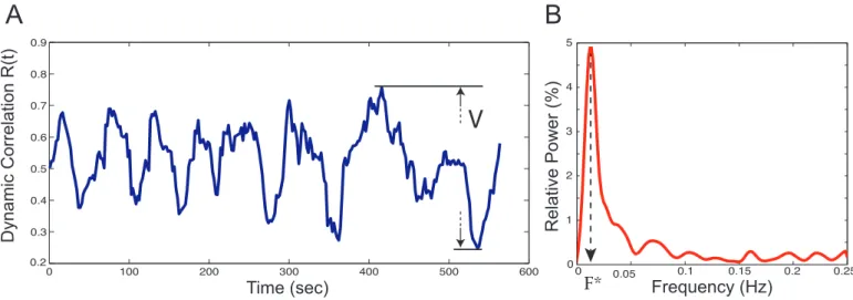
Figure 2: (A) Temporal evolution of the dynamic correlation between SC and FC. (B) Corresponding power spectrum. Results are shown for a representative subject and a window width of w = 13TR. The static correlation = 39.1%, V = 51.7% and F∗= 0.012Hz
Sliding Window for FC Analysis
In order to explore the dynamics in the correlations be-tween structural and functional connectivities we repeated the computation of the FC matrices from truncated por-tions of the fMRI time series, as previously presented (Chang and Glover, 2010; Hutchison et al., 2012; Allen et al., 2012; Leonardi et al., 2013).
Denoting by T the number of volumes in the fMRI time series and considering a window width w (the width of the truncated portions), we computed T − w + 1 successive FC matrices from the truncated fMRI time series in each particular window, each one being shifted forward by one TR with respect to the previous one (Figure 1Comparison between the static and the dynamic analysis of the cor-relation between structural and functional connectivities (SC and FC, resp.). (A) FC is computed using the whole fMRI time course. (B) dFC is computed in windows of the fMRI time courses that are slid across the whole fMRI time course. (C) Static correlation Rstaticbetween SC and FC, as computed in e.g. Honey et al. (2009). (D) Dynamic correlation Rdyn(t) between SC and FC(t), normalized by
Rstaticand used in the present workfigure.1B).
We used window widths ranging from 2 to 100 volumes, corresponding to 4 to 200 seconds, to explore the dynamics between structural and functional connectivities.
Dynamic correlation between structural and functional ma-trices
We then computed the correlation between all the FC matrices and the SC matrix (Figure 1Comparison between the static and the dynamic analysis of the correlation be-tween structural and functional connectivities (SC and FC, resp.). (A) FC is computed using the whole fMRI time course. (B) dFC is computed in windows of the fMRI time courses that are slid across the whole fMRI time course. (C) Static correlation Rstaticbetween SC and FC, as com-puted in e.g. Honey et al. (2009). (D) Dynamic
correla-tion Rdyn(t) between SC and FC(t), normalized by Rstatic and used in the present workfigure.1D). This included log-rescaling of the non-zero values in the SC matrix such that the range in both connectivity matrices have the same or-der of magnitude (see Supplementary Material for further details).
The evolution of this correlation was normalized by the static correlation between the SC and the FC matrices computed using the whole fMRI time series (Figure 1Com-parison between the static and the dynamic analysis of the correlation between structural and functional connectivi-ties (SC and FC, resp.). (A) FC is computed using the whole fMRI time course. (B) dFC is computed in win-dows of the fMRI time courses that are slid across the whole fMRI time course. (C) Static correlation Rstatic between SC and FC, as computed in e.g. Honey et al. (2009). (D) Dynamic correlation Rdyn(t) between SC and FC(t), normalized by Rstatic and used in the present workfigure.1C,D), resulting in what we call the dynamic correlation, denoted by R(t).
In order to characterize the fluctuations of the dynamic correlation the power spectrum of R(t) was computed us-ing Welch’s method (Welch, 1967) and normalized such that R0.25
0 P (f )dF = 1 where P (f ) is the power spectral content corresponding to frequency f .
Values of interest
In order to characterize dynamics observed in the time-evolving dynamic correlation curves and their correspond-ing spectral power, we used two markers:
• V is the range of variation in the dynamic correla-tion, computed as the difference between its maximal and minimal value, in percent. V is used to high-light the phases of (de)synchronization between SC and FC (Fig 2(A) Temporal evolution of the dynamic correlation between SC and FC. (B) Corresponding
power spectrum. Results are shown for a represen-tative subject and a window width of w = 13TR. The static correlation = 39.1%, V = 51.7% and F∗= 0.012Hzfigure.2A),
• F∗is the frequency of maximal relative spectral power (in Hz), and corresponds to the main oscillatory mode of a time course, such as in Figure 2(A) Tempo-ral evolution of the dynamic correlation between SC and FC. (B) Corresponding power spectrum. Results are shown for a representative subject and a window width of w = 13TR. The static correlation = 39.1%, V = 51.7% and F∗= 0.012Hzfigure.2B.
Statistical significance of the observed dynamics
A main issue in fMRI time series analyses is to dis-entangle the neuronal dynamics from noise (Handwerker et al., 2012). To this end we performed the same com-putations as the one described in Figure 1Comparison between the static and the dynamic analysis of the cor-relation between structural and functional connectivities (SC and FC, resp.). (A) FC is computed using the whole fMRI time course. (B) dFC is computed in windows of the fMRI time courses that are slid across the whole fMRI time course. (C) Static correlation Rstaticbetween SC and FC, as computed in e.g. Honey et al. (2009). (D) Dynamic correlation Rdyn(t) between SC and FC(t), normalized by
Rstatic and used in the present workfigure.1 using
surro-gate data obtained by phase randomization in the Fourier domain of the fMRI volumes (Theiler et al., 1992), similar to what is presented in Allen et al. (2012), for example (see Supplementary Material for details). Doing so leaves the static correlation unchanged because the overall co-variance structure is preserved, whereas the evolution of the dynamic correlation R(t) using windowing will be to-tally rearranged.
We observed larger fluctuations (higher V ) of R(t) in the original data compared to the surrogate data. Hence, we chose this marker to test for differences between the results obtained with ordered and phase randomized fMRI time series. For each value of window width and each subject we did 1000 permutations (see e.g. Chap 3.5 in Edgington and Onghena, 1969) and computed the z-score corresponding to the following null hypothesis:
H0= {Vord≯ Vrand}
where Vord (resp. Vrand) is the range of variation of R(t) in the original ordered (resp. surrogate) data.
The group level significance curve presented in Figure 3(A) R(t) for different window widths for a representative subject in the original dataset and one sample of the surro-gate dataset. (B) Estimation of the statistical significance region at the group level based on the range of variation V of R(t)figure.3B was computed from the z-scores of all the subjects. This technique is known as the Stouffer’s
method (Stouffer et al., 1949) , and is detailed in the Sup-plementary Material.
Graph theory metrics
In order to further characterize FC during the phases of (de)synchronization with SC, we used three common graph metrics of FC considered as a weighted undirected graph (Bullmore and Sporns, 2009). In this context, each ROI is considered as a node of the graph and the level of correlation between each two regions i and j F Ci,j is the weight of the edge connecting these two regions. Since FC is symmetric, it follows that the corresponding graph is undirected. We used the three following metrics on the whole FC matrices:
• Density is the number of total connections divided by the number of possible connections (Sporns, 2002), • Efficiency measures how ’close’ every two nodes are in
the graph. It is inversely related to the characteristic path length (Onnela et al., 2005; Rubinov and Sporns, 2010),
• Modularity quantifies to which degree a network can be subdivided into distinct groups (Newman and Gir-van, 2004).
The Brain Connectivity Toolbox (Rubinov and Sporns, 2010) was used to evaluate the value of these three markers during phases of high and low correlation between SC and F C(t). For each subject, averaged top and bottom 5% of FC(t) matrices were selected, sorted by R(t) value (see Fig-ure 4(A) Illustration of the phases of (de)synchronization between FC and SC for a representative subject based on the difference in the values of V in both cases. (B) left Average FC matrix computed by averaging the FC matrices that have the 5% lowest correlations with SC. middle Structural connectivity matrix. right Average FC matrix computed by averaging the FC matrices that have the 5% highest correlations with SCfigure.4 for more de-tails). Since density was designed for binary graphs, we binarized the FC matrices (only for this marker) using a 0.1 threshold. It should be noted that the choice of the threshold does not influence the trend observed in Figure 5Density, Efficiency and Modularity of FC averaged over the 5% lowest correlations with SC (low R - left columns) and FC averaged over the 5% highest correlations with SC (high R - right columns) for all the subjects. The group mean is represented in redfigure.5 left.
Network-level analysis
All computations above have been performed at the whole-brain level. In order to test the hypothesis that the fluctuations in R(t) can be linked to consciousness-related processes, we repeated the procedure presented in Section 2.7 in selected regions, defined by the Lausanne Atlas (Hagmann et al., 2008). We tested the fluctuations in
0 100 200 300 400 500 600 0 0.2 0.4 0.6 0.8 1 0 100 200 300 400 500 600 0 0.2 0.4 0.6 0.8 1 0 0.2 0.4 0.6 0.8 1 Time (sec) 0 100 200 300 400 500 600 0 100 200 300 400 500 600 0 0.2 0.4 0.6 0.8 1 0 100 200 300 400 500 600 0 0.2 0.4 0.6 0.8 1 0 100 200 300 400 500 600 0 0.2 0.4 0.6 0.8 1 Time (sec) Dynamic Correlation R(t) Dynamic Correlation R(t) w=4 w=4 w=13 w=13 w=50 w=50 V=72% V=71% V=38% V=53% V=32% V=34%
Ordered Case Phase randomized Case
A Single subject illustration
1 10 100 0.4 0.6 0.8 1 1.2 1.4 1.6 1.8 2
B Group-level significance
z-score Window width w Range of values ofw that best unveil dynamics of R(t)
Figure 3: (A) R(t) for different window widths for a representa-tive subject in the original dataset and one sample of the surrogate dataset. (B) Estimation of the statistical significance region at the group level based on the range of variation V of R(t)
the precuneus for the default mode network (DMN), and the supramarginal region for the cognitive control network (CCN). These two regions are known to be involved in mind-wandering processes (e.g. Fox et al., 2013). We also tested these fluctuations in two regions of the somato-motor network: the precentral gyrus for the motor network (MOT) and in the postcentral gyrus for the somatosensory network (SS).
In order to test the similarity between the effect observed at the brain level and in the four networks, we computed the correlation between the z-scores equivalent to the curves presented in Figures 3(A) R(t) for different window widths for a representative subject in the original dataset and one sample of the surrogate dataset. (B) Estimation of the statistical significance region at the group level based on the range of variation V of R(t)figure.3B and 6Right Statistical significance of fluctuations for
four different regions in four different networks. DMN: precuneus; CC: supramarginal; SS: postcentral; MOT: precentral. Correlation coefficients between the equivalent z-scores curves of the four networks and the brain-level curve presented in Figure 3(A) R(t) for different window widths for a representative subject in the original dataset and one sample of the surrogate dataset. (B) Estimation of the statistical significance region at the group level based on the range of variation V of R(t)figure.3B are represented on the curves. Left Inter-network difference of significance tests deduced from the equivalent z-scores and for w=20 TRfigure.6. This correlation coefficient is indicated next to the corresponding curve in Figure 6Right Statistical significance of fluctuations for four different regions in four different networks. DMN: precuneus; CC: supramarginal; SS: postcentral; MOT: precentral. Correlation coefficients between the equivalent z-scores curves of the four networks and the brain-level curve presented in Figure 3(A) R(t) for different window widths for a representative subject in the original dataset and one sample of the surrogate dataset. (B) Estimation of the statistical significance region at the group level based on the range of variation V of R(t)figure.3B are represented on the curves. Left Inter-network difference of significance tests deduced from the equivalent z-scores and for w=20 TRfigure.6.
Next, in order to test the difference between the effects observed in the four networks and for w = 20 TR, we performed a paired t-test using the equivalent z-scores obtained at the first step of Stouffer’s method (see Supplementary Material) for w = 20 TR. The results are represented in the table on the left of Figure 6Right Statistical significance of fluctuations for four different regions in four different networks. DMN: precuneus; CC: supramarginal; SS: postcentral; MOT: precentral. Correlation coefficients between the equivalent z-scores curves of the four networks and the brain-level curve presented in Figure 3(A) R(t) for different window widths for a representative subject in the original dataset and one sample of the surrogate dataset. (B) Estimation of the statistical significance region at the group level based on the range of variation V of R(t)figure.3B are represented on the curves. Left Inter-network difference of significance tests deduced from the equivalent z-scores and for w=20 TRfigure.6.
Results
Statistical significance of dynamical correlation
The dynamical correlation for a representative subject is shown in Figure 2(A) Temporal evolution of the dynamic correlation between SC and FC. (B) Corresponding power spectrum. Results are shown for a representative subject and a window width of w = 13TR. The static correlation = 39.1%, V = 51.7% and F∗ = 0.012Hzfigure.2 for a
window width = 13 TR. In this example the dynamic cor-relation varies from 24% to 76% (R = 52%) of the static correlation, and the peak spectral power is F∗= 0.012Hz. The choice of window width w affects the way dynam-ical correlation is captured (see Figure 8(A) R(t) and (B) corresponding power spectrum for different window widths w and for a representative subject. (C) Mean and standard deviation of F∗ for all subjects as a function of the window width wfigure.8 in Supplementary Material). Significance of observed fluctuations as a function of w is represented in Figure 3(A) R(t) for different window widths for a representative subject in the original dataset and one sample of the surrogate dataset. (B) Estimation of the statistical significance region at the group level based on the range of variation V of R(t)figure.3 and was tested by comparison against phase randomized fMRI time series as explained in the Methods section.
Figure 3(A) R(t) for different window widths for a rep-resentative subject in the original dataset and one sample of the surrogate dataset. (B) Estimation of the statistical significance region at the group level based on the range of variation V of R(t)figure.3A illustrates the fact that the difference between ordered and phase randomized fMRI time series as captured by V is more pronounced for in-termediate values of w. At the group level, a peak of statistical significance can be observed around w = 20 TR (Figure 3(A) R(t) for different window widths for a rep-resentative subject in the original dataset and one sample of the surrogate dataset. (B) Estimation of the statistical significance region at the group level based on the range of variation V of R(t)figure.3B) hence this is the window width that we will use in the following analyses.
Phases of (de)synchronization between functional and structural connectivities
We show in Figure 4(A) Illustration of the phases of (de)synchronization between FC and SC for a represen-tative subject based on the difference in the values of V in both cases. (B) left Average FC matrix computed by averaging the FC matrices that have the 5% lowest correlations with SC. middle Structural connectivity ma-trix. right Average FC matrix computed by averaging the FC matrices that have the 5% highest correlations with SCfigure.4A the statistically significant phases of (de)synchronization between FC(t) and SC, corresponding to the highest and lowest values of R(t), respectively. The average patterns of FC(t) computed during these phases are represented in Figure 4(A) Illustration of the phases of (de)synchronization between FC and SC for a represen-tative subject based on the difference in the values of V in both cases. (B) left Average FC matrix computed by aver-aging the FC matrices that have the 5% lowest correlations with SC. middle Structural connectivity matrix. right Av-erage FC matrix computed by averaging the FC matrices that have the 5% highest correlations with SCfigure.4B as
well as the constant structural connectivity matrix, for one particular subject.
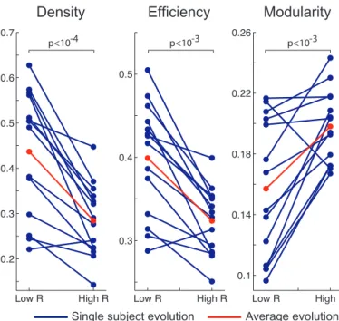
Density, efficiency and modularity of the high and low FC patterns for all the subjects are represented in Figure 5Density, Efficiency and Modularity of FC averaged over the 5% lowest correlations with SC (low R - left columns) and FC averaged over the 5% highest correlations with SC (high R - right columns) for all the subjects. The group mean is represented in redfigure.5.
Low R High R 0.2 0.3 0.4 0.5 0.6 0.7
Density
Low R High R 0.3 0.4 0.5Efficiency
Low R High R 0.1 0.14 0.18 0.22 0.26Modularity
Single subject evolution Average evolution
p<10-3
p<10-4 p<10-3
Figure 5: Density, Efficiency and Modularity of FC averaged over the 5% lowest correlations with SC (low R - left columns) and FC averaged over the 5% highest correlations with SC (high R - right columns) for all the subjects. The group mean is represented in red.
Density and efficiency appear to be significantly lower (p < 10−4 and p < 10−3 using a paired t-test) when the correlation between FC(t) and SC is high whereas modu-larity increases at the same time (p < 10−3).
Networks implied in the fluctuations
The statistical significance of the fluctuations in four different regions of the brain, representative of four net-works, are represented in Figure 6Right Statistical signifi-cance of fluctuations for four different regions in four differ-ent networks. DMN: precuneus; CC: supramarginal; SS: postcentral; MOT: precentral. Correlation coefficients be-tween the equivalent z-scores curves of the four networks and the brain-level curve presented in Figure 3(A) R(t) for different window widths for a representative subject in the original dataset and one sample of the surrogate dataset. (B) Estimation of the statistical significance re-gion at the group level based on the range of variation V of R(t)figure.3B are represented on the curves. Left Inter-network difference of significance tests deduced from the equivalent z-scores and for w=20 TRfigure.6.
0 100 200 300 400 500 600 0.2 0.3 0.4 0.5 0.6 0.7 0.8 0.9 0 100 200 300 400 500 600 0.2 0.3 0.4 0.5 0.6 0.7 0.8 0.9
Relative Correlation Relative Correlation
Ordered case (R=51.7%) Phase randomized case (R=28.6%)
Phases of statistically significant low correlation Phases of statistically significant high correlation
R
Time (sec) Time (sec)
-0.8 -0.6 -0.4 -0.2 0 0.2 0.4 0.6 0.8 1 AUD SM VIS CC DM 0 1 2 3 4 5 6 7 -0.6 -0.4 -0.2 0 0.2 0.4 0.6 0.8 1 AUD SM VIS CC DM AUD SM VIS CC DM
A
B
Average FC during SC Average FC during
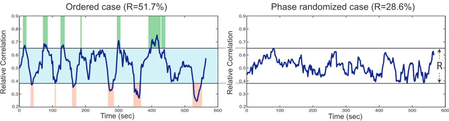
Figure 4: (A) Illustration of the phases of (de)synchronization between FC and SC for a representative subject based on the difference in the values of V in both cases. (B) left Average FC matrix computed by averaging the FC matrices that have the 5% lowest correlations with SC. middle Structural connectivity matrix. right Average FC matrix computed by averaging the FC matrices that have the 5% highest correlations with SC.
The characteristic ’V’ shape observed at the whole-brain level in Figure 3(A) R(t) for different window widths for a representative subject in the original dataset and one sample of the surrogate dataset. (B) Estimation of the statistical significance region at the group level based on the range of variation V of R(t)figure.3B is present in the DMN and the CC but not in the MOT and SS networks, as indicated by the correlation coefficients between the equiv-alent z-scores curves (see Methods section). In addition, the significance of the fluctuations appears to be lower in the DMN and the CCN compared to the SS and MOT networks as shown by the p-values in the table on the left of Figure 6Right Statistical significance of fluctuations for four different regions in four different networks. DMN: cuneus; CC: supramarginal; SS: postcentral; MOT: pre-central. Correlation coefficients between the equivalent z-scores curves of the four networks and the brain-level curve presented in Figure 3(A) R(t) for different window widths
for a representative subject in the original dataset and one sample of the surrogate dataset. (B) Estimation of the sta-tistical significance region at the group level based on the range of variation V of R(t)figure.3B are represented on the curves. Left Inter-network difference of significance tests deduced from the equivalent z-scores and for w=20 TRfigure.6.
Discussion
A) Significance of fluctuations observed using the sliding window approach
Sliding window techniques have been widely used in re-cent studies in order to analyze FC dynamics. Allen et al. (2012) used a width of 22 TR (TR=2 sec) to track oscil-lations in FC dynamics, Shirer et al. (2012) showed that considering a width above 15-30 TR (TR=2 sec) allows for robust estimates of the FC without considering dynamics.
Statistical difference between signifi-cance in networks for w = 20TR CC DM SS MOT CC DM SS MOT .22 .013 .017 .22 .020 .021 .013 .020 .43 .017 .021 .43 1 10 100 -0.2 0 0.2 0.4 0.6 0.8 1 1.2
Cognitive Control Network Motor Network Somato Sensory Network Default Mode Network
Group-level z-score in four networks
Window width w
0.85 0.88
0.66
0.69
Figure 6: Right Statistical significance of fluctuations for four differ-ent regions in four differdiffer-ent networks. DMN: precuneus; CC: supra-marginal; SS: postcentral; MOT: precentral. Correlation coefficients between the equivalent z-scores curves of the four networks and the brain-level curve presented in Figure 3(A) R(t) for different window widths for a representative subject in the original dataset and one sample of the surrogate dataset. (B) Estimation of the statistical significance region at the group level based on the range of variation V of R(t)figure.3B are represented on the curves. Left Inter-network difference of significance tests deduced from the equivalent z-scores and for w=20 TR.
More recently, Leonardi et al. (2013) used widths rang-ing from 20 to 120 TR (TR=1.1 sec) and observed differ-ent “eigenconnectivity patterns” depending on the window that is used and Hutchison et al. (2012) also found differ-ent results with window width going from 10 to 120 TR (TR=2 sec).
Our study reveals a peak of statistical significance in the observed fluctuations around w = 20 − 30 TR (TR=2 sec). This peak is observed using the range of variation V of R(t). Another statistical test based on the variance of the R(t) curves (see Figure 9Estimation of the statistical significance region based on the variance of the dynamic correlation R(t)figure.9 in Supplementary Material) also shows a peak for values of w around 20 TR which rein-forces our conclusions about which window width should be used.
Our results are consistent with a general tradeoff in time series analyses: longer windows improve the estimation of the correlation but mask the dynamics because they act as low-pass filters. This effect is illustrated by the green curve in Figure 7Interpretation of Figure 3(A) R(t) for different window widths for a representative subject in the original dataset and one sample of the surrogate dataset. (B) Estimation of the statistical significance re-gion at the group level based on the range of variation V of R(t)figure.3: tradeoff between capturing dynamics and estimating correlationfigure.7 and was studied by Shirer et al. (2012).
Our analysis provides the additional insight that con-sidering higher values of w does not capture the FC neu-ronal dynamics, which is illustrated by the red curve in Figure 7Interpretation of Figure 3(A) R(t) for different
Large Small Window width (w) St a ti st ica l Si g n if ica n ce 1 0 Estimatin g Correlation Capturing Dynamics Region of globally higher statistical significance (high z-score)
Figure 7: Interpretation of Figure 3(A) R(t) for different window widths for a representative subject in the original dataset and one sample of the surrogate dataset. (B) Estimation of the statistical sig-nificance region at the group level based on the range of variation V of R(t)figure.3: tradeoff between capturing dynamics and estimating correlation
window widths for a representative subject in the orig-inal dataset and one sample of the surrogate dataset. (B) Estimation of the statistical significance region at the group level based on the range of variation V of R(t)figure.3: tradeoff between capturing dynamics and es-timating correlationfigure.7. Indeed, we can compare win-dowing of correlations to a moving average which is a low-pass filter with cutoff frequency fcthat decreases when w increases (e.g. Smith, 1997, Chap.15).
We hereby also want to stress the importance of assessing the neuronal origin of fluctuations that are observed in dynamic functional connectivity (Hutchison et al., 2013). The simple significance testing framework proposed in the present work is believed to be an important prerequisite to further interpretation of observed functional connectivity fluctuations.
Limitations
The sliding window acts as a low-pass filter. In our case, considering w = 20 TR = 40 sec results in a cutoff frequency fc≈ 0.02 Hz. Hence, a robust estimation of FC, which requires a window width w ≈ 20 TR, necessarily fil-ters out the FC dynamics happening at higher frequencies than ≈ 0.02 Hz.
This limitation should be taken into account when inter-preting results of dynamical FC analyses using sliding win-dows. This is also a call for more advanced identification methods that could better estimate the FC and push the green curve of Figure 7Interpretation of Figure 3(A) R(t) for different window widths for a representative subject in the original dataset and one sample of the surrogate dataset. (B) Estimation of the statistical significance re-gion at the group level based on the range of variation V of R(t)figure.3: tradeoff between capturing dynamics and estimating correlationfigure.7 to the left, consequently freeing the access to higher frequency dynamics.
B) Phases of (de)synchronization between functional and structural connectivities
The link between structural and functional connectivi-ties was established a few years ago (Honey et al., 2009; van den Heuvel et al., 2009). Thereafter, a lot of in-terest has been devoted to deepen the understanding of how anatomical constraints shape functional connectivity (Honey et al., 2010; Breakspear et al., 2010; Cabral et al., 2011; Deco et al., 2012), and how this relationship can be affected by different pathologies (de Kwaasteniet et al., 2013; van Schouwenburg et al., 2013).
In most of these studies either the dynamics of FC are not taken into account, or it is modeled, but the information coming from the data and used to assess models is deduced with a static approach of FC (e.g. Deco et al., 2013b). To our knowledge, our paper is the first data driven at-tempt to study the dynamical relationship between SC and FC. More specifically, we show in Figure 3(A) R(t) for different window widths for a representative subject in the original dataset and one sample of the surrogate dataset. (B) Estimation of the statistical significance re-gion at the group level based on the range of variation V of R(t)figure.3 that there are statistically significant (i.e. resulting from the neuronal dynamics, not noise) phases of (de)synchronization between the functional correlation and the anatomical constraints. When using statistically significant values of w such as w = 20 TR, the range of variation R is on the order of 52% of the static correla-tion, compared to 34% in the randomized case, meaning that the correlation between FC and SC is significantly high at some points and significantly low at some other points.
Structure as a switch between functional brain states Diverse studies have recently highlighted the presence of different and successive functional connectivity states, even at rest (Lv et al., 2013; Gao et al., 2010; Deco et al., 2013a; Yang et al., 2014; Sidlauskaite et al., 2014). The results shown in Figures 4(A) Illustration of the phases of (de)synchronization between FC and SC for a repre-sentative subject based on the difference in the values of V in both cases. (B) left Average FC matrix computed by averaging the FC matrices that have the 5% lowest correlations with SC. middle Structural connectivity matrix. right Average FC matrix computed by averaging the FC matrices that have the 5% highest correlations with SCfigure.4 and 5Density, Efficiency and Modularity of FC averaged over the 5% lowest correlations with SC (low R - left columns) and FC averaged over the 5% highest correlations with SC (high R - right columns) for all the subjects. The group mean is represented in redfigure.5 suggest that the dynamic reorganization of functional connectivity patterns is shaped by anatomy. More particularly it can be observed from Figure 5Den-sity, Efficiency and Modularity of FC averaged over the 5% lowest correlations with SC (low R - left columns) and
FC averaged over the 5% highest correlations with SC (high R - right columns) for all the subjects. The group mean is represented in redfigure.5 that phases of high correlation between FC and SC correspond to functional connectivity patterns that have poor efficiency and high modularity. The interpretation is that during these phases the brain is poorly functionally connected, and organized in modules shaped by anatomy with few inter-modules connections (Newman and Girvan, 2004). On the other hand, during phases of low correlation between FC and SC, the number of inter-modules functional connections increases, resulting in highly connected FC patterns. Very recently, Mess´e et al. (2014) evinced a decoupling between anatomy-defined networks and other networks resulting from stationary and non-stationary FC dynam-ics, but not related to anatomy. Combined to our results, these observations lead us to propose that anatomy could periodically play the role of a relay that guides switches between different highly connected FC patterns not shaped by anatomy (red regions in Figure 4(A) Illustra-tion of the phases of (de)synchronizaIllustra-tion between FC and SC for a representative subject based on the difference in the values of V in both cases. (B) left Average FC matrix computed by averaging the FC matrices that have the 5% lowest correlations with SC. middle Structural connectivity matrix. right Average FC matrix computed by averaging the FC matrices that have the 5% highest correlations with SCfigure.4A), alternating with phases of lower efficiency and higher modularity, defined by SC architecture (green regions in Figure 4(A) Illustration of the phases of (de)synchronization between FC and SC for a representative subject based on the difference in the values of V in both cases. (B) left Average FC matrix computed by averaging the FC matrices that have the 5% lowest correlations with SC. middle Structural connectivity matrix. right Average FC matrix computed by averaging the FC matrices that have the 5% highest correlations with SCfigure.4A). This interpretation echoes another recent work (Zalesky et al., 2014) in which the most dynamic connections are shown to be inter-modular, and support the emergence of temporary phases of high functional efficiency.
R(t) as a foot-print of mind-wandering
The strength of the link between anatomy and func-tional correlates has been shown to vary between differ-ent attdiffer-entional states (Baria et al., 2013). Several of our results provide temporal and spatial indicators of the sta-tistical correlation between R(t) and mind-wandering pro-cesses. First, we showed that the fluctuations of R(t) are statistically significant when a window width in the range 20 − 30 TR is used, corresponding to a main oscillatory mode F∗on the order of 0.01 ± 0.003 Hz (Figure 8(A) R(t) and (B) corresponding power spectrum for different win-dow widths w and for a representative subject. (C) Mean and standard deviation of F∗for all subjects as a function
of the window width wfigure.8C in Supplementary Ma-terial), which is quite close to the typical frequencies of networks mediating consciousness markers such as aware-ness of environment and of self (Vanhaudenhuyse et al., 2011). Second, the results presented in Figure 6Right Sta-tistical significance of fluctuations for four different regions in four different networks. DMN: precuneus; CC: supra-marginal; SS: postcentral; MOT: precentral. Correlation coefficients between the equivalent z-scores curves of the four networks and the brain-level curve presented in Fig-ure 3(A) R(t) for different window widths for a representa-tive subject in the original dataset and one sample of the surrogate dataset. (B) Estimation of the statistical sig-nificance region at the group level based on the range of variation V of R(t)figure.3B are represented on the curves. Left Inter-network difference of significance tests deduced from the equivalent z-scores and for w=20 TRfigure.6 show that the significance curves for DM and CC present the characteristic ’V’ shape that is found at the brain level, whereas the curves in the MOT and SS networks are al-most flat resulting in lower correlation coefficients for these networks. In addition, the level of significance appears to be significantly higher in the DMN and the CC compared to the other two networks (Figure 6Right Statistical sig-nificance of fluctuations for four different regions in four different networks. DMN: precuneus; CC: supramarginal; SS: postcentral; MOT: precentral. Correlation coefficients between the equivalent z-scores curves of the four networks and the brain-level curve presented in Figure 3(A) R(t) for different window widths for a representative subject in the original dataset and one sample of the surrogate dataset. (B) Estimation of the statistical significance re-gion at the group level based on the range of variation V of R(t)figure.3B are represented on the curves. Left Inter-network difference of significance tests deduced from the equivalent z-scores and for w=20 TRfigure.6(left), tested for w=20 TR). This suggests that the fluctuations that are observed in R(t) are driven by neuronal dynamics happen-ing in the DM and CC networks and not in the MOT and SS networks and are consequently at least partly corre-lated to mind-wandering effects.
Going further, Doucet et al. (2012) reported that mind-wandering was correlated with fluctuations of functional modular organization, inner-oriented activities being as-sociated to phases of low inter-modular connectivity. This is an additional evidence supporting the interpretation of R(t) as reflecting mind-wandering processes.
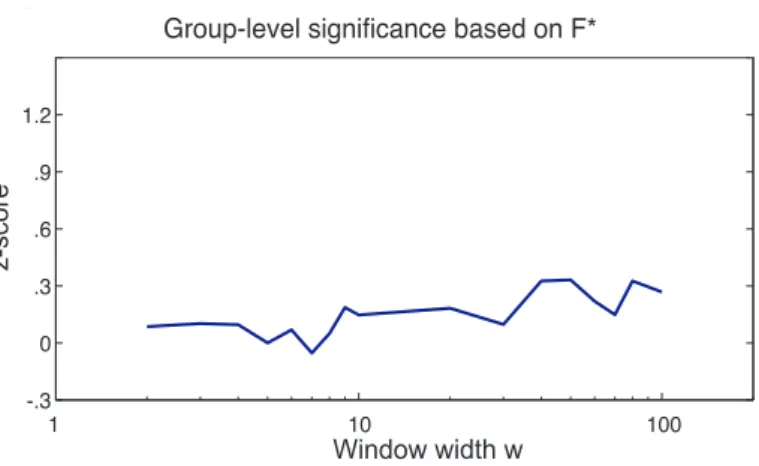
Limitations
We use F∗to characterize the fluctuations of R(t). It is interesting to note that we were not able to distinguish or-dered from phase randomized time courses using F∗ (see Figure 10Estimation of the statistical significance region based on F∗figure.10 in the Supplementary Material), sug-gesting that F∗ is imposed by the sliding window method and by w (Figure 8(A) R(t) and (B) corresponding power spectrum for different window widths w and for a
represen-tative subject. (C) Mean and standard deviation of F∗for all subjects as a function of the window width wfigure.8C in the Supplementary Material) and is not a priori cap-turing neuronal dynamics. Hence it is not surprising to find similar values of F∗in studies using a similar window width: Allen et al. (2012) found oscillations at 0.005-0.015 Hz using a 22 TR (44 sec) windowing. However, as ar-gued in Hutchison et al. (2013), this does not imply that the value of F∗ for ordered fMRI time series has a non-neuronal origin. It is used here because the significance of oscillations was independently assessed using two other markers of R(t).
Finally it should be highlighted that having a frequency peak at around 0.01 Hz for the values of w that are sta-tistically significant does not mean that the dynamics are only occurring at these frequencies. As explained earlier, hypothetical dynamics happening at higher frequencies are filtered out when we use 20 TR windowing and it is, for example, difficult to assess the correspondence with the consciousness markers from a dynamical point of view be-cause they are happening at higher frequencies.
C) Future work
The results of this paper call for several methodologi-cal refinements. We have presented a hypothesis-driven approach in order to test which network contributes most strongly to the bralevel oscillations. It would be in-teresting to use data-driven approaches in order to finely identify which areas contribute more strongly to the over-all fluctuations of R(t). Addressing this problem requires a solution for the dimensionality issues raised in this ap-plication. Indeed, if one wants to derive networks without needing any a priori knowledge, we would have either to use adequate downscaling or to consider every pair of vox-els as a variable, that is O(N2) variables where N is the number of ROIs, 1015 in our case.
Moreover, windowing is an approach that shows some limi-tations, and future studies should consider more advanced techniques for the dynamics identification. These alter-natives may allow for clearer identification of dynamics of functional connectivity, and could help unveil processes oc-curring at higher frequencies such as mind-wandering. As fast scanning becomes feasible with new scanners and par-allel imaging, one simple way to test this hypothesis would be to use smaller TRs, up to 1 sec, in order to increase the lowpass cutoff frequency of the windowing process. It could also be worth completing the present multi-modal analysis with other imaging modalities such as EEG. It has, for example, been shown that EEG micro-states can be considered as building blocks of cognition and shape fMRI networks (Van de Ville et al., 2010). Hence, includ-ing the high-resolution temporal information provided by EEG measurements could lead to a better understanding of the interaction between anatomy and function and its interpretation in terms of cognitive processes.
Conclusions
The contribution of the present paper is twofold. From a methodological point of view we highlight some character-istics of the sliding window technique to reveal functional connectivity dynamics. Our results suggest that the width of those windows should be chosen around the 20-30 TR (40-60 sec) range to both provide a robust estimate of the correlation and capture significant functional connectiv-ity neuronal dynamics. For smaller or higher values, we could not significantly distinguish functional connectivity dynamics from noise with similar properties.
Next, we use a suitable window width to show that that dynamical functional connectivity oscillates between states of high modularity, mostly shaped by structural connec-tivity architecture, and states of low modularity, not de-fined by structural connectivity, during which more inter-network connections take place.
Finally, considering that these fluctuations are occuring at a characteristic frequency of ≈ 0.01 Hz and that the De-fault Mode and the Cognitive Control networks are highly contributing to their dynamics, we propose that the dy-namical correlation between functional connectivity and anatomy is an interesting marker of mind-wandering ef-fects.
References
Allen, E.A., Damaraju, E., Plis, S.M., Erhardt, E.B., Eichele, T., Calhoun, V.D., 2012. Tracking whole-brain connectivity dynamics in the resting state. Cereb Cortex .
Amico, E., Gomez, F., Di Perri, C., Vanhaudenhuyse, A., Lesenfants, D., Boveroux, P., Bonhomme, V., Brichant, J.F., Marinazzo, D., Laureys, S., 2014. Posterior cingulate cortex-related co-activation patterns: a resting state fmri study in propofol-induced loss of consciousness. PLoS One 9, e100012.
Baria, A.T., Mansour, A., Huang, L., Baliki, M.N., Cecchi, G.A., Mesulam, M.M., Apkarian, A.V., 2013. Linking human brain lo-cal activity fluctuations to structural and functional network ar-chitectures. Neuroimage 73, 144–55.
Bassett, D.S., Wymbs, N.F., Porter, M.A., Mucha, P.J., Carlson, J.M., Grafton, S.T., 2011. Dynamic reconfiguration of human brain networks during learning. Proc Natl Acad Sci U S A 108, 7641–6.
Bastian, M., Sackur, J., 2013. Mind wandering at the fingertips: au-tomatic parsing of subjective states based on response time vari-ability. Front Psychol 4, 573.
Beckmann, C.F., DeLuca, M., Devlin, J.T., Smith, S.M., 2005. Inves-tigations into resting-state connectivity using independent compo-nent analysis. Philos Trans R Soc Lond B Biol Sci 360, 1001–13. Breakspear, M., Jirsa, V., Deco, G., 2010. Computational models of
the brain: from structure to function. Neuroimage 52, 727–30. Bullmore, E., Sporns, O., 2009. Complex brain networks: graph
theoretical analysis of structural and functional systems. Nat Rev Neurosci 10, 186–98.
Cabral, J., Hugues, E., Sporns, O., Deco, G., 2011. Role of local network oscillations in resting-state functional connectivity. Neu-roimage 57, 130–9.
Cammoun, L., Gigandet, X., Meskaldji, D., Thiran, J.P., Sporns, O., Do, K.Q., Maeder, P., Meuli, R., Hagmann, P., 2012. Mapping the human connectome at multiple scales with diffusion spectrum mri. J Neurosci Methods 203, 386–97.
Chang, C., Glover, G.H., 2010. Time-frequency dynamics of resting-state brain connectivity measured with fmri. Neuroimage 50, 81–98.
Christoff, K., Gordon, A.M., Smallwood, J., Smith, R., Schooler, J.W., 2009. Experience sampling during fmri reveals default net-work and executive system contributions to mind wandering. Proc Natl Acad Sci U S A 106, 8719–24.
Damoiseaux, J.S., Greicius, M.D., 2009. Greater than the sum of its parts: a review of studies combining structural connectivity and resting-state functional connectivity. Brain Struct Funct 213, 525–33.
Damoiseaux, J.S., Rombouts, S.A.R.B., Barkhof, F., Scheltens, P., Stam, C.J., Smith, S.M., Beckmann, C.F., 2006. Consistent resting-state networks across healthy subjects. Proc Natl Acad Sci U S A 103, 13848–53.
Deco, G., Hagmann, P., Hudetz, A.G., Tononi, G., 2013a. Modeling resting-state functional networks when the cortex falls sleep: Local and global changes. Cereb Cortex .
Deco, G., Ponce-Alvarez, A., Mantini, D., Romani, G.L., Hagmann, P., Corbetta, M., 2013b. Resting-state functional connectivity emerges from structurally and dynamically shaped slow linear fluctuations. J Neurosci 33, 11239–52.
Deco, G., Senden, M., Jirsa, V., 2012. How anatomy shapes dynam-ics: a semi-analytical study of the brain at rest by a simple spin model. Front Comput Neurosci 6, 68.
Desikan, R.S., S´egonne, F., Fischl, B., Quinn, B.T., Dickerson, B.C., Blacker, D., Buckner, R.L., Dale, A.M., Maguire, R.P., Hyman, B.T., Albert, M.S., Killiany, R.J., 2006. An automated labeling system for subdividing the human cerebral cortex on mri scans into gyral based regions of interest. Neuroimage 31, 968–80. Doucet, G., Naveau, M., Petit, L., Zago, L., Crivello, F., Jobard, G.,
Delcroix, N., Mellet, E., Tzourio-Mazoyer, N., Mazoyer, B., Joliot, M., 2012. Patterns of hemodynamic low-frequency oscillations in the brain are modulated by the nature of free thought during rest. Neuroimage 59, 3194–200.
Edgington, E., Onghena, P., 1969. Randomization Tests. CRC Press. Engel, Jr, J., Thompson, P.M., Stern, J.M., Staba, R.J., Bragin, A., Mody, I., 2013. Connectomics and epilepsy. Curr Opin Neurol 26, 186–94.
Eryilmaz, H., Van De Ville, D., Schwartz, S., Vuilleumier, P., 2011. Impact of transient emotions on functional connectivity during subsequent resting state: a wavelet correlation approach. Neu-roimage 54, 2481–91.
Fox, K.C.R., Nijeboer, S., Solomonova, E., Domhoff, G.W., Christoff, K., 2013. Dreaming as mind wandering: evidence from functional neuroimaging and first-person content reports. Front Hum Neurosci 7, 412.
Friston, K.J., 2011. Functional and effective connectivity: a review. Brain Connectivity 1, 13–36.
Gao, W., Zhu, H., Giovanello, K., Lin, W., 2010. Multivariate network-level approach to detect interactions between large-scale functional systems. Med Image Comput Comput Assist Interv 13, 298–305.
Gorgolewski, K., Burns, C.D., Madison, C., Clark, D., Halchenko, Y.O., Waskom, M.L., Ghosh, S.S., 2011. Nipype: a flexible, lightweight and extensible neuroimaging data processing frame-work in python. Front Neuroinform 5, 13.
Greicius, M.D., Krasnow, B., Reiss, A.L., Menon, V., 2003. Func-tional connectivity in the resting brain: a network analysis of the default mode hypothesis. Proc Natl Acad Sci U S A 100, 253–8. Griffa, A., Baumann, P.S., Thiran, J.P., Hagmann, P., 2013.
Struc-tural connectomics in brain diseases. Neuroimage 80, 515–26. Gusnard, D.A., Raichle, M.E., Raichle, M.E., 2001. Searching for a
baseline: functional imaging and the resting human brain. Nat Rev Neurosci 2, 685–94.
Hagmann, P., Cammoun, L., Gigandet, X., Meuli, R., Honey, C.J., Wedeen, V.J., Sporns, O., 2008. Mapping the structural core of human cerebral cortex. PLoS Biol 6, e159.
Handwerker, D.A., Roopchansingh, V., Gonzalez-Castillo, J., Ban-dettini, P.A., 2012. Periodic changes in fmri connectivity. Neu-roimage 63, 1712–9.
Hasenkamp, W., Wilson-Mendenhall, C.D., Duncan, E., Barsalou, L.W., 2012. Mind wandering and attention during focused med-itation: a fine-grained temporal analysis of fluctuating cognitive
states. Neuroimage 59, 750–60.
Heine, L., Soddu, A., G´omez, F., Vanhaudenhuyse, A., Tshibanda, L., Thonnard, M., Charland-Verville, V., Kirsch, M., Laureys, S., Demertzi, A., 2012. Resting state networks and consciousness: alterations of multiple resting state network connectivity in phys-iological, pharmacological, and pathological consciousness states. Front Psychol 3, 295.
van den Heuvel, M.P., Mandl, R.C.W., Kahn, R.S., Hulshoff Pol, H.E., 2009. Functionally linked resting-state networks reflect the underlying structural connectivity architecture of the human brain. Hum Brain Mapp 30, 3127–41.
Honey, C.J., Sporns, O., Cammoun, L., Gigandet, X., Thiran, J.P., Meuli, R., Hagmann, P., 2009. Predicting human resting-state functional connectivity from structural connectivity. Proc Natl Acad Sci U S A 106, 2035–40.
Honey, C.J., Thivierge, J.P., Sporns, O., 2010. Can structure predict function in the human brain? NeuroImage 52, 766–76.
Hutchison, R.M., Womelsdorf, T., Allen, E.A., Bandettini, P.A., Calhoun, V.D., Corbetta, M., Della Penna, S., Duyn, J.H., Glover, G.H., Gonzalez-Castillo, J., Handwerker, D.A., Keilholz, S., Kiviniemi, V., Leopold, D.A., de Pasquale, F., Sporns, O., Walter, M., Chang, C., 2013. Dynamic functional connectivity: Promise, issues, and interpretations. Neuroimage 80, 360–78. Hutchison, R.M., Womelsdorf, T., Gati, J.S., Everling, S., Menon,
R.S., 2012. Resting-state networks show dynamic functional con-nectivity in awake humans and anesthetized macaques. Hum Brain Mapp .
Jahanshad, N., Rajagopalan, P., Hua, X., Hibar, D.P., Nir, T.M., Toga, A.W., Jack, Jr, C.R., Saykin, A.J., Green, R.C., Weiner, M.W., Medland, S.E., Montgomery, G.W., Hansell, N.K., McMa-hon, K.L., de Zubicaray, G.I., Martin, N.G., Wright, M.J., Thompson, P.M., Alzheimer’s Disease Neuroimaging Initiative, 2013. Genome-wide scan of healthy human connectome discov-ers spon1 gene variant influencing dementia severity. Proc Natl Acad Sci U S A 110, 4768–73.
Jones, D.T., Vemuri, P., Murphy, M.C., Gunter, J.L., Senjem, M.L., Machulda, M.M., Przybelski, S.A., Gregg, B.E., Kantarci, K., Knopman, D.S., Boeve, B.F., Petersen, R.C., Jack, Jr, C.R., 2012. Non-stationarity in the ”resting brain’s” modular architecture. PLoS One 7, e39731.
Kaiser, M., 2013. The potential of the human connectome as a biomarker of brain disease. Front Hum Neurosci 7, 484.
Kiviniemi, V., Vire, T., Remes, J., Elseoud, A.A., Starck, T., Ter-vonen, O., Nikkinen, J., 2011. A sliding time-window ica reveals spatial variability of the default mode network in time. Brain Connect 1, 339–47.
Koch, M.A., Norris, D.G., Hund-Georgiadis, M., 2002. An investi-gation of functional and anatomical connectivity using magnetic resonance imaging. Neuroimage 16, 241–50.
K¨otter, R., Sommer, F.T., 2000. Global relationship between anatomical connectivity and activity propagation in the cerebral cortex. Philos Trans R Soc Lond B Biol Sci 355, 127–34. Kucyi, A., Davis, K.D., 2014. Dynamic functional connectivity of
the default mode network tracks daydreaming. Neuroimage . de Kwaasteniet, B., Ruhe, E., Caan, M., Rive, M., Olabarriaga, S.,
Groefsema, M., Heesink, L., van Wingen, G., Denys, D., 2013. Relation between structural and functional connectivity in major depressive disorder. Biol Psychiatry 74, 40–7.
Leonardi, N., Richiardi, J., Gschwind, M., Simioni, S., Annoni, J.M., Schluep, M., Vuilleumier, P., Van De Ville, D., 2013. Principal components of functional connectivity: A new approach to study dynamic brain connectivity during rest. Neuroimage .
Liu, X., Duyn, J.H., 2013. Time-varying functional network informa-tion extracted from brief instances of spontaneous brain activity. Proc Natl Acad Sci U S A 110, 4392–7.
Lv, P., Guo, L., Hu, X., Li, X., Jin, C., Han, J., Li, L., Liu, T., 2013. Modeling dynamic functional information flows on large-scale brain networks. Med Image Comput Comput Assist Interv 16, 698–705.
Macey, P.M., Macey, K.E., Kumar, R., Harper, R.M., 2004. A method for removal of global effects from fmri time series.
Neu-roImage 22, 360–6.
McIntosh, A.R., Gonzalez-Lima, F., 1994. Structural equation mod-eling and its application to network analysis in functional brain imaging. Human Brain Mapping 2, 2–22+.
Mess´e, A., Rudrauf, D., Benali, H., Marrelec, G., 2014. Relating structure and function in the human brain: relative contributions of anatomy, stationary dynamics, and non-stationarities. PLoS Comput Biol 10, e1003530.
Moussa, M.N., Steen, M.R., Laurienti, P.J., Hayasaka, S., 2012. Con-sistency of network modules in resting-state fmri connectome data. PLoS One 7, e44428.
Murphy, K., Birn, R.M., Handwerker, D.A., Jones, T.B., Bandettini, P.A., 2009. The impact of global signal regression on resting state correlations: are anti-correlated networks introduced? NeuroIm-age 44, 893–905.
Newman, M.E.J., Girvan, M., 2004. Finding and evaluating commu-nity structure in networks. Physical Review E 69, 026113+. Onnela, J.P., Saram¨aki, J., Kertesz, J., Kaski, K., 2005. Intensity
and coherence of motifs in weighted complex networks. Physical Review E 71.
Park, H.J., Friston, K., 2013. Structural and functional brain net-works: from connections to cognition. Science 342, 1238411. Passingham, R.E., Stephan, K.E., K¨otter, R., 2002. The anatomical
basis of functional localization in the cortex. Nat Rev Neurosci 3, 606–16.
Richiardi, J., Eryilmaz, H., Schwartz, S., Vuilleumier, P., Van De Ville, D., 2011. Decoding brain states from fmri connectiv-ity graphs. Neuroimage 56, 616–26.
Rubinov, M., Sporns, O., 2010. Complex network measures of brain connectivity: uses and interpretations. Neuroimage 52, 1059–69. Sako˘glu, U., Pearlson, G.D., Kiehl, K.A., Wang, Y.M., Michael, A.M., Calhoun, V.D., 2010. A method for evaluating dynamic functional network connectivity and task-modulation: application to schizophrenia. MAGMA 23, 351–66.
van Schouwenburg, M.R., Zwiers, M.P., van der Schaaf, M.E., Geurts, D.E.M., Schellekens, A.F.A., Buitelaar, J.K., Verkes, R.J., Cools, R., 2013. Anatomical connection strength predicts dopaminergic drug effects on fronto-striatal function. Psychophar-macology (Berl) 227, 521–31.
Shirer, W.R., Ryali, S., Rykhlevskaia, E., Menon, V., Greicius, M.D., 2012. Decoding subject-driven cognitive states with whole-brain connectivity patterns. Cereb Cortex 22, 158–65.
Sidlauskaite, J., Wiersema, J.R., Roeyers, H., Krebs, R.M., Vassena, E., Fias, W., Brass, M., Achten, E., Sonuga-Barke, E., 2014. An-ticipatory processes in brain state switching - evidence from a novel cued-switching task implicating default mode and salience networks. Neuroimage 98C, 359–365.
Smith, S.M., Jenkinson, M., Woolrich, M.W., Beckmann, C.F., Behrens, T.E.J., Johansen-Berg, H., Bannister, P.R., De Luca, M., Drobnjak, I., Flitney, D.E., Niazy, R.K., Saunders, J., Vick-ers, J., Zhang, Y., De Stefano, N., Brady, J.M., Matthews, P.M., 2004. Advances in functional and structural mr image analysis and implementation as fsl. Neuroimage 23 Suppl 1, S208–19. Smith, S.W., 1997. The scientist and engineer’s guide to digital signal
processing. First ed., California Technical Pub.
Sporns, O., 2002. Graph theory methods for the analysis of neural connectivity patterns. Neuroscience Databases. A Practical Guide (K¨otter, R. ed.) , 171–186.
Sporns, O., Chialvo, D., Kaiser, M., Hilgetag, C., 2004. Organiza-tion, development and function of complex brain networks. Trends in Cognitive Sciences 8, 418–425.
Sporns, O., Tononi, G., Edelman, G.M., 2000. Theoretical neu-roanatomy: relating anatomical and functional connectivity in graphs and cortical connection matrices. Cerebral Cortex 10, 127–141.
Sporns, O., Tononi, G., K¨otter, R., 2005. The human connectome: A structural description of the human brain. PLoS Comput Biol 1, e42.
Stouffer, S.E.S., DeVinney, L., Star, S., Williams, R., 1949. The american soldier, vol.1: Adjustment during army life. Princeton University Press .
Tagliazucchi, E., Balenzuela, P., Fraiman, D., Chialvo, D.R., 2012. Criticality in large-scale brain fmri dynamics unveiled by a novel point process analysis. Front Physiol 3, 15.
Theiler, J., Eubank, S., Longtin, A., Galdrikian, B., Farmer, J., 1992. Testing for nonlinearity in time series: the method of surrogate data. Physica D 58, 77–94.
Tournier, J.D., Calamante, F., Connelly, A., 2007. Robust deter-mination of the fibre orientation distribution in diffusion mri: non-negativity constrained super-resolved spherical deconvolu-tion. Neuroimage 35, 1459–72.
Tournier, J.D., Calamante, F., Gadian, D.G., Connelly, A., 2004. Direct estimation of the fiber orientation density function from diffusion-weighted mri data using spherical deconvolution. Neu-roimage 23, 1176–85.
Vanhaudenhuyse, A., Demertzi, A., Schabus, M., Noirhomme, Q., Bredart, S., Boly, M., Phillips, C., Soddu, A., Luxen, A., Moonen, G., Laureys, S., 2011. Two distinct neuronal networks mediate the awareness of environment and of self. J Cogn Neurosci 23, 570–8. Van de Ville, D., Britz, J., Michel, C.M., 2010. Eeg microstate sequences in healthy humans at rest reveal scale-free dynamics. Proc Natl Acad Sci U S A 107, 18179–84.
Welch, P.D., 1967. The use of fast fourier transform for the estima-tion of power spectra: A method based on time averaging over short, modified periodograms. Audio and Electroacoustics, IEEE Transactions on 15, 70–73.
Yang, Z., Craddock, R.C., Margulies, D.S., Yan, C.G., Milham, M.P., 2014. Common intrinsic connectivity states among posteromedial cortex subdivisions: Insights from analysis of temporal dynamics. Neuroimage 93 Pt 1, 124–37.
Zalesky, A., Fornito, A., Cocchi, L., Gollo, L.L., Breakspear, M., 2014. Time-resolved resting-state brain networks. Proc Natl Acad Sci U S A 111, 10341–6.
Ziegler, E., Foret, A., Mascetti, L., Muto, V., Le Bourdiec-Shaffii, A., Stender, J., Balteau, E., Dideberg, V., Bours, V., Maquet, P., Phillips, C., 2013. Altered white matter architecture in bdnf met carriers. PLoS One 8, e69290.
Supplementary Material Correlation between SC and FC Log-Rescaling of SC matrices
The FC matrices take their values in the [-1,1] interval. On the other hand, the SC matrices that encode the density of fiber tracks between every pair of cortical regions contains exponentially distributed values ranging from 0 to 106. In order to improve the match between these two ranges of variation and consequently increase the values of Rstat, we considered the logarithm of every non-zero element in the SC matrices, as presented in (Honey et al., 2009).
Correlation of correlation
As already mentioned, we are computing correlations between SC and FC which itself is encoding correlations between fMRI time series. It could be argued that this is not appropriate because the variance of the correlation co-efficients is not constant on the [-1,1] interval. This could be addressed by applying a variance-stabilizing transfor-mation such as the Fischer transfortransfor-mation but we did not use this approach in the present work for two reasons. First because SC is not encoding a correlation coefficient and hence the matching between the values in FC and SC should not a priori be addressed using this type of transfor-mation, the log-rescaling being an alternative. The other reason is that we wanted to stick to the methodology pre-sented in Honey et al. (2009) in order to explore which additional information we get going from the static to the dynamic case, all other things being equal. Let us finally note that we computed the correlation between FC and SC and did not find significant differences. One possible explanation for that could be that there are few ’extreme’ values in FC and hence the Fisher transform does not mod-ify significantly the values in FC since the transformation has very mild effect for correlation coefficients in the [-0.7, 0.7] interval.
Impact of window width
The impact of the window width w can be observed in Figure 8(A) R(t) and (B) corresponding power spectrum for different window widths w and for a representative subject. (C) Mean and standard deviation of F∗ for all subjects as a function of the window width wfigure.8 for selected values of w.
We observe that increasing w results in smoothening of the dynamic correlation curve (Figure 8(A) R(t) and (B) corresponding power spectrum for different window widths w and for a representative subject. (C) Mean and standard deviation of F∗ for all subjects as a function of the window width wfigure.8A). This can also be observed in the power spectrum, which is globally shifted towards low frequencies when w increases (Figure 8(A) R(t) and