Stellar laboratories. VIII. New Zr IV - VII, Xe IV - V, and Xe VII oscillator strengths and the Al, Zr and Xe abundances in the hot white dwarfs G191-B2B and RE0503-289

A&A 599, A142 (2017) DOI:10.1051/0004-6361/201629794 c ESO 2017

Astronomy

&

Astrophysics

Stellar laboratories

VIII. New Zr

IV

–

VII

, Xe

IV

–

V

, and Xe

VII

oscillator strengths and the Al, Zr,

and Xe abundances in the hot white dwarfs G191

−

B2B and

RE 0503

−

289

?,??,???

T. Rauch

1

, S. Gamrath

2

, P. Quinet

2, 3

, L. Löbling

1

, D. Hoyer

1

, K. Werner

1

, J. W. Kruk

4

, and M. Demleitner

5 1 _{Institute for Astronomy and Astrophysics, Kepler Center for Astro and Particle Physics, Eberhard Karls University, Sand 1,}

72076 Tübingen, Germany

e-mail: rauch@astro.uni-tuebingen.de

2 _{Physique Atomique et Astrophysique, Université de Mons – UMONS, 7000 Mons, Belgium} 3 _{IPNAS, Université de Liège, Sart Tilman, 4000 Liège, Belgium}

4 _{NASA Goddard Space Flight Center, Greenbelt, MD 20771, USA}

5 _{Astronomisches Rechen-Institut (ARI), Centre for Astronomy of Heidelberg University, Mönchhofstraße 12–14, 69120 Heidelberg,}

Germany

Received 27 September 2016/ Accepted 6 November 2016

ABSTRACT

Context.For the spectral analysis of high-resolution and high-signal-to-noise spectra of hot stars, state-of-the-art non-local

thermo-dynamic equilibrium (NLTE) model atmospheres are mandatory. These are strongly dependent on the reliability of the atomic data that is used for their calculation.

Aims.To search for zirconium and xenon lines in the ultraviolet (UV) spectra of G191−B2B and RE 0503−289, new Zr

_iv–vii

, Xe

_iv–

v

, and Xe

_vii

oscillator strengths were calculated. This allows, for the first time, determination of the Zr abundance in white dwarf (WD) stars and improvement of the Xe abundance determinations.

Methods.We calculated Zr

iv–vii

, Xe

iv–v

, and Xe

vii

oscillator strengths to consider radiative and collisional bound-bound

transi-tions of Zr and Xe in our NLTE stellar-atmosphere models for the analysis of their lines exhibited in UV observatransi-tions of the hot WDs G191−B2B and RE 0503−289.

Results.We identified one new Zr

_iv

, 14 new Zr

_v

, and ten new Zr

_vi

lines in the spectrum of RE 0503−289. Zr was detected for

the first time in a WD. We measured a Zr abundance of −3.5 ± 0.2 (logarithmic mass fraction, approx. 11 500 times solar). We identified five new Xe

_vi

lines and determined a Xe abundance of −3.9 ± 0.2 (approx. 7500 times solar). We determined a preliminary photospheric Al abundance of −4.3±0.2 (solar) in RE 0503−289. In the spectra of G191−B2B, no Zr line was identified. The strongest Zr

_iv

line (1598.948 Å) in our model gave an upper limit of −5.6 ± 0.3 (approx. 100 times solar). No Xe line was identified in the UV spectrum of G191−B2B and we confirmed the previously determined upper limit of −6.8 ± 0.3 (ten times solar).

Conclusions.Precise measurements and calculations of atomic data are a prerequisite for advanced NLTE stellar-atmosphere

mod-eling. Observed Zr

iv–vi

and Xe

vi-vii

line profiles in the UV spectrum of RE 0503−289 were simultaneously well reproduced with our newly calculated oscillator strengths.

Key words. atomic data – line: identification – stars: abundances – stars: individual: G191-B2B – stars: individual: RE0503-289 –

virtual observatory tools 1. Introduction

The DO-type white dwarf (WD) star RE 0503−289 (WD 0501+527, McCook & Sion 1999a,b), exhibits many lines of the trans-iron elements Zn (atomic number Z = 30), Ga (31), Ge (32), As (33), Se (34), Kr (36), Mo (42), Sn (50), Te (52), I (53), Xe (54), and Ba (56) in its ultraviolet spectrum. These were initially identified by Werner et al. (2012b), who

? _{Based on observations with the NASA/ESA Hubble Space}

Tele-scope, obtained at the Space Telescope Science Institute, which is oper-ated by the Association of Universities for Research in Astronomy, Inc., under NASA contract NAS5-26666.

?? _{Based on observations made with the NASA-CNES-CSA Far}

Ul-traviolet Spectroscopic Explorer.

??? _{Tables A.9–A.12 and B.5–B.7 are only available via the German}

Astrophysical Virtual Observatory (GAVO) service TOSS (http:// dc.g-vo.org/TOSS).

determined the Kr and Xe abundances (Sect.8) based on atomic data available at that time. Calculations of transition probabili-ties for Zn, Ga, Ge, Kr, Mo, Xe, and Ba in the subsequent years allowed precise abundance measurements for these elements (Rauch et al. 2014a,2015b,2012,2016a,2014b,2015a,2016b, respectively).

Here we report that we have identified lines of an addi-tional element, namely zirconium (40) which has never been detected before in WDs, and calculated new Zr

_iv–vii

transi-tion probabilities to determine its photospheric abundance. To verify the Xe abundance determination ofWerner et al.(2012b), we calculated much more complete Xe

_iv–v

and Xe

_vi

transition probabilities.

The hot, hydrogen-rich, DA-type WD G191−B2B (WD 0501+527, McCook & Sion 1999a,b) is a primary flux reference standard for all absolute calibrations from 1000 to

Table 1. Column densities (in cm−2_{) and radial velocities (in}

km s−1_{) used to model interstellar clouds in the line of sight toward}

RE 0503−289. Mg

_ii

λ 2796.35 Å Mg

_ii

λ 2803.53 Å N vrad N vrad 2.9 × 1012 _{+15.0 4.5 × 10}12 _+15.0 2.6 × 1012 +7.0 3.8 × 1012 +7.0 8.0 × 1011 _{−0.5 1.2 × 10}12 _−0.5 4.6 × 1011 −4.5 8.5 × 1011 −5.5 4.5 × 1011 −26.5 5.0 × 1011 −29.5 7.3 × 1011 _{−43.5 1.0 × 10}12 _−38.5

25 000 Å (Bohlin 2007).Rauch et al.(2013) presented a detailed spectral analysis of this star. Based on their model,Rauch et al. (2014a,2015b, 2014b) identified Zn, Ga, and Ba lines in the observed UV spectrum and determined the abundances of these elements.

We briefly introduce our observational data in Sect.2. The discovery of the interstellar Mg

_ii

λλ 2796.35, 2803.53 Å reso-nance doublet and its modelling is shown in Sect.3. Our model atmospheres are described in Sect.4. We start our spectral analy-sis with a search for Al lines and an abundance determination in Sect.5. The Zr transition-probability calculation, line identifica-tion, and abundance analysis are presented in Sect.6, followed by the same for Xe in Sect.7. We summarize our results and conclude in Sect.8.

2. Observations

For RE 0503−289, we analyzed ultraviolet (UV) observations that were obtained with the Far Ultraviolet Spectroscopic Ex-plorer (FUSE, 910 Å < λ < 1188 Å, resolving power R = λ/∆λ ≈ 20 000) and the Hubble Space Telescope/Space Tele-scope Imaging Spectrograph (HST/STIS, 1144 Å < λ < 3073 Å, R ≈ 45 800). These were described in detail by Werner et al. (2012b) andRauch et al.(2016b), respectively.

For G191−B2B, we used the FUSE observation described byRauch et al.(2013) and the high-dispersion échelle spectrum (HST/STIS, 1145−3145 Å, R ≈ 100 000, Rauch et al. 2013) available from the CALSPEC1database.

To compare observations with synthetic spectra, the lat-ter were convolved with Gaussians to model the respec-tive resolving power. The observed spectra are shifted to rest wavelengths according to radial-velocity measurements of vrad = 24.56 km s−1 (Lemoine et al. 2002) and 25.8 km s−1 for

G191−B2B and RE 0503−289 (our value), respectively.

3. Interstellar line absorption

Rauch et al. (2016b) found that the interstellar line ab-sorption toward RE 0503−289 has a multi-velocity struc-ture (radial-velocities −40 km s−1 < vrad < +18 km s−1).

In the HST/STIS spectra of RE 0503−289, the interstellar Mg

_ii

λλ 2796.35, 2803.53 Å resonance lines (3s2S1/2–3p2Po_3/2

and 3s2_S

1/2–3p2Po_1/2 with oscillator strengths of 0.608 and

0.303, respectively) are prominent (Fig.1) and corroborate such a structure. Table1displays the parameters that were used to fit the observation. 1 _{http://www.stsci.edu/hst/observatory/cdbs/calspec.} html M g II M g II 0.5 1.0 1.5 2796 2798 2800 2802 2804 λ / Ao 1 0 1 3 x fλ / e rg c m -2 s -1 A o -1

Fig. 1.Section of the STIS spectrum of RE 0503−289 with the inter-stellar Mg

_ii

λλ 2796.35, 2803.53 Å lines.

4. Model atmospheres and atomic data

We calculated plane-parallel, chemically homogeneous model-atmospheres in hydrostatic and radiative equilibrium with the Tübingen non-local thermodynamic equilibrium (NLTE) Model Atmosphere Package (TMAP2_{, Werner et al. 2003, 2012a).} Model atoms were retrieved from the Tübingen Model Atom Database (TMAD3_{,Rauch & Deetjen 2003) that has been} con-structed as part of the Tübingen contribution to the German As-trophysical Virtual Observatory (GAVO4).

The effective temperatures, surface gravities, and photo-spheric abundances of G191−B2B (Teff= 60 000 ± 2000 K,

log (g/cm s−2_{) = 7.6 ± 0.05, Rauch et al. 2013) and}

RE 0503−289 (Teff= 70 000 ± 2000 K, log g= 7.50 ± 0.1,

Rauch et al. 2016b) were previously analyzed with TMAP models. We adopt these parameters for our calculations.

Zr

_iv–vii

and Xe

_iv–vii

were represented by the Zr and Xe

model atoms with so-called super levels and super lines that were calculated with a statistical approach via our Iron Opacity and Interface (IrOnIc5_{,Rauch & Deetjen 2003; Müller-Ringat} 2013). To enable IrOnIc to read our new Zr and Xe data, we transferred it into Kurucz-formatted files (cf., Rauch et al. 2015b). The statistics of our Zr and Xe model atoms is listed in Table2.

For Zr and Xe and all other species, level dissolution (pressure ionization) followingHummer & Mihalas(1988) and Hubeny et al.(1994) is accounted for. Broadening for all Al, Zr, and Xe lines due to the quadratic Stark effect is calculated using approximate formulae given byCowley(1970,1971).

All spectral energy distributions (SEDs) that were calculated for this analysis are available via the registered Theoretical Stel-lar Spectra Access (TheoSSA6) GAVO service.

5. Aluminum in RE 0503

−

289

The Al abundance in RE 0503−289 was hitherto undetermined. TMAD provides a recently extended Al model atom (Table3). We used it to search for Al lines in the UV and optical spectra of G191−B2B and RE 0503−289, especially for Al

_iv

lines,

2 _{http://astro.uni-tuebingen.de/~TMAP} 3 _{http://astro.uni-tuebingen.de/~TMAD} 4 _{http://www.g-vo.org}

5 _{http://astro.uni-tuebingen.de/~TIRO} 6 _{http://dc.g-vo.org/theossa}

Table 2. Statistics of Zr

_iv–vii

and Xe

_{iv–v, vii}

atomic levels and line transitions from Tables A.9–A.12 and B.5–B.7, respectively.

Ion Atomic levels Lines Super levels Super lines

Zr

_iv

52 135 7 20 Zr

_v

135 1449 7 22 Zr

_vi

96 1098 7 12 Zr

_vii

83 947 7 15 Total 366 3629 28 69 Xe

_iv

94 1391 7 16 Xe

_v

65 616 7 15 Xe

_vi

a 90 243 7 16 Xe

_vii

60 491 7 19 Total 309 2741 28 66

Notes. Xe

_vi

is shown for completeness.(a)_{Atomic level and line data}

taken fromGallardo et al.(2015).

Table 3. Statistics of the Al model atom used in our calculations com-pared to our previous analyses (e.g.,Rauch et al. 2013,2016b).

This work Previous analyses Ion

Atomic levels Lines Atomic levels Lines

Al

_ii

1 0 Al

_iii

24 70 7 10 Al

_iv

61 276 6 3 Al

_v

43 168 6 4 Al

_vi

1 0 1 0 129 514 21 17

because, in both stars, this is the dominant ionization stage in the line-forming region (−4 <∼ log m <∼ 0.5, Figs.2,3). So far, only Al

_iii

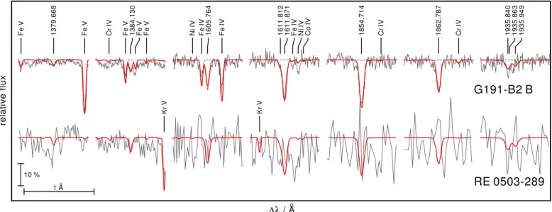
lines were identified in the UV spectrum of G191−B2B, namely λλ1854.714, 1862.787 Å (Holberg et al. 1998) and λλ1379.668, 1384.130, 1605.764, 1611.812, 1611.854 Å (Rauch et al. 2013, logarithmic mass fraction of Al= −4.95 ± 0.2).

The only additional Al lines found in the observed spectra of G191−B2B are AlIIIλλ 1935.840, 1935.863, and 1935.949 Å

(Fig.4). Al

_iv

lines in our model are entirely too weak to de-tect them in the observations. Compared to the available STIS spectrum of G191−B2B, that of RE 0503−289 has a much lower signal-to-noise ratio (S/N) that hampers detection of Al lines. AlIIIλλ 1384.130 Å is the only line that is present in the

observa-tion and is well reproduced at a solar Al abundance (−4.28±0.2). This result is based on a single line only, and thus it must be judged as uncertain. It is, however, at least an upper abundance limit. The derived abundance is, nonetheless, in good agreement with the expectation (interpolation in Fig.10). To improve the Al abundance measurement, better UV spectra for RE 0503−289 are highly desirable.

6. Zirconium

6.1. Oscillator-strength calculations for ZrIV–VIIions

Radiative decay rates (oscillator strengths and transition prob-abilities) were computed using the pseudo-relativistic Hartree-Fock (HFR) method originally introduced by Cowan (1981), and modified for taking into account core-polarization effects

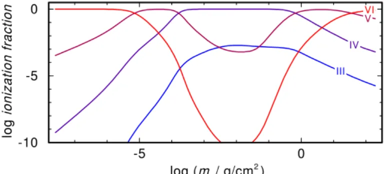
III IV V VI -10 -5 0 -5 0 log (m / g/cm2₎ l o g i o n iz a ti o n f ra c ti o n

Fig. 2.Al ionization fractions in our G191−B2B model. m is the column mass, measured from the outer boundary of our model atmospheres.

III IV V VI -10 -5 0 -5 0 log (m / g/cm2₎ l o g i o n iz a ti o n f ra c ti o n

Fig. 3.As Fig.2, for RE 0503−289.

(CPOL), giving rise to the HFR+CPOL approach (e.g., Quinet et al. 1999,2002).

For Zr

_iv

, configuration interaction was considered among the configurations 4s2_4p6_{nd (n = 4–9), 4s}2_4p6_{ns (n = 5–}

9), 4s2_4p6_{ng (n = 5–9), 4s}2_4p6_{ni (n = 7–9), 4s}2_4p5_4d5p,

4s2_4p5_{4d4f, and 4s}2_4p5_{4d5f for the even parity, and 4s}2_4p6_np

(n = 5–9), 4s2_4p6_{nf (n = 4–9), 4s}2_4p6_{nh (n= 6–9), 4s}2_4p6_nk

(n= 8–9), 4s24p54d2, 4s24p54d5s, and 4s24p54d5d for the odd parity. The core-polarization parameters were the dipole polar-izability of a Zr

_vi

ionic core as reported byFraga et al.(1976), that is, αd= 2.50 a.u., and the cut-off radius corresponding to the

HFR mean value hri of the outermost core orbital (4p), that is, rc= 1.34 a.u. Using the experimental energy levels taken from

the analysis by Reader & Acquista (1997), the average ener-gies and spin-orbit parameters of 4s24p6nd (n= 4–6), 4s24p6ns (n = 5–8), 4s2_4p6_{ng (n= 5–9), 4s}2_4p6_{np (n= 5–7), 4s}2_4p6_nf

(n = 4–6), and 4s24p66h configurations were adjusted using a well-established least-squares fitting procedure in which the mean deviations with experimental data were found to be equal to 0 cm−1_{for the even parity and 6 cm}−1_{for the odd parity.}

For Zr

_v

, the configurations explicitly included in the HFR model were 4s24p6, 4s24p5np (n = 5–7), 4s24p5nf (n = 4–7), 4s4p6_{nd (n= 4–7), 4s4p}6_{ns (n= 5–7), 4s}2_4p4_4d2_{, 4s}2_4p4_4d5s,

and 4s2_4p4_5s2 _{for the even parity, and 4s}2_4p5_{nd (n = 4–7),}

4s24p5ns (n = 5–10), 4s24p5ng (n = 5–7), 4s4p6np (n = 5– 7), 4s4p6_{nf (n = 4–7), 4s}2_4p4_{4d5p, and 4s}2_4p4_{4d4f for the}

odd parity. Core-polarization effects were estimated using αd=

0.08 a.u. and rc = 0.45 a.u. These values correspond to a

Ni-like Zr

_xiii

ionic core, with 3d as an outermost core subshell. In this ion, the semi-empirical process was performed to opti-mize the average energies, spin-orbit parameters, and electro-static interaction. Slater integrals corresponding to 4p6_{, 4p}5_np

(n = 5–6), 4p5_{4f, 4s4p}6_{4d, 4p}5_{nd (n = 4–7), 4p}5_{ns (n = 5–}

10), 4p5ng (n = 5–6), and 4s4p65p configurations using the experimental levels reported byReader & Acquista(1979) and

10 % 1 Ao

G191-B2 B

RE 0503-289

re la ti v e f lu x ∆λ / Ao F e V 1 3 7 9 .6 6 8 F e V C r IV F e V 1 3 8 4 .1 3 0 F e V F e V N i IV F e IV 1 6 0 5 .7 6 4 F e IV 1 6 1 1 .8 1 2 1 6 1 1 .8 7 1 F e IV N i IV C o IV 1 8 5 4 .7 1 4 C r IV 1 8 6 2 .7 8 7 C r IV 1 9 3 5 .8 4 0 1 9 3 5 .8 6 3 1 9 3 5 .9 4 9 K r V K r V

Fig. 4.Comparison of sections of the STIS spectra with our models for G191−B2B (top) and RE 0503−289 (bottom). The Al abundances are 1.1 × 10−5_{(0.2 times the solar value, Rauch et al. 2013) and 5.3 × 10}−5_{(solar), respectively. In the top part, the green dashed line is a spectrum}

calculated without Al. Prominent lines are marked, the identified Al

iii

lines with their wavelengths.

IV V VI VIIVIII -10 -5 0 -5 0 log (m / g/cm2₎ l o g i o n iz a ti o n f ra c ti o n

Fig. 5.Like Fig.2, for Zr.

Khan et al.(1981). The mean deviations between calculated and experimental energies were 77 cm−1 and 91 cm−1 for even and odd parities, respectively.

In the case of Zr

_vi

, the HFR method was used with the in-teracting configurations 4s24p5, 4s24p4np (n = 5–6), 4s24p4nf (n= 4–6), 4s4p5_{nd (n= 4–6), 4s4p}5_{ns (n= 5–6), 4p}6_{np (n= 5–}

6), 4p6_{nf (n = 4–6), 4s}2_4p3_4d2_{, 4s}2_4p3_{4d5s, and 4s}2_4p3_5s2 _for

the odd parity, and 4s4p6, 4s24p4nd (n= 4–6), 4s24p4ns (n= 5– 6), 4s2_4p4_{ng (n = 5–6), 4s4p}5_{np (n = 5–6), 4s4p}5_{nf (n= 4–6),}

4p6ns (n= 5–6), 4p6nd (n= 4–6), 4s24p34d5p, and 4s24p34d4f for the even parity. Core-polarization effects were estimated us-ing the same αdand rcvalues as those considered in Zr

v

. The

ra-dial integrals corresponding to 4p5_{, 4p}4_{5p, 4s4p}6_{, 4p}4_{5d, 4p}4_5s,

and 4p4_{6s were adjusted to minimize the differences between the}

calculated Hamiltonian eigenvalues and the experimental energy levels taken fromReader & Lindsay(2016). In this process, we found mean deviations equal to 111 cm−1in the odd parity and 221 cm−1_{in the even parity.}

Finally, for Zr

_vii

, the configurations included in the HFR model were 4s24p4, 4s24p3np (n = 5–6), 4s24p3nf (n = 4– 6), 4s4p4_{nd (n = 4–6), 4s4p}4_{ns (n = 5–6), 4p}5_{np (n = 5–}

6), 4p5nf (n = 4–6), 4s24p24d2, 4s24p24d5s, and 4s24p25s2 for the even parity, and 4s4p5_{, 4s}2_4p3_{nd (n = 4–6), 4s}2_4p3_ns

(n = 5–6), 4s2_4p3_{ng (n = 5–6), 4s4p}4_{np (n = 5–6), 4s4p}4_nf

(n = 4–6), 4p5ns (n = 5–6), 4p5nd (n = 4–6), 4s24p24d5p, and 4s2_4p2_{4d4f for the odd parity. The same core-polarization}

IV V VI VII VIII -10 -5 0 -5 0 log (m / g/cm2₎ l o g i o n iz a ti o n f ra c ti o n

Fig. 6.Like Fig.3, for Zr.

parameters as those used in Zr

_v

and Zr

_vi

calculations were con-sidered while the radial integrals of 4p4_{, 4p}3_{5p, 4s4p}5_{, 4p}3_4d,

and 4p35s were optimized with the experimental energy levels taken fromReader & Acquista(1976),Rahimullah et al.(1978), Khan et al. (1983). Although having established level values, the 4p3_{4f configuration was not fitted because it appeared very}

strongly mixed with experimentally unknown configurations such as 4s4p44d, and 4s24p24d2 according to our HFR calcu-lations. This semi-empirical process led to mean deviations of 695 cm−1and 479 cm−1for even and odd parities, respectively.

The parameters adopted in our computations are summa-rized in TablesA.1–A.4 while computed and available experi-mental energies are compared in TablesA.5–A.8, for Zr

_iv–vii

, respectively. Tables A.9–A.12 give the HFR weighted oscilla-tor strengths (log g f ) and transition probabilities (gA, in s−1) to-gether with the numerical values (in cm−1_{) of the lower and}

up-per energy levels and the corresponding wavelengths (in Å). In the last column of each table, we also give the cancellation fac-tor, CF, as defined byCowan(1981). We note that very low val-ues of this factor (typically <0.05) indicate strong cancellation effects in the calculation of line strengths. In these cases, the corresponding g f and gA values could be very inaccurate and therefore need to be considered with some care. However, very few of the transitions appearing in Tables A.9–A.12 are affected.

Zr V

Zr IV

Zr VI

re la ti v e f lu x ∆λ / Ao 10 % 1 Ao F e V 1 0 0 1 .7 6 5 u n id . C II I 1 0 0 2 .4 8 4 G a V F e V Z n V G e V 1 0 6 8 .5 5 1 G a V 1 0 6 8 .8 3 6 Z n V Z n V Z n V 1 1 1 9 .1 5 8 N i V I M o V Z n V 1 2 0 0 .7 6 0 1 2 0 0 .8 0 2 M o V 1 2 0 0 .9 4 3 M o IV 1 2 4 5 .9 5 1 N i V N i V N i V 1 2 6 0 .9 0 9 Z n V N i V Z n V 1 2 6 5 .3 8 1 G a V N i V N i V G a IV 1 3 0 3 .9 3 3 N i V Z n V 1 3 0 6 .7 6 2 N i V 1 3 2 3 .8 2 6 N i V N i V 1 3 3 2 .0 6 5 1 3 5 5 .2 1 6 N i V 1 3 5 5 .9 7 5 M o V Z n V Z n V N i V F e V F e V 1 3 7 6 .5 4 4 1 6 3 3 .0 2 7 1 7 2 5 .0 2 4 Z n V 1 0 5 3 .5 4 8 Z n V G e V 1 0 6 4 .8 1 8 1 0 9 9 .5 9 1 M o V Z n V G a V B a V 1 1 1 8 .6 8 9 Z n V Z n V 1 5 9 8 .9 4 8 N i V I Z n V Z n V 1 1 5 1 .5 7 1 Z n V 1 1 5 1 .8 5 9 N i V 1 5 1 4 .5 6 8 1 5 2 1 .6 9 9 C II I 1 5 9 1 .7 9 9 F e IV 1 6 8 2 .2 4 1 K r V I 1 7 4 9 .3 5 0

Fig. 7.Identified Zr

_iv

(bottom of right panel), Zr

_v

(left panel), and Zr

_vi

(right panel) lines in the FUSE (λ < 1188 Å) and HST/STIS observations of RE 0503−289. The model (thick, red line) was calculated with an abundance of log Zr = −3.5. The dashed green spectrum was calculated without Zr. Prominent lines are marked, the Zr lines with their wavelengths from Tables A.9–A.11.

These tables are provided via the registered GAVO Tübingen Os-cillator Strengths Service (TOSS7).

6.2. Zr line identification and abundance analysis

In the FUSE and HST/STIS observations of RE 0503−289, we identified Zr

_iv–vi

lines (Table4). The observation is well

7 _{http://dc.g-vo.org/TOSS}

reproduced by our model calculated with a mass fraction of log Zr= −3.5 ± 0.2 (Fig.7). The Zr

_iv/v/vi

ionization equilibria are matched by our model.

In our synthetic spectra for G191−B2B, ZrIVλ 1598.948 Å

is the strongest line. A comparison with the STIS spectrum shows that a Zr mass fraction of 2.6 × 10−6 _{(approximately}

100 times solar,Grevesse et al. 2015) is the upper detection limit (Fig.8).

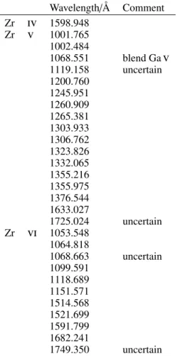
Table 4. Identified Zr lines in the UV spectrum of RE 0503−289. Wavelength/Å Comment Zr

_iv

1598.948 Zr

_v

1001.765 1002.484 1068.551 blend Ga

_v

1119.158 uncertain 1200.760 1245.951 1260.909 1265.381 1303.933 1306.762 1323.826 1332.065 1355.216 1355.975 1376.544 1633.027 1725.024 uncertain Zr

_vi

1053.548 1064.818 1068.663 uncertain 1099.591 1118.689 1151.571 1514.568 1521.699 1591.799 1682.241 1749.350 uncertain

Notes. The wavelengths correspond to those in Tables A.9–A.11.

7. Xenon

7.1. Oscillator-strength calculations for XeIV,V, andVIIions New calculations of oscillator strengths and radiative transi-tion probabilities in xenon ions were also performed using the HFR+CPOL method (Cowan 1981;Quinet et al. 1999,2002).

For Xe

_iv

, the multiconfiguration expansion included 5s2_5p3_,

5s2_5p2_{6p, 5s}2_5p2_{nf (n= 4–6), 5s}2_{5p5d6s, 5s}2_{5p5d6d, 5s}2_5p6s2_,

5s2_5p5d2_{, 5s}2_5p4f2_{, 5s5p}3_{6s, 5s5p}3_{nd (n= 5–6), 5s5p}2_{4f5d, and}

5p5_{for the odd parity, and 5s5p}4_{, 5s}2_5p2_{nd (n= 5–6), 5s}2_5p2_6s,

5s25p2ng (n= 5–6), 5s25p5d6p, 5s25p5dnf (n= 4–6), 5s5p36p, 5s5p3_{nf (n= 4–6), and 5s5p}2_5d2 _{for the even parity. The}

core-polarization effects were estimated with αd = 0.88 a.u. and rc

= 0.86 a.u. which correspond to a Pd-like Xe

ix

ionic core. The former value was taken from Fraga et al.(1976) while the lat-ter one corresponds to the HFR mean value hri of the oulat-termost core orbital (4d). The experimental energy levels published by Saloman(2004) were then used to optimize the radial parame-ters belonging to the 5p3_{, 5p}2_{6p, 5p}2_{4f, 5s5p}4_{, 5p}2_{5d, and 5p}2_6s

configurations allowing us to reach average deviations between calculated and observed energies of 137 cm−1_{and 251 cm}−1_{, for}

odd and even parities, respectively.

In the case of Xe

_v

, the following sets of configurations were considered in the HFR model: 5s25p2, 5s25p6p, 5s25pnf (n= 4– 6), 5s2_{5d6s, 5s}2_{5d6d, 5s}2_6s2_{, 5s}2_5d2_{, 5s}2_4f2_{, 5s}2_5f2_{, 5s5p}2_6s,

5s5p2_{nd (n = 5–6), 5s5p6s6p, 5s5p6pnd (n = 5–6), 5s5p4fnd}

(n = 5–6), 5p4, 5p36p, and 5p3nf (n = 4–6) for the even par-ity, and 5s5p3_{, 5s}2_{5pnd (n = 5–6), 5s}2_{5pns (n= 6–7), 5s}2_5png

Zr IV

re la ti v e f lu x 10 % F e IV F e IV F e V F e V 1 5 9 8 .9 4 8 -0.8 -0.6 -0.4 -0.2 0.0 0.2 ∆λ / Ao

Fig. 8. Section of the STIS spectrum of G191−B2B around Zr

_iv

λ 1598.948 Å compared with three synthetic spectra (thin, blue: no Zr, thick, red: Zr mass fraction= 2.6 × 10−6_{, dashed green: Zr=}

2.6 × 10−5_).

(n = 5–6), 5s2_{5d6p, 5s}2_{5dnf (n = 4–6), 5s5p}2_{6p, 5s5p}2_nf

(n = 4–6), 5s5p6snd (n = 5–6), 5s5p5d6d, 5s5p6s2, 5s5p5d2, 5p3_{6s, and 5p}3_{nd (n= 5–6) for the odd parity. The same}

core-polarization parameters as those used for Xe

_iv

were used and the experimental energy levels reported bySaloman(2004) and Raineri et al.(2009) were incorporated into the semi-empirical fit to adjust the radial integrals corresponding to the 5p2, 5p6p, 5p4f, 5s5p3_{, 5p5d, 5p6d, 5p6s, and 5p7s configurations. In this}

process, we found mean deviations equal to 144 cm−1in the even parity and 110 cm−1_{in the odd parity.}

For Xe

_vi

, we used the same atomic data as those con-sidered in one of our previous papers (Rauch et al. 2015a). More precisely, the radiative rates were taken from the work of Gallardo et al. (2015) who performed HFR+CPOL calcula-tions including 35 odd-parity and 34 even-parity configuracalcula-tions, that is, 5s2_{np (n = 5–8), 5s}2_{nf (n = 4–8), 5s}2_{nh (n = 6–8),} 5s28k, 5p2np (n = 6–8), 5p2nf (n = 4–8), 5p2nh (n = 6–8), 5p2_{8k, 5s5p6s, 5s5pnd (n= 5–6), 5s5png (n = 5–6), 5p}3_{, 5s5dnf} (n= 4–5), 5s6snf (n = 4–5), and 5s5p2, 5s2ns (n= 6–8), 5s2nd (n = 5–8), 5s2_{ng (n = 5–8), 5s}2_{ni (n= 7–8), 5p}2_{nd (n = 5–} 8), 5p2ns (n= 6–8), 5p2ng (n = 5–8), 5p2ni (n= 7–8), 5s5pnf (n = 4–6), 5s4f2_{, 5s5f}2_{, 5s5p6p, 4d}9_5p4_{, respectively. In this}

latter study, the core-polarization effects were considered with two different ionic cores, that is, a Cd-like Xe

_vii

core with αd = 5.80 a.u. for the 5s2nl–5s2n0l0 transitions, and a Pd-like

Xe

_ix

core with αd = 0.99 a.u. for all the other transitions. In

their semi-empirical least-squares fitting process,Gallardo et al. (2015) achieved standard deviations with experimental energy levels of 149 cm−1 _{in the odd parity and 154 cm}−1 _{in the even}

parity.

Finally, for Xe

_vii

, we used the same model as the one con-sidered byBiémont et al.(2007) extending the set of oscillator strengths to weaker transitions (up to log g f > −8). As a re-minder, these authors explicitly retained the following config-urations in their configuration interaction expansions: 5s2_{, 5p}2_,

5d2, 4f2, 4fnp (n= 5–6), 4f6f, 4f6h, 5s6s, 5snd (n = 5–6), 5sng (n = 5–6), 5pnf (n = 5–6), 5p6p, 5p6h, 5d6s, 5d6d, and 5dng (n= 5–6) for the even parity, and 5snp (n = 5–6), 5snf (n = 4–6), 5s6h, 4f6s, 4fnd (n= 5–6), 4fng (n = 5–6), 5p6s, 5pnd (n = 5– 6), 5png (n = 5–6), 5d6p, and 5dnf (n = 5–6), 5d6h for the odd parity. The same ionic core parameters as those used for Xe IV and Xe V ions were considered and all the experimental en-ergy levels published bySaloman (2004) were included in the semi-empirical optimization of the radial parameters belonging

Xe VI

Xe VII

re la ti v e f lu x ∆λ / Ao 10 % 1 Ao H Iis 9 1 5 .1 6 3 H Iis 1 0 8 0 .0 8 0 Z n V G e V 1 1 8 1 .4 6 0 1 1 8 1 .5 4 0 1 1 8 1 .7 5 0 O IV 9 9 5 .5 1 6 M o V I 9 2 8 .3 6 6 M o V 1 0 9 1 .6 3 0 Z n V M o V 1 1 8 4 .3 9 0 M o V N i V I Z n V N i V I 1 0 7 7 .1 2 0 9 2 9 .1 3 1 G e V I G a V M o V 1 1 0 1 .9 4 0 B a V 1 2 2 8 .4 5 0 Z n IV M o V I N i V N i V 1 2 4 3 .5 6 5 N i V Z n V G e V I 9 6 7 .5 5 0 O II I 1 1 1 0 .4 5 0 Z n V N i V 1 2 8 0 .2 7 0 Z n IV G a V I 9 7 0 .1 7 7 G a V Z n V Z n V 1 1 3 6 .4 1 0 Z n V N i V 1 2 9 8 .9 1 0 G e V 1 0 1 7 .2 7 0 Z n V 1 1 7 9 .5 4 0 Z n V 1 4 3 9 .2 5 0

Fig. 9.Identified Xe

vi

(top three rows) and Xe

vii

(bottom row) lines in the FUSE (λ < 1188 Å) and HST/STIS observations of RE 0503−289. The

model (thick, red line) was calculated with an abundance of log Xe = −3.9. The dashed, green spectrum was calculated without Xe. Prominent lines are marked (“is” denotes interstellar origin), and the Xe lines are labelled with their wavelengths given byGallardo et al.(2015) and in Table B.7. HHe C ON Al PSi S Ti Cr Fe Ni Zn GeMn Co GaAs Kr Zr Mo Sn Xe Ba lo g m a s s f ra c ti o n G 191-B2B RE 0503-289 -5 0 [X ] -4 -2 0 2 4 10 20 30 40 50 atomic number

Fig. 10. Solar abundances (Asplund et al. 2009; Scott et al. 2015b,a;

Grevesse et al. 2015, thick line; the dashed lines connect the ele-ments with even and with odd atomic number) compared with the determined photospheric abundances of G191−B2B (blue circles,

Rauch et al. 2013) and RE 0503−289 (red squares,Dreizler & Werner 1996; Rauch et al. 2012, 2014a,b, 2015a,b, 2016a,b, and this work). The uncertainties of the WD abundances are, in general, approximately 0.2 dex. The arrows indicate upper limits. Top panel: abundances given as logarithmic mass fractions. Bottom panel: abundance ratios to respec-tive solar values, [X] denotes log (fraction/solar fraction) of species X. The dashed green line indicates solar abundances.

to the 5s2_{, 5s6s, 5s5d, 5s6d, 5p}2_{, 4f5p, 5s5p, 5s6p, 5s4f, 5s5f,}

5p6s, and 5p5d configurations giving rise to standard deviations of 377 cm−1 _{and 250 cm}−1 _{for even- and odd-parity levels,}

re-spectively.

The radial parameters used in our computations are summa-rized in Tables B.1, B.2 for the Xe

_iv–v

ions, respectively. The calculated energy levels are compared with available experimen-tal values in Tables B.3, B.4 while the HFR weighted oscillator strengths (log g f ) and transition probabilities (gA in s−1) are re-ported in Tables B.5–B.7 for the Xe

_iv–v

and

_vii

ions, respec-tively. In the latter tables, we also give the numerical values (in cm−1_{) of lower and upper energy levels of each transition}

to-gether with the corresponding wavelength (in Å) and the CF, as introduced in Sect.6.1. These tables are provided via TOSS.

7.2. Xe line identification and abundance analysis

In the FUSE and HST/STIS observations of RE 0503−289, we identified Xe

_vi-vii

lines (Table5). The observation is well re-produced by our model, calculated with a mass fraction of log Xe= −3.9 ± 0.2 (Fig.9). This is a factor of two higher than that previously determined by Werner et al. (2012b, log Xe = −4.2 ± 0.6) but agrees within their given error limits. The

Xe

_vi/vii

ionization equilibrium is matched by our model.

8. Results and conclusions

To search for Al lines in the observed UV spectrum of RE 0503−289, we created an extended Al model atom for our NLTE model-atmosphere calculations. We could only identify AlIIIλλ 1384.130 Å (Sect.5), that was well suited to measure the

N Al P Ga As He C O Si S Ni Zn Ge Kr Zr Mo Sn Xe Ba 0 5 10 20 30 40 50 60 70 80 atomic number [ X /O ]

Fig. 11. Determined photospheric abundances of RE 0503−289 (cf. Fig.10) compared with predictions for surface abundances of

Karakas & Lugaro(2016, for an asymptotic giant branch (AGB) star with Minitial = 1.5 M, Mfinal = 0.585 M, metallicity Z = 0.014). [X/O]

denotes the normalized log [(fraction of X/solar fraction of X)/(fraction of O/solar fraction of O)] mass ratio. The dashed green line indicates the solar ratio.

Table 5. Identified Xe lines in the UV spectrum of RE 0503−289.

Wavelength/Å Comment Xe

_vi

915.163 weak 928.366a 929.131b 967.550a 970.177 weak 1017.270b 1080.080a 1091.630a 1101.940a 1110.450 weak 1136.410a 1179.540a 1181.390a 1181.540 blend with Xe

_vi

λ 1181.390 Å 1184.390a uncertain 1228.450 1280.270 1298.910b 1439.250 Xe

_vii

995.516a 1077.120a 1243.565

Notes. The wavelengths correspond to those given inGallardo et al.

(2015) and in Table B.7 for Xe

_vi

and Xe

_vii

, respectively.(a)

Identi-fied byWerner et al.(2012b);(b)_{identified byRauch et al.(2015a).}

fraction). This needs to be verified once better observations are available.

We identified Zr

_iv–vi

lines in the observed high-resolution UV spectra RE 0503−289 (Table4). These were well modeled using our newly calculated Zr

_iv–vii

oscillator strengths. We de-termined a photospheric abundance of log Zr = −3.52 ± 0.2 (mass fraction, 1.5−4.8 × 10−4, 5775–14 480 times the so-lar abundance). This highly supersoso-lar Zr abundance corre-sponds to the high abundances of other trans-iron elements in RE 0503−289 (Fig.10). The Zr

_iv/v/vi

ionization equilibria are well matched by our model (Teff= 70 000 K, log g = 7.5).

In addition to the previously discovered Xe

_vi–vii

lines in the UV spectrum of RE 0503−289, we identified five new Xe

_vi

lines. All identified Xe lines are well matched by our model with an abundance of log Xe = −3.88 ± 0.2 (mass frac-tion, 0.8−2.1 × 10−4, 4985–12 520 times the solar abundance). This highly supersolar Xe abundance is in line with abundances of other trans-iron elements in RE 0503−289 (Fig.10).

The amount of trans-iron elements in the photosphere of RE 0503−289 strongly exceeds the yields of nucleosynthesis on the asymptotic giant branch (Fig11). It is likely that radiative levitation is working efficiently in RE 0503−289 (Rauch et al. 2016a), increasing abundances by up to 4 dex compared with so-lar values.

The identification of lines of Zr and Xe and their precise abundance determinations only became possible after reliable transition probabilities for Zr

_iv–vii

, Xe

_iv–v

, and Xe

_vii

were computed. Calculations for other, highly-ionized trans-iron ele-ments are necessary to search for their lines and to measure their abundances.

The search for Zr and Xe lines in the UV spectrum of G191−B2B was entirely negative. We established an upper Zr abundance limit of approximately 100 times solar and con-firmed the previously found upper limit for Xe of approximately 10 times solar (Rauch et al. 2016a).

Acknowledgements. T.R. and D.H. are supported by the German Aerospace Center (DLR, grants 05 OR 1507 and 50 OR 1501, respectively). The GAVO project had been supported by the Federal Ministry of Education and Research (BMBF) at Tübingen (05 AC 6 VTB, 05 AC 11 VTB) and is funded at Heidelberg (05 AC 11 VH3). Financial support from the Belgian FRS-FNRS is also acknowl-edged. P.Q. is research director of this organization. Some of the data presented in this paper were obtained from the Mikulski Archive for Space Telescopes (MAST). STScI is operated by the Association of Universities for Research in Astronomy, Inc., under NASA contract NAS5-26555. Support for MAST for non-HST data is provided by the NASA Office of Space Science via grant NNX09AF08G and by other grants and contracts. This research has made use of NASA’s Astrophysics Data System and the SIMBAD database, operated at CDS, Strasbourg, France. The TOSS service (http://dc.g-vo.org/TOSS) that pro-vides weighted oscillator strengths and transition probabilities was constructed as part of the activities of the German Astrophysical Virtual Observatory.

References

Asplund, M., Grevesse, N., Sauval, A. J., & Scott, P. 2009,ARA&A, 47, 481

Bohlin, R. C. 2007, in The Future of Photometric, Spectrophotometric and Polarimetric Standardization, ed. C. Sterken, ASP Conf. Ser., 364, 315 Cowan, R. D. 1981, in The theory of atomic structure and spectra (Berkeley, CA:

University of California Press)

Cowley, C. R. 1970, in The theory of stellar spectra (New York: Gordon & Breach)

Cowley, C. R. 1971,The Observatory, 91, 139

Dreizler, S., & Werner, K. 1996,A&A, 314, 217

Fraga, S., Karwowski, J., & Saxena, K. M. S. 1976, in Handbook of Atomic Data (Amsterdam: Elsevier)

Gallardo, M., Raineri, M., Reyna Almandos, J., Pagan, C. J. B., & Abrahão, R. A. 2015,ApJS, 216, 11

Grevesse, N., Scott, P., Asplund, M., & Sauval, A. J. 2015,A&A, 573, A27

Holberg, J. B., Barstow, M. A., & Sion, E. M. 1998,ApJS, 119, 207

Hubeny, I., Hummer, D. G., & Lanz, T. 1994,A&A, 282, 151

Hummer, D. G., & Mihalas, D. 1988,ApJ, 331, 794

Karakas, A. I., & Lugaro, M. 2016,ApJ, 825, 26

Khan, Z. A., Rahimullah, K., & Chaghtai, M. S. Z. 1981,Phys. Scr., 23, 843

Khan, Z. A., Chaghtai, M. S. Z., & Rahimullah, K. 1983,J. Phys. B: At. Mol. Phys., 16, 1685

Lemoine, M., Vidal-Madjar, A., Hébrard, G., et al. 2002,ApJS, 140, 67

McCook, G. P., & Sion, E. M. 1999a,ApJS, 121, 1

McCook, G. P., & Sion, E. M. 1999b,VizieR Online Data Catalog: III/210 Müller-Ringat, E. 2013, Dissertation, University of Tübingen, Germany,http:

//www.ivoa.net/documents/SimDM/index.html

Quinet, P., Palmeri, P., Biémont, É., et al. 1999,MNRAS, 307, 934

Quinet, P., Palmeri, P., Biémont, É., et al. 2002,J. Alloys Comp., 344, 255

Rahimullah, K., Chaghtai, M. S. Z., & Khatoon, S. 1978,Physica Scripta, 18, 96

Raineri, M., Gallardo, M., Padilla, S., & Reyna Almandos, J. 2009,J. Phys. B, 42, 205004

Rauch, T., & Deetjen, J. L. 2003, in Stellar Atmosphere Modeling, eds. I. Hubeny, D. Mihalas, & K. Werner, ASP Conf. Ser., 288, 103

Rauch, T., Werner, K., Biémont, É., Quinet, P., & Kruk, J. W. 2012,A&A, 546, A55

Rauch, T., Werner, K., Bohlin, R., & Kruk, J. W. 2013,A&A, 560, A106

Rauch, T., Werner, K., Quinet, P., & Kruk, J. W. 2014a,A&A, 564, A41

Rauch, T., Werner, K., Quinet, P., & Kruk, J. W. 2014b,A&A, 566, A10

Rauch, T., Hoyer, D., Quinet, P., Gallardo, M., & Raineri, M. 2015a,A&A, 577, A88

Rauch, T., Werner, K., Quinet, P., & Kruk, J. W. 2015b,A&A, 577, A6

Rauch, T., Quinet, P., Hoyer, D., et al. 2016a,A&A, 587, A39

Rauch, T., Quinet, P., Hoyer, D., et al. 2016b,A&A, 590, A128

Reader, J., & Acquista, N. 1976,J. Opt. Soc. Am., 66, 896

Reader, J., & Acquista, N. 1979,J. Opt. Soc. Am., 69, 239

Reader, J., & Acquista, N. 1997,J. Opt. Soc. Am. B, 14, 1328

Reader, J., & Lindsay, M. D. 2016,Phys. Scr., 91, 025401

Saloman, E. B. 2004,J. Phys. Chem. Ref. Data, 33, 765

Scott, P., Asplund, M., Grevesse, N., Bergemann, M., & Sauval, A. J. 2015a,

A&A, 573, A26

Scott, P., Grevesse, N., Asplund, M., et al. 2015b,A&A, 573, A25

Werner, K., Deetjen, J. L., Dreizler, S., et al. 2003, in Stellar Atmosphere Modeling, eds. I. Hubeny, D. Mihalas, & K. Werner, ASP Conf. Ser., 288, 31

Werner, K., Dreizler, S., & Rauch, T. 2012a, Astrophysics Source Code Library

[record ascl:1212.015]

Appendix A: Additional tables for zirconium

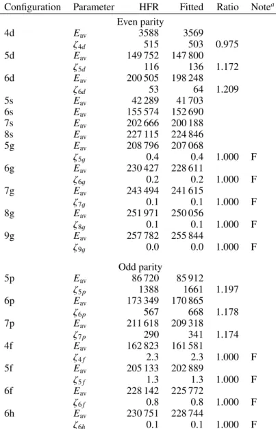
Table A.1. Radial parameters (in cm−1_{) adopted for the calculations in Zr}

iv

.

Configuration Parameter HFR Fitted Ratio Notea

Even parity 4d Eav 3588 3569 ζ4d 515 503 0.975 5d Eav 149 752 147 800 ζ5d 116 136 1.172 6d Eav 200 505 198 248 ζ6d 53 64 1.209 5s Eav 42 289 41 703 6s Eav 155 574 152 690 7s Eav 202 666 200 188 8s Eav 227 115 224 846 5g Eav 208 796 207 068 ζ5g 0.4 0.4 1.000 F 6g Eav 230 427 228 611 ζ6g 0.2 0.2 1.000 F 7g Eav 243 494 241 615 ζ7g 0.1 0.1 1.000 F 8g Eav 251 971 250 056 ζ8g 0.1 0.1 1.000 F 9g Eav 257 782 255 844 ζ9g 0.0 0.0 1.000 F Odd parity 5p Eav 86 720 85 912 ζ5p 1388 1661 1.197 6p Eav 173 349 170 865 ζ6p 567 668 1.178 7p Eav 211 618 209 318 ζ7p 290 341 1.174 4f Eav 162 823 161 581 ζ4 f 2.3 2.3 1.000 F 5f Eav 205 133 202 889 ζ5 f 1.3 1.3 1.000 F 6f Eav 228 142 225 772 ζ6 f 0.8 0.8 1.000 F 6h Eav 230 751 228 744 ζ6h 0.1 0.1 1.000 F

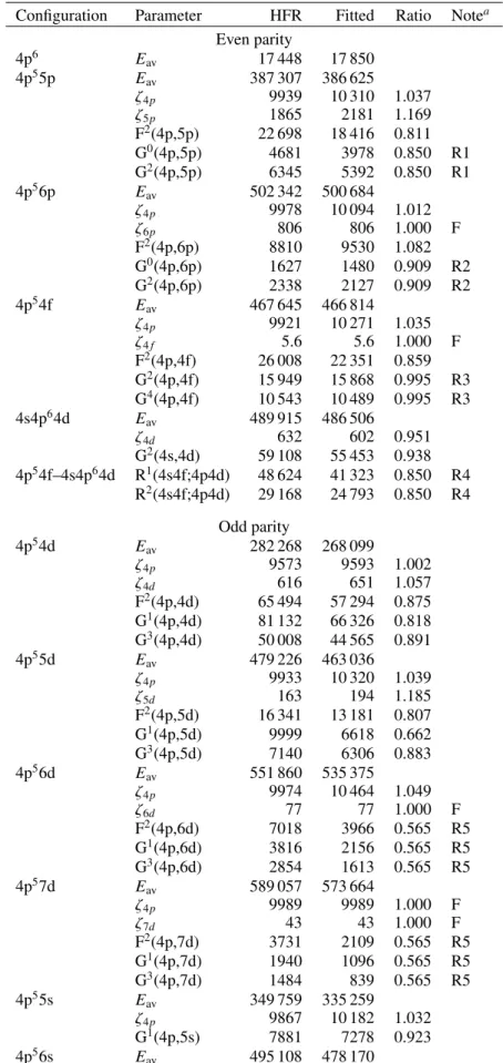
Table A.2. Radial parameters (in cm−1_{) adopted for the calculations in Zr}

v

.

Configuration Parameter HFR Fitted Ratio Notea Even parity 4p6 Eav 17 448 17 850 4p5_{5p E} av 387 307 386 625 ζ4p 9939 10 310 1.037 ζ5p 1865 2181 1.169 F2_{(4p,5p) 22 698 18 416 0.811} G0(4p,5p) 4681 3978 0.850 R1 G2_{(4p,5p) 6345 5392 0.850 R1} 4p5_{6p E} av 502 342 500 684 ζ4p 9978 10 094 1.012 ζ6p 806 806 1.000 F F2(4p,6p) 8810 9530 1.082 G0_{(4p,6p) 1627 1480 0.909 R2} G2_{(4p,6p) 2338 2127 0.909 R2} 4p54f Eav 467 645 466 814 ζ4p 9921 10 271 1.035 ζ4 f 5.6 5.6 1.000 F F2_{(4p,4f) 26 008 22 351 0.859} G2_{(4p,4f) 15 949 15 868 0.995 R3} G4(4p,4f) 10 543 10 489 0.995 R3 4s4p6_{4d E} av 489 915 486 506 ζ4d 632 602 0.951 G2_{(4s,4d) 59 108 55 453 0.938} 4p54f–4s4p64d R1(4s4f;4p4d) 48 624 41 323 0.850 R4 R2_{(4s4f;4p4d) 29 168 24 793 0.850 R4} Odd parity 4p54d Eav 282 268 268 099 ζ4p 9573 9593 1.002 ζ4d 616 651 1.057 F2(4p,4d) 65 494 57 294 0.875 G1_{(4p,4d) 81 132 66 326 0.818} G3(4p,4d) 50 008 44 565 0.891 4p5_{5d E} av 479 226 463 036 ζ4p 9933 10 320 1.039 ζ5d 163 194 1.185 F2_{(4p,5d) 16 341 13 181 0.807} G1(4p,5d) 9999 6618 0.662 G3_{(4p,5d) 7140 6306 0.883} 4p56d Eav 551 860 535 375 ζ4p 9974 10 464 1.049 ζ6d 77 77 1.000 F F2(4p,6d) 7018 3966 0.565 R5 G1_{(4p,6d) 3816 2156 0.565 R5} G3_{(4p,6d) 2854 1613 0.565 R5} 4p5_{7d E} av 589 057 573 664 ζ4p 9989 9989 1.000 F ζ7d 43 43 1.000 F F2_{(4p,7d) 3731 2109 0.565 R5} G1(4p,7d) 1940 1096 0.565 R5 G3_{(4p,7d) 1484 839 0.565 R5} 4p5_{5s E} av 349 759 335 259 ζ4p 9867 10 182 1.032 G1_{(4p,5s) 7881 7278 0.923} 4p56s Eav 495 108 478 170

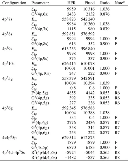
Table A.2. continued.

Configuration Parameter HFR Fitted Ratio Notea

ζ4p 9959 10 316 1.036 G1_{(4p,6s) 2433 2132 0.876} 4p57s Eav 558 823 542 240 ζ4p 9984 10 360 1.038 G1(4p,7s) 1115 980 0.879 4p5_{8s E} av 592 851 576 592 ζ4p 9994 9994 1.000 F G1(4p,8s) 613 552 0.900 F 4p5_{9s E} av 613 233 596 840 ζ4p 9998 9998 1.000 F G1_{(4p,9s) 375 337 0.900 F} 4p510s Eav 626 415 610 078 ζ4p 10 001 10 001 1.000 F G1_{(4p,10s) 247 222 0.900 F} 4p55g Eav 558 379 542 891 ζ4p 10 004 10 394 1.039 ζ5g 0.8 0.8 1.000 F F2_{(4p,5g) 4855 4142 0.853 R6} G3_{(4p,5g) 392 335 0.853 R6} G5_{(4p,5g) 277 236 0.853 R6} 4p5_{6g E} av 592 345 576 588 ζ4p 10 004 10 388 1.038 ζ6g 0.4 0.4 1.000 F F2(4p,6g) 2776 2436 0.877 R7 G3_{(4p,6g) 358 314 0.877 R7} G5(4p,6g) 253 222 0.877 R7 4s4p6_{5p E} av 629 514 612 875 ζ5p 1879 1879 1.000 F G1(4s,5p) 6870 6183 0.900 F 4p5_4d–4p5_{5s R}2_{(4p4d;4p5s) –8924 –5044 0.565 R8} R1(4p4d;4p5s) –1482 –837 0.565 R8

Table A.3. Radial parameters (in cm−1_{) adopted for the calculations in Zr}

vi

.

Configuration Parameter HFR Fitted Ratio Notea Odd parity 4p5 Eav 22 997 23 322 ζ4p 10 007 10 580 1.057 4p4_{5p E} av 461 912 446 765 F2(4p,4p) 84 088 79 559 0.946 α 0 –651 ζ4p 10 577 10 907 1.031 ζ5p 2382 2701 1.134 F2_{(4p,5p) 26 052 21 472 0.824} G0(4p,5p) 5535 4696 0.848 G2_{(4p,5p) 7459 6664 0.893} Even parity 4s4p6 Eav 251 206 224 383 4p4_{4d E} av 289 403 291 464 F2_{(4p,4p) 82 744 78 447 0.948} α 0 –450 ζ4p 10 187 10 521 1.033 ζ4d 721 854 1.184 F2_{(4p,4d) 69 677 62 179 0.892} G1_{(4p,4d) 86 802 72 077 0.831} G3(4p,4d) 53 829 45 721 0.849 4p4_{5d E} av 536 543 535 860 F2(4p,4p) 84 140 77 928 0.926 α 0 –450 F ζ4p 10 569 10 891 1.030 ζ5d 217 259 1.191 F2_{(4p,5d) 19 555 16 945 0.867} G1(4p,5d) 10 870 8250 0.759 R1 G3_{(4p,5d) 8037 6100 0.759 R1} 4p4_{5s E} av 386 802 387 950 F2(4p,4p) 83 739 79 833 0.953 α 0 –665 ζ4p 10 498 10 846 1.033 G1(4p,5s) 8725 7618 0.873 4p4_{6s E} av 564 837 564 005 F2(4p,4p) 84 213 81 311 0.965 α 0 –332 ζ4p 10 600 11 164 1.053 G1(4p,6s) 2787 2372 0.851 4s4p6_–4p4_{4d R}1_{(4p4p;4s4d) 96 078 72 916 0.759 R2} 4s4p6–4p45d R1(4p4p;4s5d) 32 299 24 513 0.759 R2

Table A.4. Radial parameters (in cm−1_{) adopted for the calculations in Zr}

vii

.

Configuration Parameter HFR Fitted Ratio Notea Even parity 4p4 _E av 23 653 33 968 F2(4p,4p) 84 430 65 839 0.780 α 0 646 ζ4p 10 658 11 259 1.056 4p3_{5p E} av 516 191 514 481 F2_{(4p,4p) 86 163 82 914 0.962} α 0 –537 ζ4p 11 232 11 776 1.048 ζ5p 2920 2920 1.000 F F2_{(4p,5p) 29 125 29 164 1.001} G0_{(4p,5p) 6338 6086 0.960} G2(4p,5p) 8477 5272 0.622 Odd parity 4s4p5 _E av 246 126 238 581 ζ4p 10 648 11 005 1.034 G1_{(4s,4p) 112 472 98 647 0.877} 4p34d Eav 320 698 319 713 F2(4p,4p) 84 870 81 614 0.962 α 0 –508 ζ4p 10 822 11 010 1.017 ζ4d 824 795 0.964 F2(4p,4d) 73 259 69 858 0.954 G1_{(4p,4d) 91 609 77 513 0.846} G3_{(4p,4d) 57 095 48 489 0.849} 4p35s Eav 448 971 447 229 F2_{(4p,4p) 85 823 80 727 0.941} α 0 –667 ζ4p 11 148 11 790 1.058 G1_{(4p,5s) 9475 8104 0.855} 4s4p5–4p34d R1(4p4p;4s4d) 100 074 78 158 0.781

Table A.5. Comparison between available experimental and calculated energy levels in Zr

_iv

.

Eexpa Ecalcb ∆E J Leading components (in %) in LS couplingc

Even parity 0.00 0000 0 1.5 99 4d2_D 1250.70 1251 0 2.5 99 4d2_D 38 258.35 38 258 0 0.5 99 5s2S 146 652.40 146 652 0 1.5 100 5d2_D 147 002.46 147 002 0 2.5 100 5d2_D 152 513.00 152 513 0 0.5 100 6s2S 197 765.10 197 765 0 1.5 100 6d2_D 197 930.43 197 930 0 2.5 100 6d2_D 200 123.69 200 124 0 0.5 100 7s2S 206 864.42 206 863 0 3.5 100 5g2_G 206 864.68 206 866 –1 4.5 100 5g2_G 224 813.48 224 813 0 0.5 100 8s2S 228 479.86 228 479 0 3.5 100 6g2_G 228 480.08 228 480 0 4.5 100 6g2G 241 526.36 241 526 0 3.5 100 7g2_G 241 526.52 241 527 0 4.5 100 7g2_G 249 995.33 249 995 0 3.5 100 8g2G 249 995.44 249 996 0 4.5 100 8g2_G 255 800.20 255 801 –1 3.5 100 9g2_G 255 801.50 255 801 1 4.5 100 9g2G Odd parity 81 976.50 81 976 0 0.5 99 5p2_P 84 461.35 84 461 0 1.5 99 5p2P 159 066.75 159 041 26 2.5 98 4f2_F 159 086.91 159 112 –25 3.5 98 4f2F 169 809.71 169 810 0 0.5 100 6p2P 170 815.11 170 815 0 1.5 100 6p2_P 201 114.14 201 105 9 2.5 97 5f2F 201 162.65 201 171 –9 3.5 97 5f2_F 208 783.36 208 783 0 0.5 100 7p2_P 209 297.66 209 298 0 1.5 100 7p2P 224 419.90 224 425 –5 2.5 96 6f2_F 224 488.11 224 483 5 3.5 97 6f2_F 228 743.87 228 744 0 4.5 100 6h2H 228 743.87 228 744 0 5.5 100 6h2_H Notes. Energies are given in cm−1_.(a)_{FromReader & Acquista(1997).}(b)_{This work.}

Table A.6. Comparison between available experimental and calculated energy levels in Zr

_v

.

Eexpa Ecalcb ∆E J Leading components (in %) in LS couplingc

Even parity 0.00 0 0 0 97 4p6 1_S 371 895.16 372 099 –204 1 84 4p5_5p3_{S+ 13 4p}5_5p3_P 376 897.68 376 807 91 2 57 4p5_5p3_{D+ 36 4p}5_5p1_{D+ 7 4p}5_5p3_P 378 753.36 378 653 100 3 99 4p5_5p3_D 380 855.53 380 904 –48 1 46 4p5_5p1_{P+ 30 4p}5_5p3_{D+ 20 4p}5_5p3_P 382 985.08 382 952 33 2 67 4p5_5p3_{P+ 30 4p}5_5p1_D 388 852.95 388 865 –12 0 77 4p5_5p3_{P+ 22 4p}5_5p1_S 391 998.41 392 073 –75 1 64 4p5_5p3_{D+ 33 4p}5_5p1_P 395 994.98 395 944 51 2 40 4p5_5p3_{D+ 33 4p}5_5p1_{D+ 25 4p}5_5p3_P 396 300.35 396 396 –96 1 64 4p5_5p3_{P+ 19 4p}5_5p1_{P+ 11 4p}5_5p3_S 402 688.40 402 529 160 0 76 4p5_5p1_{S+ 22 4p}5_5p3_P 434 714.60 434 703 12 1 55 4s4p6_4d3_{D+ 31 4p}5_4f3_{D+ 8 4p}4_4d2 3_D 435 759.10 435 755 4 2 56 4s4p6_4d3_{D+ 29 4p}5_4f3_{D+ 8 4p}4_4d2 3_D 437 678.10 437 641 38 3 58 4s4p6_4d3_{D+ 25 4p}5_4f3_{D+ 9 4p}4_4d2 3_D 450 133.70 450 156 –22 2 49 4s4p6_4d1_{D+ 19 4p}4_4d2 1_{D+ 18 4p}5_4f1_D 453 680.80 453 610 71 5 94 4p5_4f3_G 454 538.80 454 537 1 4 59 4p5_4f3_{G+ 33 4p}5_4f1_G 457 546.70 457 482 65 3 43 4p5_4f3_{G+ 29 4p}5_4f1_{F+ 22 4p}5_4f3_F 458 432.20 458 479 –47 4 54 4p5_4f3_{F+ 31 4p}5_4f1_{G+ 8 4p}5_4f3_G 460 476.90 460 554 –77 1 62 4p5_4f3_{D+ 18 4s4p}6_4d3_{D+ 10 4p}4_4d2 3_D 460 694.10 460 714 –20 2 42 4p5_4f3_{D+ 27 4p}5_4f3_{F+ 14 4s4p}6_4d3_D 460 767.50 460 886 –119 3 28 4p5_4f3_{D+ 27 4p}5_4f3_{F+ 21 4p}5_4f1_F 464 015.40 463 932 83 2 32 4p5_4f3_{F+ 31 4p}5_4f1_{D+ 15 4s4p}6_4d1_D 470 773.50 470 677 96 3 50 4p5_4f3_{G+ 25 4p}5_4f1_{F+ 18 4p}5_4f3_F 471 762.40 471 785 –22 4 37 4p5_4f3_{F+ 30 4p}5_4f1_{G+ 26 4p}5_4f3_G 473 715.40 473 766 –51 3 40 4p5_4f3_{D+ 26 4p}5_4f3_{F+ 19 4p}5_4f1_F 476 130.20 476 166 –35 2 46 4p5_4f1_{D+ 31 4p}5_4f3_{F+ 11 4p}5_4f3_D 491 116.00 491 414 –298 1 78 4p5_6p3_{S+ 16 4p}5_6p3_P 494 472.00 495 996 –1524 1 55 4p5_6p1_{P+ 22 4p}5_6p3_{P+ 21 4p}5_6p3_D 494 760.00 494 729 31 3 99 4p5_6p3_D 495 912.00 494 141 1771 2 52 4p5_6p3_{D+ 41 4p}5_6p1_{D+ 6 4p}5_6p3_P 496 428.00 496 722 –294 2 73 4p5_6p3_{P+ 24 4p}5_6p1_D 499 459.00 498 891 568 0 55 4p5_6p1_{S+ 42 4p}5_6p3_P 509 310.00 509 042 268 1 67 4p5_6p3_{D+ 30 4p}5_6p1_P 510 066.00 510 179 –113 1 60 4p5_6p3_{P+ 13 4p}5_6p3_{S+ 12 4p}5_6p1_P 510 942.00 511 814 –872 0 57 4p5_6p3_{P+ 38 4p}5_6p1_S 511 263.00 510 586 677 2 45 4p5_6p3_{D+ 33 4p}5_6p1_{D+ 21 4p}5_6p3_P Odd parity 241 381.30 241 649 –268 0 99 4p5_4d3_P 243 560.80 243 779 –218 1 97 4p5_4d3_P 247 962.30 248 100 –138 2 91 4p5_4d3_{P+ 6 4p}5_4d3_D 251 283.30 250 854 429 4 99 4p5_4d3_F 253 753.40 253 327 426 3 87 4p5_4d3_{F+ 8 4p}5_4d1_{F+ 5 4p}5_4d3_D 257 361.30 257 118 243 2 75 4p5_4d3_{F+ 14 4p}5_4d1_{D+ 10 4p}5_4d3_D 265 845.50 266 213 –367 3 65 4p5_4d3_{D+ 35 4p}5_4d1_F 270 560.80 270 736 –176 2 49 4p5_4d1_{D+ 26 4p}5_4d3_{D+ 24 4p}5_4d3_F 271 601.60 271 544 57 1 96 4p5_4d3_D 274 654.60 274 810 –155 2 57 4p5_4d3_{D+ 34 4p}5_4d1_{D+ 8 4p}5_4d3_P 277 145.50 276 979 166 3 57 4p5_4d1_{F+ 30 4p}5_4d3_{D+ 13 4p}5_4d3_F 325 014.87 325 066 –52 2 99 4p5_5s3_P 327 616.99 327 532 85 1 38 4p5_5s1_{P+ 34 4p}5_5s3_{P+ 25 4p}5_4d1_P 328 940.75 328 971 –30 1 68 4p5_4d1_{P+ 15 4p}5_5s3_{P+ 12 4p}5_5s1_P 340 315.49 340 258 57 0 99 4p5_5s3_P 342 245.65 342 305 –60 1 50 4p5_5s3_{P+ 49 4p}5_5s1_P 452 938.91 452 953 –14 0 99 4p5_5d3_P

Notes. Energies are given in cm−1_.(a) _{FromReader & Acquista(1979) andKhan et al.(1981).}(b)_{This work.}(c)_{Only the first three components}

Table A.6. continued.

Eexpa Ecalcb ∆E J Leading components (in %) in LS couplingc

453 905.60 453 911 –5 1 89 4p5_5d3_{P+ 10 4p}5_5d3_D 455 444.40 455 398 47 4 99 4p5_5d3_F 455 630.80 455 629 2 2 66 4p5_5d3_{P+ 24 4p}5_5d3_{D+ 9 4p}5_5d1_D 455 925.27 455 941 –16 3 60 4p5_5d3_{F+ 34 4p}5_5d1_{F+ 5 4p}5_5d3_D 457 613.10 457 595 18 2 44 4p5_5d1_{D+ 31 4p}5_5d3_{F+ 23 4p}5_5d3_D 458 523.70 458 496 28 3 66 4p5_5d3_{D+ 30 4p}5_5d1_F 462 307.40 462 375 –68 1 56 4p5_5d3_{D+ 37 4p}5_5d1_P 471 306.30 471 306 0 2 66 4p5_5d3_{F+ 25 4p}5_5d1_{D+ 7 4p}5_5d3_D 472 015.28 472 047 –31 2 41 4p5_5d3_{D+ 28 4p}5_5d3_{P+ 18 4p}5_5d1_D 472 338.00 472 335 3 2 89 4p5_6s3_P 472 520.00 472 529 –9 3 36 4p5_5d3_{F+ 35 4p}5_5d1_{F+ 28 4p}5_5d3_D 473 172.70 473 173 –1 1 61 4p5_6s1_{P+ 36 4p}5_6s3_P 476 477.40 476 432 45 1 56 4p5_5d1_{P+ 32 4p}5_5d3_{D+ 6 4p}5_5d3_P 487 746.60 487 747 0 0 100 4p5_6s3_P 488 292.70 488 292 0 1 62 4p5_6s3_{P+ 38 4p}5_6s1_P 528 422.80 528 711 –288 1 83 4p5_6d3_{P+ 15 4p}5_6d3_D 529 161.60 529 325 –163 4 100 4p5_6d3_F 529 283.30 529 342 –59 2 54 4p5_6d3_{P+ 33 4p}5_6d3_{D+ 11 4p}5_6d1_D 529 299.60 529 363 –63 3 52 4p5_6d3_{F+ 44 4p}5_6d1_F 530 119.70 529 936 183 2 51 4p5_6d1_{D+ 24 4p}5_6d3_{F+ 23 4p}5_6d3_D 530 465.50 530 165 300 3 72 4p5_6d3_{D+ 22 4p}5_6d1_{F+ 5 4p}5_6d3_F 531 839.00 531 753 86 1 56 4p5_6d1_{P+ 39 4p}5_6d3_D 536 682.20 536 674 8 2 100 4p5_5g3_F 536 731.50 536 723 9 3 60 4p5_5g3_{F+ 39 4p}5_5g1_F 536 763.90 536 761 3 2 100 4p5_7s3_P 536 961.40 536 976 –14 6 100 4p5_5g3_H 536 983.90 536 996 –12 5 53 4p5_5g1_{H+ 46 4p}5_5g3_H 537 213.40 537 217 –4 1 64 4p5_7s1_{P+ 35 4p}5_7s3_P 537 501.90 537 499 3 4 46 4p5_5g3_{F+ 30 4p}5_5g3_{G+ 24 4p}5_5g1_G 537 539.20 537 528 11 3 54 4p5_5g3_{G+ 29 4p}5_5g1_{F+ 17 4p}5_5g3_F 537 806.70 537 807 –1 4 39 4p5_5g1_{G+ 31 4p}5_5g3_{G+ 30 4p}5_5g3_H 537 816.50 537 820 –3 5 70 4p5_5g3_{G+ 15 4p}5_5g3_{H+ 14 4p}5_5g1_H 546 323.00 546 325 –2 1 46 4p5_6d3_{D+ 41 4p}5_6d1_{P+ 12 4p}5_6d3_P 552 258.20 552 265 –7 0 100 4p5_7s3_P 552 521.10 552 515 6 1 64 4p5_7s3_{P+ 35 4p}5_7s1_P 552 878.20 552 884 –6 4 66 4p5_5g3_{H+ 26 4p}5_5g1_{G+ 5 4p}5_5g3_G 552 894.50 552 889 5 4 50 4p5_5g3_{F+ 34 4p}5_5g3_{G+ 11 4p}5_5g1_G 552 894.70 552 905 –10 5 38 4p5_5g3_{H+ 32 4p}5_5g1_{H+ 30 4p}5_5g3_G 552 933.50 552 923 11 3 46 4p5_5g3_{G+ 31 4p}5_5g1_{F+ 23 4p}5_5g3_F 568 040.00 567 226 814 1 74 4p5_7d3_{P+ 10 4p}5_7d3_{D+ 10 4s4p}6_5p3_P 570 779.30 570 772 7 2 100 4p5_6g3_F 570 828.20 570 823 5 3 63 4p5_6g3_{F+ 37 4p}5_6g1_F 570 946.50 570 957 –11 6 100 4p5_6g3_H 570 967.60 570 977 –9 5 53 4p5_6g1_{H+ 47 4p}5_6g3_H 571 271.70 571 267 4 4 44 4p5_6g3_{F+ 31 4p}5_6g3_{G+ 25 4p}5_6g1_G 571 306.30 571 301 5 3 55 4p5_6g3_{G+ 31 4p}5_6g1_{F+ 13 4p}5_6g3_F 571 376.00 571 674 –298 1 64 4p5_8s1_{P+ 34 4p}5_8s3_P 571 443.60 571 444 0 4 40 4p5_6g1_{G+ 32 4p}5_6g3_{G+ 28 4p}5_6g3_H 571 452.20 571 454 –2 5 71 4p5_6g3_{G+ 14 4p}5_6g3_{H+ 14 4p}5_6g1_H 573 776.00 573 860 –84 1 59 4s4p6_5p3_{P+ 19 4p}4_4d5p3_{P+ 9 4p}5_7d3_P 583 420.00 584 144 –724 1 44 4p5_7d3_{D+ 37 4p}5_7d1_{P+ 14 4p}5_7d3_P 586 704.90 586 704 0 4 55 4p5_6g3_{F+ 22 4p}5_6g3_{G+ 22 4p}5_6g1_G 586 718.20 586 718 0 4 71 4p5_6g3_{H+ 15 4p}5_6g3_{G+ 13 4p}5_6g1_G 586 734.50 586 735 –1 5 39 4p5_6g3_{H+ 33 4p}5_6g1_{H+ 28 4p}5_6g3_G 586 882.00 586 588 294 1 65 4p5_8s3_{P+ 34 4p}5_8s1_P 591 916.00 591 916 0 1 66 4p5_9s1_{P+ 34 4p}5_9s3_P 605 118.00 605 118 0 1 66 4p5_10s1_{P+ 34 4p}5_10s3_P

Table A.7. Comparison between available experimental and calculated energy levels in Zr

_vi

.

Eexpa Ecalcb ∆E J Leading components (in %) in LS couplingc

Odd parity 0.00 0 0 1.5 97 4p5 2_P 15 602.78 15 603 0 0.5 97 4p5 2P 421 257.96 421 364 –106 1.5 62 4p4₍3_P)5p4_{P+ 9 4p}4₍3_P)5p4_{S+ 9 4p}4₍1_D)5p2_P 421 991.19 421 898 93 2.5 68 4p4₍3_P)5p4_{P+ 23 4p}4₍3_P)5p4_D 425 678.16 426 017 –339 0.5 23 4p4(3P)5p2P+ 44 4p4(3P)5p4P+ 19 4p4(1D)5p2P 427 118.65 427 134 –15 2.5 60 4p4₍3_P)5p2_{D+ 14 4p}4₍3_P)5p4_{P+ 13 4p}4₍3_P)5p4_D 427 649.11 427 421 228 3.5 89 4p4₍3_P)5p4_{D+ 10 4p}4₍1_D)5p2_F 434 797.76 434 744 53 0.5 39 4p4(3P)5p4P+ 22 4p4(3P)5p4D+ 18 4p4(3P)5p2P 435 427.69 435 124 304 1.5 33 4p4₍3_P)5p4_{D+ 18 4p}4₍3_P)5p2_{P+ 22 4p}4₍3_P)5p2_D 436 859.11 436 770 89 0.5 60 4p4₍3_P)5p4_{D+ 14 4p}4₍3_P)5p2_{S+ 13 4p}4₍3_P)5p4_P 437 477.01 437 605 –128 1.5 48 4p4(3P)5p4D+ 32 4p4(3P)5p2P+ 10 4p4(1D)5p2P 440 554.88 440 364 191 2.5 59 4p4₍3_P)5p4_{D+ 25 4p}4₍3_P)5p2_{D+ 13 4p}4₍3_P)5p4_P 442 453.66 442 488 –34 1.5 28 4p4₍3_P)5p2_{D+ 24 4p}4₍3_P)5p4_{S+ 15 4p}4₍3_P)5p4_P 444 340.07 444 700 –360 0.5 67 4p4(3P)5p2S+ 13 4p4(3P)5p2P+ 10 4p4(3P)5p4D 444 879.34 444 961 –82 1.5 45 4p4₍3_P)5p4_{S+ 42 4p}4₍3_P)5p2_{D+ 5 4p}4₍3_P)5p4_P 449 730.72 449 653 77 2.5 83 4p4(1D)5p2F+ 8 4p4(3P)5p2D 452 999.87 452 910 90 3.5 88 4p4₍1_D)5p2_{F+ 10 4p}4₍3_P)5p4_D 455 878.16 455 971 –92 1.5 57 4p4₍1_D)5p2_{P+ 21 4p}4₍1_D)5p2_{D+ 9 4p}4₍3_P)5p2_P 459 077.64 459 024 54 1.5 70 4p4(1D)5p2D+ 19 4p4(3P)5p2P+ 8 4p4(1D)5p2P 459 580.77 459 640 –60 2.5 89 4p4₍1_D)5p2_D 464 724.05 464 719 5 0.5 61 4p4₍1_D)5p2_{P+ 34 4p}4₍3_P)5p2_P 482 699.28 482 631 68 0.5 78 4p4(1S)5p2P+ 9 4p4(3P)5p2P+ 7 4p4(3P)5p4D 484 897.26 484 977 –80 1.5 41 4p4₍1_S)5p2_{P+ 29 4s4p}5_4d2_{D+ 8 4p}4₍1_D)4f2_D Even parity 191 570.67 191 601 –30 0.5 79 4s4p6 2_{S+ 21 4p}4₍1_D)4d2_S 248 940.11 248 835 105 2.5 88 4p4₍3_P)4d4_D 249 322.89 249 299 24 3.5 90 4p4(3P)4d4D+ 6 4p4(3P)4d4F 250 017.63 249 918 99 1.5 85 4p4₍3_P)4d4_D 251 818.70 251 917 –98 0.5 85 4p4(3P)4d4D+ 6 4p4(1D)4d2P+ 5 4p4(3P)4d2P 261 642.90 261 178 465 4.5 89 4p4(3P)4d4F+ 10 4p4(1D)4d2G 266 145.41 265 622 523 3.5 65 4p4₍3_P)4d4_{F+ 17 4p}4₍3_P)4d2_{F+ 13 4p}4₍1_D)4d2_G 266 278.49 267 703 –1.425 0.5 43 4p4(1D)4d2P+ 37 4p4(3P)4d2P+ 14 4p4(3P)4d4D 271 296.05 270 956 340 1.5 60 4p4₍3_P)4d4_{F+ 12 4p}4₍1_S)4d2_{D+ 10 4p}4₍3_P)4d4_P 271 374.36 270 685 689 2.5 92 4p4₍3_P)4d4_F 272 091.26 272 252 –161 0.5 90 4p4(3P)4d4P 272 834.44 273 006 –172 1.5 45 4p4₍3_P)4d4_{P+ 23 4p}4₍3_P)4d4_{F+ 18 4p}4₍1_D)4d2_P 274 665.60 274 850 –184 1.5 38 4p4₍1_D)4d2_{D+ 23 4p}4₍3_P)4d2_{D+ 10 4p}4₍3_P)4d2_P 276 491.34 276 497 –6 3.5 42 4p4(3P)4d2F+ 25 4p4(3P)4d4F+ 20 4p4(1D)4d2G 278 742.23 278 849 –107 2.5 73 4p4₍3_P)4d4_{P+ 9 4p}4₍1_S)4d2_{D+ 7 4p}4₍3_P)4d2_F 279 457.21 280 229 –772 1.5 39 4p4₍3_P)4d4_{P+ 24 4p}4₍1_D)4d2_{P+ 22 4p}4₍3_P)4d2_P 283 112.00 283 096 16 2.5 38 4p4(1S)4d2D+ 20 4p4(3P)4d2D+ 19 4p4(3P)4d4P 285 967.09 285 408 559 3.5 65 4p4₍1_D)4d2_{G+ 23 4p}4₍3_P)4d2_{F+ 9 4p}4₍1_D)4d2_F 286 411.50 285 745 666 4.5 89 4p4₍1_D)4d2_{G+ 10 4p}4₍3_P)4d4_F 287 142.42 287 582 –440 2.5 61 4p4(3P)4d2F+ 20 4p4(1D)4d2F+ 11 4p4(1D)4d2D 299 608.66 299 907 –298 2.5 76 4p4₍1_D)4d2_{F+ 12 4p}4₍3_P)4d2_{F+ 9 4p}4₍1_D)4d2_D 303 517.22 303 778 –260 3.5 80 4p4(1D)4d2F+ 16 4p4(3P)4d2F 319 336.18 319 348 –11 1.5 62 4p4₍1_S)4d2_{D+ 25 4p}4₍1_D)4d2_D 325 576.82 325 455 121 2.5 72 4p4₍1_S)4d2_{D+ 13 4p}4₍1_D)4d2_{D+ 5 4p}4₍3_P)4d2_F 334 694.92 334 643 52 0.5 70 4p4(1D)4d2S+ 18 4s4p6 2S+ 5 4p4(1D)4d2P 339 682.78 339 148 535 1.5 49 4p4₍3_P)4d2_{P+ 36 4p}4₍1_D)4d2_{P+ 7 4p}4₍1_D)4d2_D 343 709.55 344 545 –835 2.5 64 4p4₍3_P)4d2_{D+ 22 4p}4₍1_D)4d2_{D+ 10 4p}4₍1_S)4d2_D 346 345.56 345 413 932 0.5 47 4p4(3P)4d2P+ 41 4p4(1D)4d2P+ 8 4p4(1D)4d2S 358 168.09 358 487 –319 1.5 56 4p4₍3_P)4d2_{D+ 18 4p}4₍1_S)4d2_{D+ 15 4p}4₍1_D)4d2_D

Notes. Energies are given in cm−1_.(a)_{FromReader & Lindsay(2016).}(b)_{This work.}(c)_{Only the first three components that are larger than 5% are}