Numerical simulation of model problems in plasticity based on field dislocation mechanics

Science Arts & Métiers (SAM)

is an open access repository that collects the work of Arts et Métiers Institute of

Technology researchers and makes it freely available over the web where possible.

This is an author-deposited version published in: https://sam.ensam.eu

Handle ID: .http://hdl.handle.net/10985/18365

To cite this version :

Léo MORIN, Rénald BRENNER, Pierre M. SUQUET - Numerical simulation of model problems in plasticity based on field dislocation mechanics - Modelling and Simulation in Materials Science and Engineering - Vol. 27, n°8, p.1-31 - 2019

Any correspondence concerning this service should be sent to the repository Administrator : archiveouverte@ensam.eu

Numerical simulation of model problems in

plasticity based on

field dislocation

mechanics

Léo Morin

, Renald Brenner

and Pierre Suquet

Laboratoire PIMM, Arts et Métiers, CNRS, Cnam, HESAM Université, 151 Boulevard de l’Hôpital, F-75013 Paris, France

3

Sorbonne Université, CNRS, UMR 7190, Institut Jean Le Rond∂’Alembert, F-75005 Paris, France

E-mail:leo.morin@ensam.eu,renald.brenner@sorbonne-universite.frandsuquet@ lma.cnrs-mrs.fr

Abstract

The aim of this paper is to investigate the numerical implementation of thefield dislocation mechanics (FDM) theory for the simulation of dislocation-mediated plasticity. First, the mesoscale FDM theory of Acharya and Roy(2006 J. Mech. Phys. Solids 54 1687–710) is recalled which permits to express the set of equations under the form of a static problem, corresponding to the determination of the local stressfield for a given dislocation density distribution, complemented by an evolution problem, corresponding to the transport of the dislocation density. The static problem is solved using FFT-based techniques(Brenner et al 2014 Phil. Mag. 94 1764–87). The main contribution of the present study is an efficient numerical scheme based on high resolution Godunov-type solvers to solve the evolution problem. Model problems of dislocation-mediated plasticity arefinally considered in a simplified layer case. First, uncoupled problems with uniform velocity are considered, which permits to reproduce annihilation of dislocations and expansion of dislocation loops. Then, the FDM theory is applied to several problems of dislocation microstructures subjected to a mechanical loading. Keywords: plasticity, dislocation tensor, transport equation,field dislocation mechanics

(Some figures may appear in colour only in the online journal) 4

1. Introduction

Yielding and plastic deformation in crystalline materials at the single crystal scale is deter-mined by underlying mechanisms at a smaller scale attached to the presence and to the motion of dislocations (line defects). The treatment of dislocations as discrete objects with local interacting rules (annihilation, junction formation, etc.) has led to the discrete dislocation dynamics(DDD) which dates back to the late eighties (Lepinoux and Kubin1987, Kubin and Canova1992, van der Giessen and Needleman1995) (see Kubin (2013), Po et al (2014) for

comprehensive reviews). The computational time-consuming part of this approach is the evaluation of the elastic interactions between all dislocation segments.

Afirst way around this problem is the hybrid ‘discrete-continuum’ approach (Lemarc-hand et al2001) which makes use of the eigenstrain theory (Mura1982). In short, this model

consists in an elastoplasticfinite-element computation where the plastic flow rule is replaced by a DDD simulation.

A different fully‘continuum’ approach, consists in considering dislocation density field rather than individual dislocation segments. Several dislocation-mediated elastoplastic the-ories, relating the elastic theory of continuously distributed dislocations (Willis 1967) to

constitutive mesoscale plasticity models, have been proposed (Acharya 2001, 2003, 2004, Roy and Acharya 2005, Gurtin 2006, Hochrainer et al2014, Xia and El-Azab 2015). We

follow here the ‘field dislocation mechanics’ (FDM) of Acharya (2001) which is a fully

continuum model using the Nye dislocation tensor(Nye 1953) as an internal state variable

field. At each point, it is related, in general, to dislocation lines bundles on different slip systems. This dislocation density, linked to the incompatible part of the plastic distortion, allows for the determination of the internal stress state(i.e. long-range elastic interactions) and the plastic strain rate can be derived from its evolution(transport equation) which expresses the conservation of the Burgers vector in the material.

Our study is a contribution towards the derivation of a plasticity model able to describe size effects and dislocation patterning (Acharya and Roy 2006, Arora and Acharya 2019).

More specifically, it is focused on the description of the plastic strain rate arising from the evolution of the dislocation density tensor field. This work builds upon a numerical study solely devoted to the numerical resolution of the internal stressfield problem (i.e. static FDM theory) for periodic media (Brenner et al2014). This previous investigation has resorted to

the numerical FFT scheme originally proposed by Moulinec and Suquet (1998) and now

widely used for micromechanical studies on the linear and nonlinear behaviors of hetero-geneous materials. The uniqueness of the solution stressfield has been proven and an efficient numerical computational procedure for three-dimensional heterogeneous material with arbi-trary elastic anisotropy has been proposed. Interestingly, it can be noted that Bertin et al (2015) took advantage of this numerical approach to propose a dislocation dynamics model in

line with Lemarchand et al (2001). It is worth mentioning the study of Djaka et al (2017)

which reports calculations of internal stress field, by using a FFT scheme, for various microstructural situations(see also Berbenni et al2014for the homogeneous case).

In the present article, we first use a rewriting of the transport equation in terms of the plastic distortion (section2). A general procedure is then proposed to solve FDM plasticity

problems for which the plastic strain rate is only due to the evolution of the Nye tensorfield (i.e. there is no contribution of statistically stored dislocations). It is possible to have recourse to phenomenological constitutive laws from classical crystal plasticity to handle this contribution(Acharya and Roy2006). Note also that attempts have been proposed to derive it

from an average procedure of the behavior of dislocations ensembles for 2D systems of straight edge dislocations (Groma et al 2003, Valdenaire et al 2016). To neglect this

contribution amounts to solve the evolution problem for the Nye tensor without source term. This assumption is made in the present work and the transport equation is solved in section3

by means of a Godunov-type high resolution scheme which extends to dimension 2 the scheme of Das et al(2016).

Illustrative results are presented for simple problems with a constant dislocation velocity (section4), namely annihilation and dislocation loop expansion which have been considered

in previous studies, and finally model problems with a dependence of the velocity on the stressfield are considered (section5).

2. FDM theory

2.1. Primitive form of FDM

The problem we are addressing is the numerical modeling of dislocation-mediated plasticity. The approach followed relies on the use of the Nye dislocation tensor field as internal state variable (Acharya2001,2004). This requires to solve (i) a static problem, consisting in the

determination of the internal stressfield resulting from a given dislocation density field and an applied macroscopic stress in heterogeneous anisotropic elastic media and (ii) an evolution problem, consisting in the transport of the dislocation densityfield due to the local stress field produced.

The present study is focused on the case of an infinite medium with a periodic micro-structure, that is, the Nye dislocation tensoraand the elastic moduli tensorCare considered as periodicfields. The problem thus consists in finding, for a given periodic dislocation field aand a macroscopic stresss, the elastic distortion Ue_{, the stress}s_{and the rate of dislocation} densitya˙which solve, on the unit-cell V

s s a a a = = = = - ´ div 0 C U curl U curl V

equilibrium static problem : elasticity law static problem

definition of Nye tensor static problem transport of dislocation evolution problem ,

1 e e ⎧ ⎨ ⎪⎪ ⎩ ⎪ ⎪ ( ) ( ) ( ) ( ) ( ) ˙ ( ) ( ) ( )

where V is the dislocation velocity whose constitutive relation needs to be specified. The transport equation is the pointwise statement of the conservation law of the Burgers vector in the absence of source term. The problem is closed by periodic boundary conditions together with appropriate average relations. The use of periodicity conditions permits to avoid the extra-complication of boundary effects(such as free boundaries). From the definition of the Nye tensor(1)3, it follows that

a =

div( ) 0 ( )2

whose physical meaning is that dislocations cannot end within the material(they either form loops or reach the surface).

With in mind the numerical implementation and application of this constitutive model, it is worth noting the following points:

• The main kinematic variables of the model are the elastic distortion Ue_{and the dislocation} densitya. The plastic part of the velocity gradient appears asa ´ V. The system of equation(1) then allows for the determination of the displacement field.

• The last equation in (1) is a transport equation for the dislocation density. As is well

known in other problems involving conservation laws, the numerical discretization of such systems can only guarantee that the divergence condition is of order of the numerical

truncation error. In particular, the discrete divergence may become very large across shock waves and can lead to spurious solutions with unphysical oscillations (see Rossmanith2006, and references herein, in the context of magnetohydrodynamicsflows). A way to circumvent this issue is to introduce a new variable accounting implicitly for the divergence condition.

2.2. An elastoplastic formulation of FDM

Based on the above remarks, we adopt in the sequel a slightly reformulated version of FDM following Acharya(2010).

First, in order to introduce standard state variables, we recall the multiplicative decom-position of the deformation gradient F:

=

F F Fe. p, _{( )}3

where Fe _{and F}p _{are respectively the elastic and plastic part of the deformation gradient} related to the elastic and plastic distortion Ue_andUp_:

= + = +

Fe I Ue; Fp I Up. _{( )}4 The deformation gradient being defined from the displacement field u via the relation

= + u

F I , one can easily obtain

 =u Ue+Up +U Ue. p. _{( )}5

This reduces, in small strains, to the following relation

 =u Ue+Up _{( )}6

which permits to express the elastic distortion as a function of the gradient of the displacement. Of course, the total strain is given by

e = 1  + u u

2 . 7

T

( ) ( )

In order to solve the evolution equation foraunder the constraint(2), it is advantageous

to consider a corresponding governing equation on the plastic distortionUp _{for which there} are no constraints, except the periodicity. From equations(1)3and(6), the plastic distortion is

connected to the Nye tensor by the relation

a = -curl U .₍ p_{) ( )}8

Obviously, the plastic distortion is not uniquely defined by the Nye tensor. Relations (1)4and

(8) imply that the rate of plastic distortionU˙pis given by, up to a constant second-order tensor

a f

= ´ + 

U˙p V . ( )9

Since we are investigating dislocation-mediated plasticity, we assume that the rate of plastic distortion becomes nil when dislocations have zero velocity. Consequently we assume that

f  = 05

. The transport equation(1)4can be rewritten in terms of the plastic distortion

= - ´

U_˙p curl U₍ p₎ V. ₍10₎ Solving this differential equation for Up_{, with appropriate initial conditions, one can then} deduce the dislocation density tensor a using equation (8) which directly ensures the

constraint (2). It is noted that, given an initial dislocation density field a0, an initial

5

incompatible (i.e. gradient-free) plastic distortion U₀p can be determined by solving the Poisson equation

a

DU₀p=curl( 0). (11) The FDM problem(1) thus reads alternatively

s s = =  -= - ´ u div C U U curl U V 0 : p 12 p _p ⎧ ⎨ ⎪ ⎩⎪ ( ) ( ) ˙ _{( )} ( )

with initial conditions (11) forUp_{. The following periodic boundary conditions are assumed}

e s

-

-u ⟨ ( )⟩u . periodic,x . anti periodic,n (13) where the total strain is given by equation(7). Macroscopic loadings are finally considered,

expressed either in stress s⟨ ⟩= sor strain e⟨ ⟩=e(or a combination of both), wheresand e are respectively the prescribed macroscopic stress and strain and .⟨ ⟩ denotes the spatial average over the unit-cell V.

It is interesting to note that in the present formulation of plasticity mediated by the motion of dislocations, the structure of the problem differs from that of classical (macro-scopic) elastoplasticity by the constitutive relations expressed here by (11) and (12)3, the

other equations being preserved. Unlike in engineering plasticity, there is no explicit yield condition on the stress s and the rate of plastic distortion does not derive from some normality property but directly arises from the motion of dislocations under applied stress. It therefore remains to specify how the dislocation velocityVdepends on the other unknowns of the problem, in particular the stressfield.

2.3. Constitutive law for the dislocation’s velocity

Several studies of dislocation motion from molecular dynamics (Groh et al 2009, Ruestes et al2015, Oren et al2017, Cho et al2017) have shown that dislocation glide kinetics may be

divided into three regimes: (i) an exponential dependence on the stress at velocities up to - _C

10 3 T, where CT is the transverse sound wave velocity, (ii) a linear stress-velocity

rela-tionship in the range of10-3-10-1CTand(iii) an asymptotic behavior for high subsonic and

transonic velocities. In most previous works of dislocations dynamics (Zbib et al 1998) or

FDM(Acharya2010, Zhang et al2015), only the linear regime was considered. (Note that in

the context of the PMFDM, Acharya and Roy2006, Puri et al2011considered also a power dependence of the velocity on stress). This basically corresponds to the case of quasi-static plasticity at moderate stress levels. Consequently, we shall here also focus on the linear regime. The phenomenological law for the dislocation velocity is supposed to be of the form

a

h

=

V F , 14

∣∣ ∣∣ ( )

whereh > 0is a viscous drag coefficient (depending on the material considered) and F is a driving force to be defined. This choice for the velocity law corresponds to the nonlocal level set model of Zhang et al(2015).

In the case of dislocation motion with no lattice friction, the driving force is given by (Acharya2003)

s a = -

F :( . ). (15)

with the permutation tensor(seeappendix). It should be noted that for a single dislocation,

law alone does not account for lattice friction and thus does not contain a Peierls-type threshold (Peierls1940): under any arbitrary stress, dislocation densities are automatically

moving.

In practice, the introduction of lattice friction is mandatory in dislocation-mediated plasticity in order to account for energetic barriers. Thefirst approach to model lattice friction consists in the introduction of a Peierls-type threshold directly in the dislocation mobility law, as it is done classically in DDD simulations(Kubin2013, Po et al2014): if the stress is below

the threshold there is no motion, and if it reaches the threshold, equation (14) applies. The

second approach consists in the introduction of non-convex energy density functions in the mechanical dissipation(see Zhang et al2015, Das et al2016). This approach is closer to

the physics since it permits to keep the memory of the discrete nature of dislocations and to access dislocations patterning. In the following, a non-convex energy density function is introduced, following the work of Zhang et al(2015), Das et al (2016). The volumic density

of free(stored) energy w is assumed to be of the form

=   +

w 1 C G U

2 : : , 16

e e ₍ p_{) ( )}

wheree_{is the symmetric part of the elastic distortion U}e_{. The function G is supposed to be} multi-well non-convex which corresponds to an energy function with barriers to slip, thus enabling preferred energetic status to certain plastic strains. It is possible to add extra terms in equation(16) to account for instance for the core energy, as done in Zhang et al (2015). This

path was not followed here since the core energy term can lead to numerical issues in the resolution of the hyperbolic evolution equation which is known to be very sensitive to small perturbations (LeVeque 2002). With the constitutive assumption (16), the study of the

intrinsic dissipation(seeappendix) leads to the definition of the driving force associated to the

velocityfieldV: s a = - - ¶ ¶  G F U :⎛ _p . . 17 ⎝ ⎜⎛_⎝⎜ ⎞ ⎠ ⎟ ⎞ ⎠ ⎟ ( )

3. Numerical integration of the constitutive model 3.1. General resolution procedure

3.1.1. Generalities. The numerical integration of FDM equations consists infinding for a given plastic distortionUp_{and some boundary conditions, the total displacement u and stress} s solving system (12). One of the main difficulties is to ensure simultaneously the elastic

equilibrium (elliptic equation) and the transport of dislocation (transport equation). The strategy adopted in this work is to treat separately the static problem and the evolution problem through an alternating-directions procedure. The reason for this choice is that the two systems require specific solvers which can hardly be used simultaneously.

In practice, the resolution consists in finding the mechanical staten+1={un+1,sn+1, +

U_np ₁} at timetn+1, knowing the previous mechanical staten={un,sn,Un

p

}at time tnand

considering boundary conditions (13). The static problem is first solved for the previous

plastic distortion s s = =  -+ + u + div C U 0 : , 18 n n n n 1 1 1 p ⎧ ⎨ ⎩ ( ) ( ) ( )

then the plastic distortion is updated by solving the transport equation with the new stressfield s = - ´ + + Un 1 curl Un V Un, n . 19 p _{p p} 1 ˙ _{( ) ( ) ( )}

In the following, the subscripts n andn+1will be omitted to reduce the amount of notation. 3.1.2. Static problem. In order to solve the static problem(18), we consider the FFT scheme

proposed by Brenner et al (2014) (see also Berbenni et al 2014), based on the work of

Moulinec and Suquet (1998).

Let us first consider the case of a homogeneous elastic medium with moduli tensor =

C x_{( )} C0;_{the solutionfieldecan be classically expressed as}

e_{( )}x =_{⟨ ⟩}e -₍G0 *t_{)( )}x where t = -C0:Up. ₍20₎ In this equation,∗ is the convolution product andG0_{the Green operator of the homogeneous} medium with elasticityC0_{. In the Fourier space, this equation reads}

e x( )= -G0( )x t x:( ), " ¹ 0x , (21) 

where the Fourier transform of the Green operatorG0 is recalled:

x x x x x

G0_{( )}=_[ Ä_{( .C}0_{. )}-1Ä _]( )s_{. (22)}

In this equation, the symbol ._{[ ]}( )s _{indicates minor and major symmetrization. The Fourier}

transform of the stress field reads

s x_{( )} =₍C0:G0_{( )}x -I₎:C0:Up_{( )}x , " ¹x 0, s_{( )}0 =s, ₍23₎ where I is the fourth-order identity tensor. Besides, from the definition (8), the Fourier

transform of the incompatible plastic distortionUp _{is given by(Brenner et al2014)}

x a x x x x =ı ´ " ¹ = Up( ) ( ) ₂ , 0, U 0p( ) Up, (24)     

where ı is the imaginary unit.

In the case of a heterogeneous elastic medium with moduli tensor C x( ), the local behavior can be rewritten as

s=C0: +u t, ₍25₎

where

t = -C U: p+₍C-C0₎:u, ₍26₎ with the uniform moduli C0 _{of a reference medium. The only difference with the} homogeneous elastic problem is that the prescribed eigenstressfield t is not known a priori since it depends on the field u which solves the problem. When the reference medium is adequately chosen, the solutionfielde is obtained as a series expansion:

å

Efficient iterative numerical procedures based on fast-Fourier transforms (FFT) may then be used to compute the solutionfielde(see, among others, Moulinec and Suquet1998, Brisard and Dormieux 2012, Moulinec and Silva2014, Schneider2019).

3.1.3. Evolution problem. As explained above, the evolution problem (19) is treated

separately from the static problem. In order to emphasize the main characteristics of the constitutive transport problem, it is useful to detail the full set of equations. Knowing the stress state, the evolution problem(19) consists of a system of nine hyperbolic equations

= - - -= - - -= - - -= - - -= - - -= - - -= - - -= - - -= - - -U U U V U U V U U U V U U V U U U V U U V U U U V U U V U U U V U U V U U U V U U V U U U V U U V U U U V U U V U U U V U U V. 28 11 p 12,1 p 11,2 p 2 11,3 p 13,1 p 3 12 p 13,2p 12,3p 3 12,1p 11,2p 1 13 p 11,3 p 13,1 p 1 13,2 p 12,3 p 2 21 p 22,1 p 21,2 p 2 21,3 p 23,1 p 3 22 p 23,2p 22,3p 3 22,1p 21,2p 1 23 p 21,3 p 23,1 p 1 23,2 p 22,3 p 2 31 p 32,1 p 31,2 p 2 31,3 p 33,1 p 3 32 p 33,2p 32,3p 3 32,1p 31,2p 1 33 p 31,3 p 33,1 p 1 33,2 p 32,2 p 2 ⎧ ⎨ ⎪ ⎪ ⎪ ⎪ ⎪ ⎪⎪ ⎩ ⎪ ⎪ ⎪ ⎪ ⎪ ⎪ ⎪ ˙ _{( ) ( )} ˙ _{( ) ( )} ˙ _{( ) ( )} ˙ _{( ) ( )} ˙ _{( ) ( )} ˙ _{( ) ( )} ˙ _{( ) ( )} ˙ _{( ) ( )} ˙ _{( ) ( )} ( )

From the definition (14) of the velocity, it appears that the evolution problem consists in a

vectorial, multi-dimensional and nonlinear hyperbolic system of Hamilton–Jacobi type. Several approaches permit to solve Hamilton–Jacobi equations: ENO and WENO schemes (Osher and Shu1991, Jiang and Peng2000), discontinuous Galerkin finite element (Hu and

Shu 1999) and Godunov-type approaches (Lin and Tadmor 2000, Kurganov et al 2001).

These approaches rely on advanced numerical methods that are unfortunately restricted, up to now, to two-dimensional scalar problems; if the extension to the three-dimensional case does not seem to be an unrealistic task, the extension to vectorial equations remains an open and difficult problem.

As a first step towards the resolution of the full coupled problem of FDM, we first consider a particular case for which the vectorial system reduces to a scalar equation. This allows us to resort to efficient numerical solvers for Hamilton–Jacobi equations.

3.2. A simplified layer problem

3.2.1. Position of the problem. We consider a simplified model problem of edge and screw dislocations confined in a thin layer as shown in figure1. This model problem can be seen as

an elastoplastic body where plastic flow is constrained in a layer, acting as the slip plane. Thus, in the layer, both edge and screw dislocations exist and FDM is active, while the two outer regions are purely elastic linear. This model may be viewed as an extension to three dimensions of the problem considered by Zhang et al (2015).

In the layer, the following ansatz is assumed:

(i) The plastic distortion is supposed to be constrained in the layer and is of the form =U x x Ä

Up , e e . 29

13p(1 2) 1 3 ( )

This implies that the dislocation density tensor is of the form

a=a11(x x1, 2)e1Äe1+a12(x x1, 2)e1Äe2, (30) where a11 x x1, 2 = -U13,2 p ( ) and a12 x x1, 2 =U13,1 p ( ) .

(ii) Let us suppose that the non-convex energy function G is of the form

b b t = G sin U13 y, 31 p ⎛ ⎝ ⎜ ⎞ ⎠ ⎟ ( )

whereβ is a nondimensional parameter that is supposed to be very small (Das et al2016)

andtyhas the dimension of a stress. The term ¶G ¶U13 p

arising in the definition of the driving force is thus a high-frequency oscillatory function bounded with an amplitudety.

This energy, which was referred as a wiggly energy(Das et al2016), permits to account

for lattice friction produced by a discrete lattice, with a threshold in stress corresponding toty.

(iii) Dislocations move in the (thin) layer where they are constrained to stay (i.e. no dislocation climb or cross-slip) so the dislocation velocityVcan be assumed in the form

=V x x +V x x

V 1(1, 2)e1 2(1, 2)e2. (32)

The dissipation  can be written as (seeappendix)

ò

ò

ò ò

where h is the layer’s thickness andt₁₃is the average stress in the layer given by

ò

The driving force isfinally supposed to depend on the average stress τ13:

t a t a = - - ¶ ¶ = - ¶ ¶ F G U F G U . 35 1 13 13 p 12 2 13 13p 11 ⎧ ⎨ ⎪ ⎪ ⎩ ⎪ ⎪ ⎛ ⎝ ⎜ ⎞ ⎠ ⎟ ⎛ ⎝ ⎜ ⎞ ⎠ ⎟ ( )

This implies that the driving force F is a function of(x1, x2) only, which permits to apply

The problem which has to be solved for(u,s)reduces to s s m l d t b t h ¶ ¶ = = ¶ ¶ + ¶ ¶ - + ¶ ¶ ¶ ¶ = -¶ ¶ + ¶ ¶ + x u x u x U u x U t U U x U x 0 cos periodicity conditions, 36 ij i ij i j j i ij k k ij y p 13p 13 13 p 13p 1 2 13p 2 2 ⎧ ⎨ ⎪ ⎪ ⎪ ⎪ ⎪ ⎩ ⎪ ⎪ ⎪ ⎪ ⎪ ⎛ ⎝ ⎜ ⎞ ⎠ ⎟ ⎛ ⎝ ⎜ ⎞ ⎠ ⎟ _⎛ ⎝ ⎜ ⎞_⎠⎟ ⎛_⎝⎜ ⎞_⎠⎟ ( )

with prescribed macroscopic strain e = ¶ + ¶ ¶ ¶ ij u x u x 1 2 i j j i ¯ .

Following Zhang et al (2015), a dimensional analysis suggests the introduction of

dimensionless variables s s a a m t t m t t m h h m = = = = = = = = b t V t b b V b x x, , u u, , , , , , 37 y y s 13 13 s ˜ ˜ ˜ ˜ ˜ ˜ ˜ ˜ ( )

where b is the norm of the Burgers vector,μ is the elastic shear modulus andVs= m r is the elastic shear wave speed(ρ being the density). The problem which has to be solved for

s u, ( ˜ ˜ )thus reads s s l m d t b t h ¶ ¶ = = ¶ ¶ + ¶ ¶ - + ¶ ¶ ¶ ¶ = -¶ ¶ + ¶ ¶ + x u x u x U u x U t U U x U x 0 cos periodicity conditions, 38 ij i ij i j j i ij k k ij y p 13 p 13 13p 13 p 1 2 13 p 2 2 ⎧ ⎨ ⎪ ⎪ ⎪ ⎪ ⎪ ⎩ ⎪ ⎪ ⎪ ⎪ ⎪ ⎛ ⎝ ⎜ ⎞ ⎠ ⎟ ⎛ ⎝ ⎜ ⎞_⎠⎟ _⎛ ⎝ ⎜ ⎞_⎠⎟ ⎛_⎝⎜ ⎞_⎠⎟ ˜ ˜ ˜ ˜ ˜ ˜ ˜ ˜ ˜ ˜ ˜ ˜ ˜ ˜ ˜ ( )

with prescribed macroscopic strain e =ij ¶_¶ + ¶_¶ u x u x 1 2 i j j i ¯ ˜_˜ ˜_˜ .

This model problem is interesting from a computational point of view because it allows to express the evolution problem in two dimensions only without losing too much of the physics. Indeed, the problem is 3D in Fourier space and only the transport equation is constrained in the layer, which ultimately corresponds to impose the slip plane. The static problem, corresponding to equations(38)₁₋₂, can easily be solved in Fourier space using the FFT scheme described in section 3.1.2. Once the shear stressσ13is computed, it is easy to

compute the average stressτ13and, as explained in section3.1.1,U13p is updated by solving the evolution problem, whose algorithm is presented hereafter.

3.2.2. Resolution of the evolution problem—1D case. The evolution problem consists of an hyperbolic Hamilton–Jacobi equation (38)3. It is well known that such equations requires specific

Following the suggestion of Das et al (2016), we adopt here Kurganov et al (2001)ʼs

scheme which is a Godunov-type high resolution scheme. As such, it combines simplicity and accuracy. First the algorithm is presented in one-dimension. We thus consider the following one-dimensional prototype equation

f f ¶ ¶ + ¶ ¶ = t H x 0, 39 ⎛ ⎝ ⎜ ⎞_⎠⎟ ˜ ( )

where f = U₁₃p andx=x˜₁. The Hamiltonian H reads

f t t h f f ¶ ¶ = - _¶ ¶ = ¶ ¶ f b H x x v x cos , 40 y 13 0 ⎛ ⎝ ⎜ ⎞ ⎠ ⎟

( )

where the term v0is given by the previous time step.

A uniform resolution grid is chosen and we use the following notations: xj= Dj x

(corresponding to the nodes of the pixels introduced in the FFT algorithm), tn= Dn t _and

f = U x tn_j 13 j, n p

( ), where Dx and Δt are respectively the spatial scale and the time step. Assuming that the point values ofU₁₃p at timet_˜=tn _f

j n

( )are known, we are looking for the point values ofU₁₃p at timet_˜=tn+1 _f +

j n 1 ( ).

Step 1: Construction of a continuous piecewise interpolant. We start with the construction of the continuous piecewise interpolant f x t₍ , n_{) in order to avoid spurious}

oscillations. The quadratic interpolant over the interval[x xj, j+1] reads

f =f + Df f D - + D ¢ D - -+ + + x t x x x x x x x x , 2 , 41 n j n j n j j j j 1 2 1 2 2 1 ( ) ( ) ( ) ( ) ( ) ( )( ) ( )  where f f f D n_{j+1 2}= n_j+1- n_j. (42) The term ₍D ¢f_{)j+1 2 (}Dx_{) is an approximation of the second derivative f}2

+ x ,t

xx( j 1 2 n). A nonlinear limiter is used to compute this derivative in order to ensure the nonoscillatory nature off x t₍ , n_{). A one-parameter family of the minmod limiters is used}

f q f f f f q f f D = D - D D - D D - D + ¢ + + + -+ -minmod , 1 2 , , 43 j j n j n j n j n j n j n 1 2 3 2 1 2 3 2 1 2 1 2 1 2 ⎟ ⎜ ⎛ ⎝ ⎞ ⎠ ( ) [( ) ( ) ] [( ) ( ) ] [( ) ( ) ] ( ) / / / / / / /

where q Î [1, 2] and the minmod function is defined by ¼ = > " < " x x x x j x x j minmod , , min if 0 , max if 0 , 0 otherwise. 44 j j j j j j 1 2 ⎧ ⎨ ⎪ ⎩⎪ ( ) { } { } ( )

Step 2: Estimation of the sided local speed of propagation. We estimate the one-sided speed of propagation at the grid point xj, which are given by

f f f f

= ¢ ¢ = ¢ ¢

+ + - - +

-aj max{H( x),H( x), 0 ;} aj min{H( x),H ( x), 0 ,} (45) wheref_x =fx(xj0,tn). Using the continuous piecewise quadratic polynomial(41), one gets

f = Df f D D D    ¢ x 2 x . 46 x j n j 1 2 1 2 ( ) ( ) ( ) / / 

Step 3: Approximate solution of the Hamilton–Jacobi equation at intermediate grid points. The Hamilton–Jacobi equation (39) is exactly solved at intermediate points defined as

= + D   xj xj aj t:

ò

With an appropriate CFL number condition(see Kurganov et al2001), the integral on the

right-hand side can be evaluated within second-order accuracy by the midpoint rule; this yields to the following approximate Riemann solver

f _+ =f - D f   x ,t tH x ,t . 48 j n j n x j n n 1 _{( ) (}_{( )) ( )}

Step 4: Projection of the intermediate solution onto the original grid. The solution previously obtained at the intermediate points xj is projected onto the original grid

f = f f - - -+ + + - -+ -+ - ++ a a a a a a , 49 j n j j j j n j j j j n 1 1 1 _{( )}

which leads to the fully discrete scheme

f f f f f = - - D -- - D + + + - - -+ - + + a a a x t tH x t a a a x t tH x t , , , , . 50 j n j j j j n x j n n j j j j n x j n n 1 _{( ( ) ( ( )))} ( ( )) ( ( ))) ( )    

3.2.3. Resolution of the evolution problem—2D case. We continue with the resolution of the evolution problem in the two-dimensional case. We consider the prototype equation

f f f ¶ ¶ + ¶ ¶ ¶ ¶ = t H x, y 0, 51 ⎛ ⎝ ⎜ ⎞ ⎠ ⎟ ˜ ( )

where f = U₁₃p,x=x˜₁and y=x˜₂. The Hamiltonian H reads

f f f b t t h f f f f ¶ ¶ ¶ ¶ = -¶ ¶ + ¶ ¶ = ¶ ¶ + ¶ ¶ H x, y x y v x y cos , 52 y 13 ₂ 2 0 2 2 ⎛ ⎝ ⎜ ⎞_⎠⎟ ⎛ ⎝ ⎜ ⎞ ⎠ ⎟ _⎛ ⎝ ⎜ ⎞_⎠⎟ ⎛ ⎝ ⎜ ⎞_⎠⎟ ⎛_⎝⎜ ⎞_⎠⎟ ⎛ ⎝ ⎜ ⎞_⎠⎟ ˜ ˜ ˜ ( )

where the term v0is given by the previous time step.

Again, a uniform resolution grid(corresponding to the pixels’ nodes) is chosen with the following notations:xj= Dj x,yk = Dk y,tn= Dn tand fjk= U x y t, ,

n

j k n

13

p_{( ), whereDx} , Dy and Dt are respectively the spatial scales and the time step. Assuming that the point values of

U₁₃p at time t_˜=tn _f jk n

( ) are known, we are looking for the point values ofU₁₃p at time = +

t_˜ tn 1 f +

jk n 1 ( ).

Step 1: Construction of a continuous piecewise interpolant. We start with the construction of the continuous piecewise interpolant f x y t₍ , , n_{) in order to avoid spurious oscillations. The}

extension of the quadratic interpolant written in the one-dimensional case (41) to the

two-dimensional case is tedious but straightforward(see Kurganov and Tadmor2000for the full detail). Step 2: Estimation of the one-sided local speed of propagation. Then we evaluate the one-sided local speeds of propagation in the x- and y-directions. These values at the grid point

x yj, k ( )are given by f f f f f f f f f f f f = ¶ ¶ = ¶ ¶ = ¶ ¶ = ¶ ¶ +    -   +    -   a H a H b H b H max , , 0 , min , , 0 , max , , 0 , min , , 0 , 53 jk x x y jk x x y jk y x y jk y x y ⎪ ⎪ ⎪ ⎪ ⎪ ⎪ ⎪ ⎪ ⎧ ⎨ ⎩ ⎫ ⎬ ⎭ ⎧ ⎨ ⎩ ⎫ ⎬ ⎭ ⎧ ⎨ ⎩ ⎫ ⎬ ⎭ ⎧ ⎨ ⎩ ⎫ ⎬ ⎭ ( ) ( ) ( ) ( ) ( ) where f_x =fx(xj0,yk,tn) and f =f   _{x y t} , 0,

y y( j k n) are the right and the left

derivatives in the x- and y-direction, deduced from the two-dimensional interpolant (Kurganov and Tadmor2000).

Step 3: Approximate solution of the Hamilton–Jacobi equation at intermediate grid points. The Hamilton–Jacobi equation (51) is then solved at the intermediate points

= + D = + D     xj x a t y, y b t n j jk k n k jk

( ). This leads to the approximate Riemann solver

f_{ }+ =f - D f f       x ,y ,t tH x ,y ,t , x ,y ,t . 54 j k n j n k n n x j n k n n y j n k n n , 1 _{( ) (} _{( )} _{( )) ( )}

Step 4: Projection of the intermediate solution onto the original grid. The solution previously obtained at the intermediate points xjandykis projected onto the original grid which leads to the fully discrete scheme

f f f f f f f f f f f f f = - - - D + - - - D + - - - D + - - - D + -+ - + - + + + + + + - + + - + - + - + - + + -+ - + - - + - + - + + + + - + - - - -a b a a b b x y t tH x y t x y t a b a a b b x y t tH x y t x y t a b a a b b x y t tH x y t x y t a b a a b b x y t tH x y t x y t , , , , , , , , , , , , , , , , , , , , , , , , , , , , . 55 jk n jk jk jk jk jk jk j n k n n x j n k n n y j n k n n jk jk jk jk jk jk j n k n n x j n k n n y j n k n n jk jk jk jk jk jk j n k n n x j n k n n y j n k n n jk jk jk jk jk jk j n k n n x j n k n n y j n k n n 1 ( )( )( ( ) ( ( ) ( ))) ( )( )( ( ) ( ( ) ( ))) ( )( )( ( ) ( ( ) ( ))) ( )( )( ( ) ( ( ) ( ))) ( )            

4. Numerical results: uncoupled problems 4.1. Preliminaries

The aim of this section is to study numerically the evolution of the pointwise dislocation density tensor by considering only the transport problem. To do so, we assume a prescribed constant stressfield (in time and space) and a null stress threshold (t = 0˜y ). In this way, we

have to solve the hyperbolic equation ¶ ¶ + ¶ ¶ + ¶ ¶ = U t v U x U x 0, 56 13p 0 13 p 1 2 13p 2 2 ⎛ ⎝ ⎜ ⎞_⎠⎟ ⎛_⎝⎜ ⎞_⎠⎟ ˜ ˜ ˜ ( )

where the ‘celerity’ of dislocation v0= -t h˜13 ˜ is constant since we do not consider the coupling with the static problem.

This first step is needed in order to assess solely the algorithm proposed for the hyper-bolic Hamilton–Jacobi system because in the particular case of equation (56), analytical

solutions and mathematical properties may be exhibited. Indeed, in terms of the dislocation densitiesα11andα12, the hyperbolic equation(56) reads

a a a a a a = - -= - -V V V V , 57 11 11 2 12 1 ,2 12 12 1 11 2 ,1 ⎧ ⎨ ⎩ ˙ ( ) ˙ ( ) ( )

where the velocities V1and V2are given by

t h a a a a a a t h a a a a a a = -+ = + = + = - + V v V v . 58 1 13 12 11 2 122 0 12 112 122 2 13 11 112 122 0 11 112 122 ⎧ ⎨ ⎪ ⎪ ⎩ ⎪ ⎪ ˜ ˜ ˜ ˜ ( )

Then, let us study the derivative of a = a112 +a122 in the velocityV defined as

a a  a = + t V d d . , 59 ˙ _{( )}       where a a a a a a a a a a a a a a  = + = + + + a a V V V. . 60 1 11 11 12 12 1 11 11,1 12 12,1 1 11 11,2 12 12,2 2 ⎧ ⎨ ⎪ ⎩⎪ ˙ _{( ˙ ˙ )} [( ) ( ) ] ( )        

According to the definition of V1and V2given by(58), the transport equation (57) reduces to

a a a a a a = - + = -V V V V. 61 11 11,2 2 12,2 1 12 11,1 2 12,1 1 ⎧ ⎨ ⎩ ˙ ˙ ( )

Thus the derivative of a (59) in the velocity fieldVreads

a a a a a a = + + = t V V d d 0 62 11 1 12 2 11,1 12,2 ( ) ( )    

due to the relation(2). This means that the transport of a modeled by equation(56) is thus

conservative in the velocityfield considered6: no damping and no spreading of a should be observed in the numerical simulations. It should be noted that this property only holds for the constitutive law (14) and under the hypothesis of constant and uniform velocity v0. This

provides however, under these hypotheses, a valuable assessment to test the accuracy of the time-integration algorithm for the transport equation. An explicit Euler algorithm would not satisfy this condition.

4.2. Description of the simulations

In the sequel, the FDM approach is used for two model problems with single dislocations lines or loops, namely (i) the annihilation of edge dislocations and (ii) the expansion of dislocation loops. To perform the simulations, dislocation densities and material parameters 6 _{It should be noted that, if annihilation occurs, the velocity is no longer well defined at the shock front, and thus}

need to be prescribed. We consider only a 2D unit-cell domain (since we do not solve the static problem) of 320b×320b corresponding to the layer, with b the norm of the chosen Burgers vectorb= be1. The dislocation is supposed to be spread uniformly on an arbitrary surface S0(of dimensions the layer’s height and dislocation’s width), with normaln, so that

the Burgers vector and the dislocation density tensor are related by

ò

= S

b . d .n 63

S0

( ) For the 2D problem the initial dislocation density components are

a =a = b S . 64 11 0 120 0 ( ) Here the surface S0is supposed to be square with the layer’s height and dislocation’s width

both taken equal to 10b. Material data corresponding to aluminum are considered: the norm of the Burgers vector is b=0.286 nm, the viscous drag coefficient is η=105Pa s m−1 (Cho et al 2017), the elastic constants are μ=26.1 GPa and λ=46.3 GPa, and the density is

ρ=2700 kg m−3_{. With the considered surface S =100b}

0 2, the dislocation densities are a11=a =3.5´10 0 12 0 7_m−1_{,(or equivalently a =a =10} -11 0 12 0 2

˜ ˜ ). Finally, a uniform remote stress t13=Vsh » 310 MPa is considered so that the celerity of dislocations reads v0=±1.

4.3. 1D example: annihilation of dislocations

As afirst example, we consider a 1D version of the transport equation: ¶ ¶ + ¶ ¶ = U t v U x 0. 65 13 p 0 13 p 1 ˜ ˜ ( )

In this case, only straight parallel edge dislocations are considered in the slip plane, that is α11=0 and α12=α12(x1). Physical phenomena such as the propagation of a sole dislocation

and annihilation of two dislocations of opposite sign can be investigated using this 1D

Figure 2.Mechanism of annihilation of dislocations. (a) Discrete edge dislocations, (b) 3D density of edge dislocations.

equation. Here we focus on the process of dislocation annihilation, resulting of the shock of two dislocations of opposite sign(see figure2). This prototype equation was investigated in

previous works (Varadhan et al 2006, Djaka et al2015, Xia and El-Azab 2015) and was

found to generate numerical artifacts such as oscillations and damping.

Two initial edge dislocation density distributions, modeled by half-square waves of amplitude a12 = 10

-0 2

˜ are embedded in a uniform velocityfieldv0= -1. The unit-cell of size 320b is discretized on a regular grid of 2048 pixels, so the spatial scale isΔx1≈0.16b,

or equivalently Dx˜1»0.16. In this case, the CFL number considered is D D = v t x 0.25 66 0 1 ∣ ∣ ˜ ˜ ( )

so the dimensionless time step is D »t˜ 0.04, or equivalentlyΔt≈3.6×10−15s.

The results are represented infigure3at several time steps. The two half-square waves move towards each other and collide when they meet at the center of the unit-cell. In this unidimensional case, the evolution of the dislocation density predicted by the numerical scheme coincides almost exactly with the exact evolution calculated using the method of characteristics.(The exact solution is not represented since it would be indistinguishable from the numerical solution). In particular the dislocation densities are transported without damping and oscillation. This is in contrast with previous works where strong oscillations and damping were observed, requiring numerical heuristic methods such as diffusion terms (Varadhan et al 2006) or spectral filters (Djaka et al 2015), even in the case of smooth

sinusoidal signals.

Figure 3.Evolution of the edge dislocation density distribution a12 a12 0

max

  in the process of annihilation of dislocations. (a) t˜=0, (b) t˜=35.2, (c) t˜=74.2, (d) =t˜ 105_{(e) =}t˜ 109_{(f) =}t˜ 113.

4.4. 2D examples: expansion dislocation loops

As a second example, we consider the 2D version of the transport equation: ¶ ¶ + ¶ ¶ + ¶ ¶ = U t v U x U x 0. 67 13 p 0 13 1 2 13 2 2 ⎛ ⎝ ⎜ ⎞ ⎠ ⎟ ⎛ ⎝ ⎜ ⎞ ⎠ ⎟ ˜ ˜ ˜ ( )

In this case, both edge and screw dislocations (a12 ¹0,a11¹0) are considered in the slip plane. Physical phenomena such as the expansion and shrinkage of planar dislocation loops can be investigated with this equation.

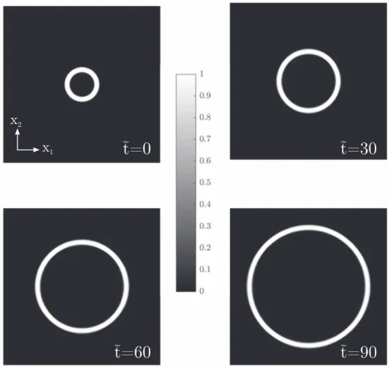
4.4.1. Smooth circular dislocation loop. Here we focus on the process of expansion of a smooth circular dislocation loop (see figure 4). This example was also investigated in

previous works where important spreading and damping was observed.

The initial dislocation density, characterized by a0 = a + a =3.5´ 110 2 120 2

( ) ( )  

107_m−1_{and represented infigure4, is again embedded in a uniform velocityfield v}

0=−1.

Figure 4. Mechanism of expansion of a circular dislocation loop. (a) Discrete dislocation line,(b) 3D density of dislocation, (c) 2D problem considered.

The unit-cell is discretized on a regular grid of 512×512 pixels, so the spatial scale is Δx=0.62b, (or D =x˜ 0.62). The CFL number considered is still

D D = v t x 0.25 68 0 1 ∣ ∣ ˜ ˜ ( )

so the dimensionless time step is D »t˜ 0.16, or equivalently D »t 1.44´10-14 _s. The results are represented infigure5at several time steps. The mechanism of expansion is well reproduced by the scheme and, again, the dislocation density is transported without any damping and spreading, in contrast with previous works.

4.4.2. Polygonal dislocation loop. We continue with the case of a dislocation loop with corners as defined in figure6. This is an interesting case because it admits non-unique weak solutions (Acharya 2003). In particular, following the comments of Varadhan et al (2006),

some entropy condition needs to be specified in order to choose between the so-called

Figure 5.Evolution of the dislocation density a a0 max

    in the process of expansion of a smooth circular loop.

expansion fan solution (a moving corner turns into an arc of constant radius) or the shock solution(a moving corner remains sharp).

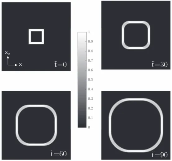
First, we consider the case of expansion of the polygonal loop, which corresponds to a uniform velocity v0=−1. The parameters considered in section 4.4.1are again used. The

mechanism of expansion is well reproduced in figure 7 by the scheme without notable damping and spreading. The corners do not stay sharp which means that the scheme automatically chooses the expansion fan solution. It should be noted that if the process is reversed at the end of the expansion by imposing v0=+1, the dislocation loop takes its

initial polygonal shape.

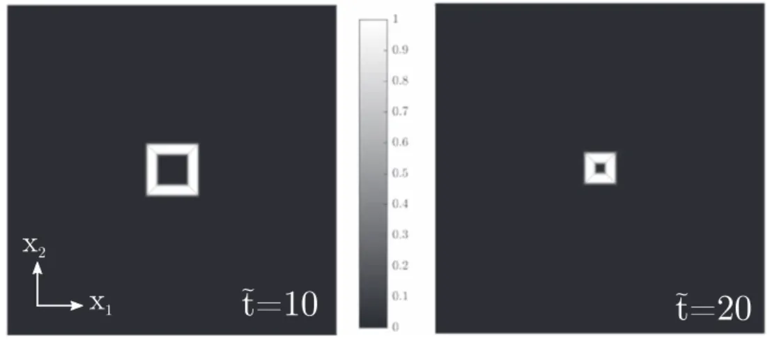
Then, we consider the case of shrinkage of an initially polygonal loop (defined in figure6), which corresponds to a uniform velocityv0=1.(Again, the same other parameters are considered.) The mechanism of shrinkage is well reproduced in figure 8 by the scheme without regularizing the corners as in the expansion process.

4.5. Discussion

As shown in section4.1, the transport of a modeled by equation(56) is conservative in

the velocityfield considered, which means that no damping and no spreading of a should be observed. The numerical scheme considered in this work has permitted to respect this property. The present results thus improve the prediction of dislocation motion formulated in the FDM framework in a simplified case where the plastic distortion tensor reduces to one component; indeed previous works suffer, in the same simplified problem, from numerical discrepancies such as oscillations, spreading and damping of dislocation den-sities. It is pointed out that predicting correctly the dislocation density motion is of the highest importance in coupled problems where the magnitude of the dislocation density will determine the stress level. In particular, an inaccurate transport of the dislocation density with damping, spreading and oscillations would induce spurious errors in the predictions of the stress and thus a poor prediction of the elastoplastic mechanical behavior.

5. Numerical results: coupled problems 5.1. Preliminaries

The aim of this section is to study numerically the evolution of the pointwise dislocation density tensor by considering the simplified FDM layer problem defined in section 3.2with no a priori assumptions on the velocity of dislocations v0: the stressfield is neither constant

nor uniform and the stress threshold is strictly positive; the evolution equation(51) is coupled

to the static problem(relations (18) and (19)).

In the sequel, we consider several 3D microstructures since the static problem is solved on a 3D cell made of elastic regions and a layer governed by FDM equations; in all cases, the unit-cell of 320b×320b×320b is discretized on a regular grid of 256×256×256 pixels, so the spatial scale isΔx=3.58×10−1nm. The thickness h of the layer is chosen to be very small (h=5b) so that the layer may be seen as a slip plane. This permits to reduce the possible fluctuation of the stress σ13 in the x3-direction so that the average stress τ13 is

very close to the stressσ13. Again, material data corresponding to aluminum are considered

Figure 7.Evolution of the dislocation density a a0 max

    in the process of expansion of a polygonal loop.

(see section 4.2). The parameters for the non-convex energy function are taken as follows:

β=10−8_andτ

y=1 MPa. The value of the threshold τyhas been taken to coincide with the

Peirls stress of aluminum (Kamimura et al2013).

Dislocation microstructures(such as a dislocation dipole for instance) produce initially an internal stressfield (Brenner et al2014). Thus, an initial microstructure can evolve without

any macroscopic stressfield applied, due to the local stress field produced by the dislocation density. Consequently we first need to study the possible equilibrium aspects of initial dis-location densities before any mechanical macroscopic loading. It should be noted that, in absence of lattice friction effects, initial microstructures will evolve and the dislocation will spread(Zhang et al2015); thus equilibrium positions of dislocation field may be allowed only

by the introduction of nonconvex energy density functions (Zhang et al 2015). In order to

investigate the possible equilibrium of the initial dislocation density field, we study its evolution while keeping a macroscopic zero stress field. Thus, the cell is subjected to a macroscopic loading pathe¯13 given by

e = U

2 , 69

13 13

p

¯ ⟨ ⟩ ( )

which imposes that the stress s¯13 is nil. Then, when the microstructure stops evolving, an equilibrium position is reached.

Equilibrated microstructures are then subjected to a mechanical loading in order to investigate the evolution of the dislocation density field. An increasing macroscopic strain e¯13=e¯˙13t is applied. The strain rate e¯˙13 is chosen low enough so the evolution may be considered as rate-independent.

5.2. Evolution of a dislocation loop

We consider the previous case of a circular dislocation loop. The initial dislocation density is characterized by a0 = a + a = 10 11 0 2 12 0 2 3 ( ) ( )

  m−1 and is represented in figure4. The CFL number considered is

Figure 8.Evolution of the dislocation density a a0 max

    in the process of shrinkage of a polygonal loop.

D D = v t x 0.25, 70 0 1 ∣ ∣ ˜ ˜ ( )

where the celerity of dislocation = t -t h

b

v0 cos U13 y 13

p

( )

( ˜ ˜ ) ˜ depends on the stress level. The time stepΔt is adjusted to ensure the value of the CFL number.

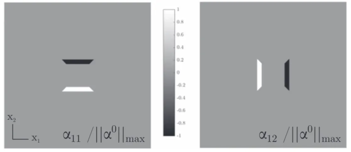
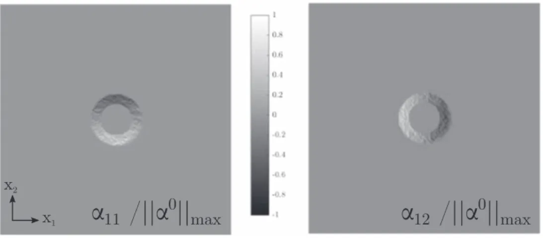
First we let the initial microstructure evolve in order to study its possible equilibrium position. The simulation reveals that the dislocation densityfield slightly oscillates around an equilibrium position that is represented infigure9. It is interesting to note that the dislocation field is somehow ‘noisy’ after this equilibrium process. This is due to the fact that the mobility of dislocations oscillates very rapidly in space around the value zero, due to the non-convex energy contribution which implies an alternation of positive, negative and zero velocity.

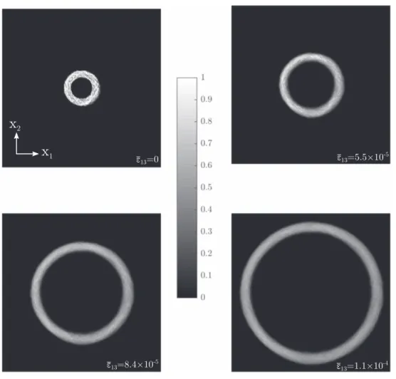
The equilibrated microstructure represented infigure9is then subjected to an increasing macroscopic strain. The results are represented in figure 10 at several strains: e = 0¯13 , e =_5.5´₁₀

-13 5

¯ ,e =¯13 8.4´10-5and e =¯13 1.1´10-4. The increase of the total straine¯13 induces an expansion of the circular loop which is due to an increase of the local stressfield. In contrast with the uncoupled problem, the velocity of the dislocation is not prescribed here and is only a consequence of the local mechanical state induced by the macroscopic straining and the dislocation density. It is interesting to note that the noisy effect observed in the equilibratedfield disappears during the loading because lattice effects are less dominant when the dislocation starts moving. It is worth noting that the dislocation remains compact during the evolution.

5.3. Orowan’s mechanism

As a second example we investigate the interaction between a dislocation loop and a pre-cipitate, which is known as Orowan’s mechanism. This mechanism consists in the formation of residual dislocation loops after the bowing of a dislocation around a precipitate. Such mechanism has important consequences on the strength of metallic alloys (i.e. precipitation hardening). In order to account for the presence of particles, we consider a heterogeneous distribution of the viscous drag coefficient η. We assume here that particles do not allow the motion of dislocations so they can be modeled by an infinite value of η which implies that the dislocation velocity (14) is zero. Two initial distributions are considered, one with dual

symmetrical precipitates (see figure 11(a)) and the second with a random distribution of Figure 9.Distribution of the dislocation density after equilibrium.

Figure 10.Evolution of the dislocation density a a0 max

    of an initially circular loop subjected to an increasing macroscopic strain.

Figure 11. Distribution of the viscous drag coefficient η in the case of (a) dual

symmetrical precipitates and(b) a random distribution of precipitates. The white color corresponds to h = ¥ and the black color corresponds toη=105Pa s m−1.

precipitates (see figure 11(b)). We consider as before a circular dislocation loop whose

equilibrium position is given infigure9.

The equilibrated microstructure is then subjected to an increasing macroscopic straine¯ .13 In the case of dual symmetrical precipitates, the results are represented infigure12at several strains: e =¯13 5.5´10-5, e =¯13 8.4´10-5, e =¯13 1.1´10-4 and e =¯13 1.2´10-4. The simulations show that the dislocation loop cuts itself in two parts while it gets around the precipitate. Once the precipitate is passed, the two parts of the dislocation density merge and form again a loop. After this process, a residual dislocation loop remains around the precipitate.

In the case of a random distribution of precipitates, the results are represented infigure13

at several strains:e = 0¯13 (equilibrium), e =¯13 5.5´10-5,e =¯13 8.4´10-5and e =¯13 1.1´

-10 4_{. The simulations show that the dislocation loop gets around each precipitate with the} same mechanism and a residual dislocation density remains around each precipitate.

Figure 12.Evolution of the dislocation density a a0 max

    of an initially circular loop subjected to an increasing macroscopic strain in the case of dual symmetrical precipitates.

5.4. Random microstructures

Wefinally investigate the possible emergence of spatial inhomogeneity of the Nye dislocation field (i.e. dislocation patterning). To do so, we consider the equilibrium and evolution of initially random distributions of the plastic distortion U₁₃p. A first microstructure (micro-structure A) is generated in the plastic layer using a random number generator which ensures that a0 = 10

max 3

  m−1andU13=0

p _{(see figure14(a)). Since the random number generation} is done in each pixel, the distribution ofU₁₃p is noisy, which may induce damping during the evolution problem. Thus, a second microstructure is generated by applying a smoother (Garcia2010) which permits to keep the same properties ( a0 = 10

max 3

  m−1andU₁₃p =0) while gaining in smoothness(see figure14(b)). The aim of this study is only to illustrate the

possible emergence of patterning, so no attempt is done here to characterize thoroughly these microstructures in terms of morphology and representativity(Jeulin2012).

Figure 13.Evolution of the dislocation density a a0 max

    of an initially circular loop subjected to an increasing macroscopic strain in the case of a random distribution of precipitates.

Microstructure A. First we let the‘noisy’ random microstructure evolve in order to study its equilibrium position. The dislocation density reaches an equilibrium position(see figure15

upper left snapshot) consisting in an organized lamellar microstructure mimicking tortuous dislocation cells. The value of the dislocation density a is ten times lower than its initial value, due to an important damping. (The evolution of a is not conservative since the hypotheses of section4.1are not met in the coupled case.) The equilibrated microstructure is then subjected to an increasing macroscopic straine¯ . The results are represented in13 figure15 at several strains: e = 0¯13 (equilibrium), e =¯13 1.3´10-5, e =¯13 2.2´10-5 and e =₃ ´₁₀

-13 5

¯ . The ‘lamellar’ microstructure is followed by a ‘globular’ microstructure made of dislocation loops separated by thin walls. This type of microstructure evolution, obtained from a random distribution of plastic distortion, resembles the formation of dis-location cells. This apparent disdis-location patterning seems very similar to the formation of crystal grains. However, the cells boundaries do not act here as classical grain boundaries where dislocation loops can stack up. Indeed, if the loading is increased, dislocations loops will continue interacting and will annihilate in absence of dislocation nucleation and no pile-up is observed.

Microstructure B. Then we consider the case of the‘smooth microstructure’. Again, the dislocation density reaches an equilibrium position (see figure 16upper left snapshot) con-sisting in an organized lamellar microstructure. The initial cells are more apparent due to a bigger size. It is worth noting that no damping of a is observed, in contrast with the noisy microstructure. The equilibrated microstructure is then subjected to an increasing macro-scopic straine¯ . The results are represented in13 figure16 at several strains:e = 0¯13 (equili-brium), e =¯13 1.3´10-5, e =¯13 2.2´10-5 and e =¯13 3 ´10-5. Again, the ‘lamellar’ microstructure is followed by a‘globular’ microstructure made of dislocation loops separated by thin walls. In that case, the formation of dislocation cells is more patent because they are bigger. This microstructure is very similar to crystal grains in which dislocation loops grow. Again, no pile-up is observed due to dislocation annihilation between loops of neighboring cells.

Figure 14.Distribution of the initial plastic distortion U13 U p

13,max p

.(a) Noisy random microstructure (microstructure A), (b) smoothed random microstructure (microstruc-ture B).

In both cases, it is worth noting that strain unloading, up to a nil macroscopic stress, permits to stop the evolution of the microstructure and thus leads to a stabilization of the pattern.

6. Conclusion

The aim of this work was to investigate dislocation-mediated plasticity using the FDM theory. First, the mesoscale FDM theory was recalled which has permitted to clearly identify two distinct problems to be solved, the static problem consisting in the determination of the local stress field for a given dislocation density (elliptic equation), and the evolution problem consisting in the transport of the dislocation density (hyperbolic equation). An efficient numerical integration procedure was then proposed. The static problem was solved in a general case using the FFT-based scheme proposed by Brenner et al 2014. The evolution problem, consisting in a vectorial tridimensional Hamilton–Jacobi hyperbolic equation, was

Figure 15. Evolution of the dislocation density a a0 max

    of an initially noisy random microstructure (microstructure A) subjected to an increasing macroscopic strain.

solved in a simplified layer case using a high resolution Godunov-type scheme. Model problems werefinally considered in order to investigate the predictions of the theory. First, uncoupled problems with constant velocity were explored: the numerical scheme considered has permitted to reproduce accurately physical phenomena such as the annihilation of dis-locations and the expansion of a dislocation loop. Then, the FDM theory was applied to coupled problems in order to investigate several problems of dislocation-mediated plasticity. In a model problem of interactions between a dislocation and precipitates, the formation of residual dislocation loops around the precipitates has been observed. Finally, the evolution of random microstructures has been studied as a possible way to access dislocation patterning. The present work permits to confirm the expectations funded in the FDM theory for predicting several mechanisms of dislocation-mediated plasticity(Acharya2010). The present

formulation is not complete since only one component of the plastic distortion tensor was considered. Future developments concerning the numerical integration of the 3-d FDM theory are thus necessary to tackle more general problems of plasticity. A future important task will

Figure 16.Evolution of the dislocation density a a0 max

    of an initially smooth random microstructure (microstructure B) subjected to an increasing macroscopic strain.