Bibi : CIRPÉE, Pavillon DeSève, Université Laval, Québec, Canada G1V 0A6
sbibi@ecn.ulaval.ca
Makdissi : Department of Economics, University of Ottawa, 55 Laurier E. (10125), Ottawa, Ontario, Canada K1N 6N5
paul.makdissi@uottawa.ca
Yazbeck: Département d’économique and CIRPÉE, Pavillon DeSève, Université Laval, Québec, Canada G1V 0A6
myazbeck@ecn.ulaval.ca
We thank Raymond Kmeid, vice-president SNAM, S.A.L., for providing us with valuable information on the Lebanese housing
Cahier de recherche/Working Paper 09-39
Equivalence Scales and Housing Deprivation Orderings: an Example
Using Lebanese Data
Sami Bibi Paul Makdissi Myra Yazbeck
Abstract:
Housing deprivation orderings raise challenges as far as measurement is concerned. The first challenge resides in the identification of an adequate variable that characterizes housing services consumed by households. Another challenge may arise in the comparisons of housing services consumption between households of different sizes and composition. The last challenge may arise in the choice of a deprivation threshold and of a deprivation index. In this paper we address theoretically those challenges. An empirical illustration is offered using Lebanese data.
Keywords: Housing, Deprivation, Stochastic dominance, Equivalence scales, Lebanon
The States Parties to the present Covenant recognize the right of everyone to an adequate standard of living for himself and his family, including adequate food, clothing and housing, and to the continuous improvement of living conditions.
[International Covenant on Economic, Social and Cultural Rights, UN]
1 Introduction
Adequate housing is considered as one of the basic needs and a human right. When comparing the extent to which different groups of households are able to meet such basic needs, an analyst faces three main problems. The first problem is the identification problem. In order to identify those who do not meet their basic needs, the analyst must select an adequate threshold under which basic needs are considered not met. In this context, the selection of an adequate variable that char-acterizes housing services consumed by households remains difficult. The surface of the dwelling in square meters (m2) may be an appealing indicator, however it can be argued that housing quality, proximity to services and location may not be captured by its surface. In this paper, we rely on the market value as it provides a better indicator of housing quality.
The second problem lies in the choice of the aggregation procedure. The an-alyst must select an adequate index to transpose household’s or individual’s de-privation into an aggregate measure. The most commonly used income poverty indices are the FGT poverty measures (Foster, Greer, and Thorbecke, 1984), but other measures can be used as well. The FGT measures can also be applied to other indicators of wellbeing such as child malnutrition or housing deprivation (see among others Bourguignon and Chakravarty, 1999). To test whether the de-privation ordering depends on the choice of the dede-privation index, analysts often perform stochastic dominance tests to ensure that the comparisons remain valid
for a wide spectra of deprivation indices and deprivation thresholds (see Atkinson, 1987, Zheng, 1999, Zheng, 2000 and Duclos and Makdissi, 2004).
The last problem relates to the heterogeneity in households’ needs. When comparing income deprivation between households of different sizes, analysts usually select an equivalence scale that transforms household income into an equivalent income. The use of an equivalence scale is motivated by the existence of economies of scale in household consumption. Given that such economies of scale exist in the case of housing, household needs do not increase in the same proportion as household size. In the context of income poverty, Buhmann, Rain-water, Schmaus and Smeeding (1987) empirically show the importance of the impact of different equivalence scale elasticities on poverty measurement. They use a simple parametric equivalence scale based on household size. Subsequently, Coulter, Cowell and Jenkins (1992b) use similar parameterization and analyze the theoretical impact of marginal changes in the equivalence scale’s elasticity on poverty measurement (see also Coulter, Cowell and Jenkins, 1992a). Also, Banks and Johnson (1994), Jenkins and Cowell (1994) and Duclos and Mercader (1999) generalize this approach for a class of parametric equivalence scales that are extended to take into account household composition. These papers, along with those of Phipps (1991), Burkhauser, Smeeding and Merz (1996), and De Vos and Zaidi (1997), find that international comparisons of poverty and poverty profiles are strongly influenced by the assumptions made on household needs. In this paper, we test (among other things) whether or not the ordinal comparisons of housing deprivation are robust to the selection of the equivalence scale’s elasticity. The objective of this paper is twofold. First, it aims at analyzing the mea-surement difficulties inherent to housing deprivation comparisons. It also offers an illustration by comparing housing deprivation among demographic groups in Lebanon. Second, it addresses the equivalence scale problem. In a first step, we
use Coulter et al. (1992b) framework for analyzing the impact of the equivalence scale elasticity on FGT comparisons. We extend their theoretical result to account for the impact of the equivalence scale elasticity on stochastic dominance com-parisons. We then apply this framework to housing deprivation comparisons in Lebanon. In this paper, we adopt a market value approach as an indicator of hous-ing services. To compute the market value of houshous-ing services for households who own their dwelling, we use the usual hedonic prices models. One major difficulty arises given the presence of an old Lebanese law that prohibits rent increase on old rent contracts. The presence of such a law implies that some tenants may enjoy an in kind subsidy of rent.
The remainder of the paper is organized as follows. Section 2 presents the theoretical framework, Section 3 displays our empirical analysis of housing de-privation in Lebanon and Section4concludes.
2 Theoretical framework
2.1 Parametric equivalence scales
To perform welfare comparisons across household with different needs, it is a common practice to use an equivalence scale to transform household’s income into an equivalent income. The theoretical argument is based on the existence of economies of scale in household consumption. A larger household may thus need a lower level of per capita income in order to achieve the same level of welfare than a smaller household. This argument is particularly valid in the context of comparisons of housing services enjoyed by different households. In our context, the equivalence scale transforms the observed value for total housing services, x, into equivalent housing services, y.
list thirty-four different equivalence scales in their paper1. To analyze the different equivalence scales, Buhmann et al. (1987) also introduce the following parametric form
m (n) = nθ, (1)
where n is the household size, m (n) is the equivalence scale and θ is the equiva-lence scale elasticity. In the context of housing services, equivalent housing ser-vices are defined by
y = x
m (n), (2)
In this setting, the equivalence scale elasticity, θ, is theoretically expected to vary between 0 and 1. When the equivalence scale elasticity is equal to 1, housing ser-vices are considered as private good and there are no economies of scale. How-ever, if the equivalence scale elasticity is 0, housing services are considered as a pure public goods and there is no welfare cost of adding one person to the house-hold. For all values between 0 and 1, we consider that there exist some economies of scale in housing services. In practice, the equivalence scale elasticities vary over almost all the theoretical interval. In the context of equivalent income, the thirty-four equivalence scales presented in Buhmann et al. (1987) vary between 0.12 and 0.84.
2.2 Housing deprivation indices and ordering
The objective of this section is to describe the theoretical setting in which we perform our analysis. In order to perform our analysis, we need to partition the population set in different family types or regions. Therefore, we will consider only additive deprivation measures. Let F : <+→ [0, 1] represents the cumulative
distribution of equivalent housing services y. In this framework total housing
deprivation is given by DF(z) = Z z 0 δ (y, z) dF (y) , (3) where: δ (y, z) ≥ 0, if y ≤ z, δ (y, z) = 0, if y > z. ¾ (4) Here z, is the threshold under which a household is considered deprived in the dimension of housing services. The function δ (y, z) represents the contribution to total deprivation made by a household enjoying equivalent housing services
y. A popular class of additive poverty indices that can be used in the context of
housing deprivation is the class of FGT indices, defined as
F GTF(α, z) = Z z 0 µ z − y z ¶α dF (y) . (5)
Other examples of additive indices are the Chakravarty (1983) poverty indices and the Watts (1968) index that is defined as
W =
Z z 0
log (y/z) dF (y) , (6)
which can in turn be seen as a transformation of Clark, Hemming and Ulph’s (1981) second class of poverty indices. In this paper, we choose the FGT class of deprivation indices. However, we also perform stochastic dominance tests to ensure that our results remain robust to a change in the deprivation index. To do so, we regroup these additive indices into classes Ξs, s = 1, 2, . . . , of deprivation indices. These classes are defined by:
Ξs := D ¯ ¯ ¯ ¯ ¯ ¯ δ(y, z) ∈ bCs(z),
(−1)iδ(i)(y, z) ≥ 0 for i = 0, 1, ..., s,
δ(t)(z, z) = 0 for t = 0, 1, ..., s − 2
, (7)
where bCs(z) represents the set of functions that are s times piecewise differen-tiable on [0, z)2. δ(i)(y, z) represents the i-th derivative of δ (y, z) with respect of
2Notice that if the (s − 1)-th derivative of a function is piecewise differentiable, the (s − 1)th
its first argument.
At this point, it is useful to supply a normative interpretation of the different classes of indices. When s = 1, the indices must be such that housing deprivation weakly decreases when a household’s housing services increase. These indices are thus of the Pareto type in addition to being symmetric in income (they obey the anonymity axiom). When s = 2, these indices respect the Pigou-Dalton principle of transfers. This principle postulates that a mean-preserving transfer of hous-ing services from a higher-level of houshous-ing services household to a lower-level of housing services household constitutes a social improvement. When s = 3, the indices are also sensitive to favorable composite transfers. These transfers are such that a beneficial Pigou-Dalton transfer within the lower part of the distribu-tion, accompanied by a reverse Pigou-Dalton transfer within a higher part of the distribution, will decrease deprivation provided that the variance of the distribu-tion is not increased. Kolm (1976) was the first to introduce this condidistribu-tion into the inequality literature, and Kakwani (1980) subsequently adapted it to poverty mea-surement (see also Shorrocks and Foster (1987) for a complete characterization of this transfer principle). For the interpretation of higher orders of dominance, we can use the generalized transfer principles of Fishburn and Willig (1984). For
s = 4, for instance, consider a combination of composite transfers, the first one
being favorable and occurring within the lower part of the distribution, and the second one being unfavorable and occurring within a higher part of the tion. Because the favorable composite transfer occurs lower down in the distribu-tion, indices that are members of the s = 4 classes should respond favorably to
continuous and differentiable everywhere. Note that the continuity condition we impose is more restrictive than that in Zheng (1999), which only postulates continuity on the interval [0, z) without
any restriction on δ(t)(z, z) = 0 for t = 0, 1, ..., s − 2. This difference between his and our
assumptions has implications for the analysis developed in this paper. Specifically, we are able to consider dominance criteria for orders greater than two, even when there is significant uncertainty on the value of the lower bounds for the ranges of possible deprivation thresholds. For details, see Duclos and Makdissi (2004).
this combination of composite transfers. Generalized higher-order transfer princi-ples essentially postulate that, as s increases, the weight assigned to the effect of transfers occurring at the bottom of the distribution also increases. Blackorby and Donaldson (1978) describe these indices as becoming more Rawlsian. As shown in Davidson and Duclos (2000), when s → ∞ only the lowest level of housing services counts.
In this theoretical setting, Atkinson (1987) has developed stochastic domi-nance conditions that enable us to identify deprivation orderings that are valid for all indices in the Ξ1 and Ξ2 classes. Duclos and Makdissi (2004) generalize these conditions for all classes Ξs. Consider two equivalent housing services dis-tribution functions, F and G. For expositional simplicity, we define stochastic dominance curves F1(y) = F (y) and Fs(y) = Ry
0 Fs−1(u) du for all integers
s ≥ 2. Gs(y) is defined analogously. When deprivation does not increase in a movement from distribution F to distribution G, we have that:
∆DAF G(z) = Z a 0 δA(y, z) dG (y) − Z a 0 δA(y, z) dF (y) ≤ 0. (8) If there is a consensus that the deprivation threshold z should not exceed some maximum, denoted by z+, then it is possible to lay out a necessary and sufficient condition for absolute deprivation dominance applicable to all orders of stochastic dominance. In this framework, Duclos and Makdissi (2004) show that deprivation does not increase in a movement from distribution F to distribution G, for all deprivation indices D ∈ Ξsand all deprivation thresholds z ∈ [0, z+] if and only if
Fs(y) − Gs(y) ≥ 0 for all y ≤ z+. (9)
If the stochastic dominance test fails at order s, two different strategies may be followed. The first increases the order of stochastic dominance until a depriva-tion ordering becomes robust over all of some pre-specified ranges of deprivadepriva-tion
thresholds. Davidson and Duclos (2000) have shown that if there is dominance in the lower part of the distribution then, for some higher order of stochastic dom-inance we will find domdom-inance over all [0, z+]. The second strategy consists in inferring a critical bound for a restricted range of deprivation thresholds. This critical deprivation threshold zs beyond which (9) does not hold anymore is then given by
zs= sup {z |Fs(y) ≥ Gs(y) , y ∈ [0, z]} . (10)
2.3 The impact of the equivalence scale’s elasticity on
depriva-tion indices and orderings
The aim of this section is to analyze the theoretical impact of the equivalence scale’s elasticity on deprivation indices and orderings. Assume that there are N different household sizes and that households only differ in their size. For each household size n, we have a housing services distribution function Fn(x) where
x = m (nn) · y. In this framework, we can write
F GTF (α, z) = N X n=1
πnF GTFn(α, zn) (11)
where zn = m (n) · z and πnrepresents the population share of households of size
n. In such a framework, Coulter et al. (1992b) showed that ∂F GTF (α, z) ∂θ = ( PN n=1πnznln (n) fn(zn) if α = 0 PN n=1πnln (n) α Rzn 0 ³ zn−x zn ´α−1³ x zn ´ dFn(x) if α ≥ 1 (12)
Equation (12) allows us to conclude that an increase in the value of the equiv-alence scale elasticity induces an increase of housing deprivation, F GTF (α, z). This increase may be decomposed into two effects. The first effect given by
znln (n), is what Coulter et al. (1992b) called a pure poverty line effect (de-privation threshold in our context). A higher θ implies a higher equivalence scale
for all household types (bar singles), thus a higher deprivation threshold. Given that these deprivation thresholds are defined in terms of observed housing ser-vices, which remain unchanged with a variation of the equivalence scale, more households will be deprived. The second effect flows through the change of the equivalent housing services distribution at the deprivation threshold. For α = 0, this effect is given by the density at the deprivation threshold. For α ≥ 1, this impact is given by theRzn
0 ³ zn−x zn ´α−1³ x zn ´ dFn(x)’s.
To transpose Coulter et al. (1992b) result to robust orderings, we must assess the impact of a change in the equivalence scale elasticity on stochastic dominance curves. Stochastic dominance tests provide ordinal rankings of alternatives. Con-sequently, one might be inclined to think that analyzing the impact of marginal changes of the equivalence scale elasticity on the cardinal position of the stochas-tic dominance curves is not interesting per se. However, this overlooks the inter-est of analyzing the impact of such a marginal change on the value of the critical deprivation threshold, zs. It is important to note that this critical threshold is a useful tool when stochastic dominance tests fail to provide a robust ordering for
z ∈ [0, z+]. To analyze the impact of marginal changes in θ, it is convenient to decompose stochastic dominance curves into subgroups.
Fs(zs) = N X n=1
πnFns(zns) (13)
Standard calculus enable us to find that
∂Fs(zs) ∂θ = ½ PN n=1πnznln (n) fn(zsn) if s = 1 PN n=1πnznln (n) Fns−1(zns) if s ≥ 2 . (14)
Analogous results may be obtained for ∂Gs(zs)/∂θ. Looking at equation (14) leads us to conclude that an increase in the value of the equivalence scale elasticity induces an increase of the value of Fs(zs). As for F GT indices, this increase may be decomposed into two effects. The pure poverty line effect is given by znln (n).
The second effect flows through the change of the equivalent income distribution at the critical poverty threshold. For s = 1, this effect is given by the density at the poverty line. For s ≥ 2, this impact is given by the Fs−1
n (zsn)’s.
Given this analytical result of the impact of a marginal change of θ on stochas-tic dominance curves, we can find the impact of these variations on the cristochas-tical poverty threshold. Since, by definition, Fs(zs) = Gs(zs), the sign of the varia-tion of zswill be given by the difference between the variation of Fs(zs) and the variation of Gs(zs). Explicitly, we have
∂zs ∂θ ≶ 0 ↔ ∂Fs(z) ∂θ − ∂Gs(z) ∂θ ≶ 0. (15)
3 Housing deprivation in Lebanon
3.1 The Lebanese Context: Housing Sector and Data
Descrip-tives
In this paper, we use data from the Population and Household Survey (PHS) conducted by the Ministry of Social Affairs of Lebanon in 1996. Before analyzing the data, it is worth to describe the Lebanese housing sector and give a brief histor-ical perspective on the value of the Lebanese pound. The Lebanese housing sector is characterized by an old rent control law that prohibited rent increases (in nomi-nal terms) and expulsion. In such a context, the tenant had a quasi-property right on the dwelling. This kind of regulation induces strong rigidities on the housing market. These rigidities coupled with a strong devaluation of the Lebanese pound in the 80’s lead to an unsustainable situation in which it was merely impossible to find a new dwelling on the formal housing market. During the first part of the civil war in Lebanon, the Lebanese pound managed to maintain its value in term US dollars between 0.33 and 0.25. However, after the first Israeli invasion of Lebanon
in the summer of 1982, the Lebanese pound started to quickly depreciate3. In the following 10 years, the pound devaluated to 0.000396 US dollars, which is a little bit less than 0.12% of its value at the beginning of the civil war. Nowadays, the value of the Lebanese pound worth 0.000663 US dollars. In this context of rapid devaluation, the rent control law had strong redistributive impact from landlord to tenant. People refused to rent dwellings. Dwelling rental became an informal activity; people tried to avoid the rent control regulation using informal contracts. All this lead to a legal reform that partially liberalized the housing market in 1992. The 159/92 act created the possibility of fixed term renting contract for a period of three years with a 10% rent increase every year (or any other amount agreed upon between the two parties). Under the 160/92 act, people with old rents were still protected against nominal rent increases.
The PHS is a nationally representative household survey with the exception of some occupied territory for which the Lebanese civil servants did not have access at that time. The sample consists of 61,150 households. The questionnaire has information on housing ownership, the rent paid as well as on the dwelling’s characteristics. This information is used to obtain measures of housing quality based on imputed rental values.
The indicator of housing quality used in this paper is obtained from a standard hedonic regression of rental values for household with rent contracts signed after 1992. The vector of dwelling characteristics includes the district location; whether the dwelling is in an urban or rural area; the type of housing, namely, whether it is a house or apartment, a shack, a mobile home; the number of rooms; the type of heating system, namely combustible fuel, central, electric or else; the type of access to water, namely municipal network, private network; the type of access to drinking water, namely network with no purification, network with purification,
3We do not assume nor refute that this invasion is the principal causal factor of the depreciation
spring source, bottled water or other, the type of sewage system, namely public sewage, open sewage, sceptic sewage, and the number of telephone line in the dwelling.
Table1displays the hedonic regressions results. The basic idea behind the use of these regressions is that rents should broadly reflect rental values, i.e. house-holds willingness to pay for different quality levels. For househouse-holds who do not pay a market value rent4, we use a prediction of the rental value as an indicator of housing quality5. Also, for households with a per capita rental value lower than 1% of the mean per capita rental value, we apply a bottom coding procedure that imputes to these observations a rental value equal to this threshold.
Using this information, we compare housing deprivation of different regions and demographic groups: (1) Beirut vs Mount Lebanon and Bekaa, (2) nuclear families vs other families and (3) families having members living abroad vs other families. Note that we exclude from the regional comparisons North Lebanon, South Lebanon and Nabatieh. These regions have experienced low construction activities in the year following the civil war because of instability. In this case, the rents paid do not adequately reflect housing quality. Using imputed rental value of the household’s dwelling, we test whether one group is more likely to live in poor housing conditions than the other.
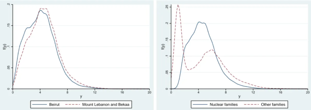
Figure1provides the density functions for housing rental values for the three comparisons. Two facts emerge from these figures. The first suggests that families living in Beirut are doing better than families living in Mount Lebanon and Bekaa. Also families having members living abroad are doing better than other families. While such an interpretation come in line with conventional wisdom, it could be
4They own their dwelling or they are provided with free housing or they have moved into their
rented dwelling prior to 1992.
5For 1.9% of total observations in the data set, we have a rent paid that exceeds the predicted
value from the regression even if the household had moved in prior to 1993. In those case we used actual rent paid as indicator of rental value.
misleading. In fact, these findings may be sensitive to the choice of the equiva-lence scale. We will test this possibility later in this section. The second suggests that there is no differences between nuclear families and other families in term of housing achievement. As we will see later, in this particular case, accounting for economies of scale may change this finding.
In Figure2, we provide densities of household sizes. It is clear that families living in Beirut tend to be smaller than families living in Mount Lebanon and the Bekaa. Similarly, families having members living abroad tend to be smaller than other families. In these two cases, family size may reinforce the fact that families living in Beirut and families having members living abroad are doing better than the others. More interesting case is the comparison between nuclear families and “other” families. Surprisingly, “other” families have a bimodal density of house-hold size. This can lead to interesting results when introducing the equivalence scale in the comparisons.
3.2 Deprivation Analysis
To identify the poor, we fix the deprivation threshold to half of the mean per capita rental value for households of size 4. This deprivation threshold takes a value of 348,000 Lebanese pounds. In the remainder of the paper, we will nor-malize rental values by this per capita deprivation threshold. In this context, a value of 1 (100%) is associated with 348,000 pounds and a value of 2 (200%) with 698,000 pounds.
Table2displays the estimates of household deprivation indices for the country. As expected, deprivation estimates increase with the elasticity of the equivalence scale. It is important to emphasize that, even if we were confident that our he-donic regression model gives an exact picture of the value of housing services, the measurement difficulty associated with the choice of an equivalent scale
re-mains important. We can see in Table2that for the selected deprivation threshold, poverty incidence varies between 2.14% (for θ = 0) to 21.98% (for θ = 1). Table
3displays the derivatives of deprivation indices. The derivatives seems to be con-sistent with the increases in estimates. The larger is the derivative in one point, the larger is the increase in the estimate induced by an increase in the equivalence scale elasticity.
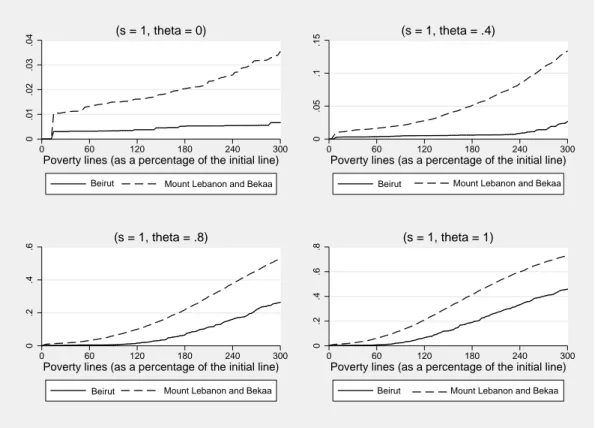
Focusing our attention on differences in deprivation among geographic areas, we try to determine the extent to which housing deprivation is lower in Beirut. Table 4 displays the estimates of deprivation indices for Beirut and for Mount Lebanon & Bekaa. It is obvious that for any values of α and θ, deprivation is lower in Beirut. Thus the impressions that we had while looking at the density curves of housing services and family sizes seems to be verified. In order to test whether or not this holds for a wider spectra of measurement assumptions, we perform stochastic dominance tests. For this purpose, we use a maximum deprivation threshold z+ = 300%6. If the stochastic dominance curves do not intersect before z = 300%, we obtain a robust ordering of deprivation for a given value of θ. Figure 3 displays first order stochastic dominance tests for various choices of θ. There is obviously less housing deprivation in Beirut than in the rest of the country and this conclusion seems to hold for any value of the deprivation threshold, any deprivation index and any value of the equivalence scale elasticity. Turning our attention to differences in deprivation among families with and without members living abroad, we try to answer another question: Are families with members living abroad less deprived in term of housing than other families? Table 5displays the estimates of deprivation indices for families with members living abroad and for other families. Looking at Table 5, we note that for any
6This maximum threshold is 1.5 times the mean per capita rental value for households of size 4.
Note that this maximum threshold is sufficiently large to include all possible deprivation threshold that one may think of.
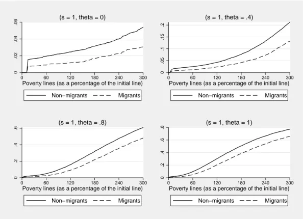
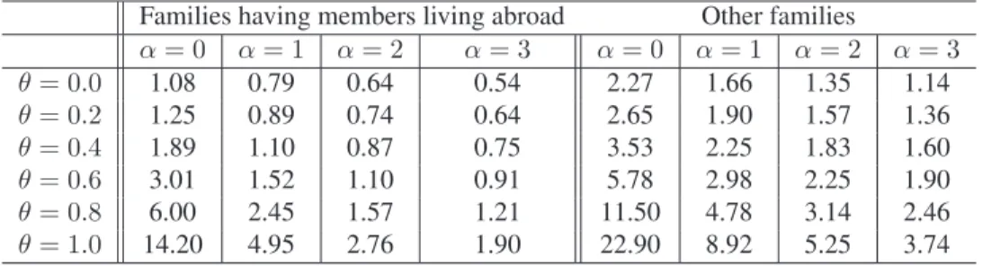
values of α and θ, deprivation is lower for families having member living abroad. Once again, the conclusion drawn from the density curves of housing services and family sizes seems to be verified. Also, we perform stochastic dominance tests to check for robustness in measurement assumptions. Figure4displays first order stochastic dominance tests for various choices of θ. Obviously, there is less housing deprivation for families having members living abroad. This conclusion seems to hold for any value of the deprivation threshold, any deprivation index and any value of the equivalence scale elasticity.
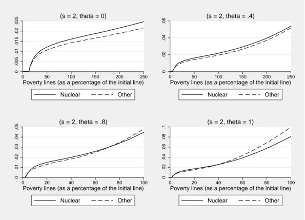
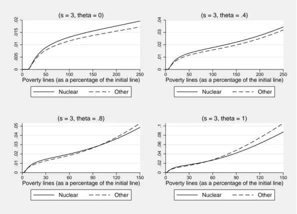
Finally, we consider differences in deprivation among nuclear families versus other families. Nuclear families are defined as families where we can find a father, a mother and/or children. Other families’ structure includes extended families as well as multi-families households. It is important to note that the comparison of these two demographic groups is interesting for methodological considerations. In fact, it helps us illustrate the measurement difficulties that can be associated with a change in measurement assumptions. Unlike the two previous comparisons, this comparison is not robust to a change in analytical assumptions. Table6displays the estimates of deprivation indices for nuclear families and other families. A first look at this table shows that the comparison of these two demographic groups depends on the measurement assumptions. For lower values of θ, nuclear families have higher deprivation indices and the opposite holds for higher values of θ. For intermediate values of θ, increasing aversion to poverty (α) seems to benefit other families. Figures 5, 6 and 7 display stochastic dominance tests of order 1 to 3 for this comparison. For low values of θ, nuclear families have a higher housing deprivation than other families and this ordering is robust. For θ = 0.8 and 1.0, the two stochastic dominance curves intersect at values that are lower than the initial poverty line. As mentioned earlier, two different strategies may be followed. Thus, one can increase the order of dominance to obtain a robust
ordering for all values of θ. Alternatively, one can estimate critical deprivation threshold, zsas defined in equation (10). Table7displays the value of zsfor the first four orders of stochastic dominance. We note that increasing the order of dominance to s = 4 produces a robust ordering of deprivation between the two demographic groups. Also, a complete ordering of these two groups for s = 1, 2 or 3 and any values of θ, may be obtained only at the cost of restricting the maximum poverty line to 26.1%, 39.5% or 53.1% for order 1,2 or 3 respectively. Table 8 displays the sign of ∂zs/∂θ at the intersection of stochastic dominance curves. For all intersections, this sign is negative. This is consistent with the fact that zsdecreases as θ increases as shown in Table7.
4 Conclusion
This paper has used Coulter et al. (1992b) framework to analyze the impact of changes in equivalence scale elasticity on housing deprivation indices in Lebanon. It has also built on this framework and on Duclos and Makdissi (2004) to ana-lyze the impact of changes in equivalence scale elasticity on stochastic dominance comparisons. This theoretical framework has been used to compare housing depri-vation between region and demographic group in Lebanon. Housing depridepri-vation appears to be lower in Beirut than in Mount Lebanon and Bekaa and lower for families having members living abroad that for the other families. These order-ings are robust to changes in measurement choices of the deprivation threshold, the deprivation index and the elasticity of the equivalence scale. The paper also shows that such an ordering is not obtained when we compare nuclear families to the other families and that the ordering of housing deprivation between these two demographic groups is contingent to measurement choices.
References
[1] Atkinson, A.B. (1987), On the Measurement of Poverty, Econometrica, 55, 759-764.
[2] Banks, J. and P. Johnson (1994), Equivalence Scale Relativities Revisited,
The Economic Journal, 104, 883-890.
[3] Blackorby, C. and D. Donaldson (1978), Measures of Relative Equality and Their Meaning in Terms of Social Welfare, Journal of Economic Theory, 18, 59-80.
[4] Bourguignon, F. and Chakravarty, S.R. (1999), A Family of Multidimen-sional Poverty Measures, in D. Slottje (ed.), Advances in
economet-rics, income distribution and scientific methodology: Essays in honor of Camilo Dagum, 331-344.
[5] Buhmann, B. , L. Rainwater, G. Schmaus and T.M. Smeeding (1987), Equiv-alence Scales, Well-Being, Inequality, and Poverty: Sensitivity Esti-mates Across Ten Countries Using the Luxembourg Income Study (LIS) Database, Review of Income and Wealth, 34, 115-142.
[6] Burkhauser, R.V., T.M. Smeeding and J. Merz (1996), Relative Inequality and Poverty in Germany and the United States Using Alternative Equiv-alence Scales, Review of Income and Wealth, 42, 381-400.
[7] Chakravarty, S.R. (1983), A New Index of Poverty, Mathematical Social
Sciences, 6, 307-313.
[8] Clark, S., R. Hemming and D. Ulph (1981), On Indices for the Measurement of Poverty, The Economic Journal, 91, 515-526.
[9] Coulter, F.A.E., F. A. Cowell and S. P. Jenkins (1992a), Differences in Needs and Assessment of Income Distributions, Bulletin of Economic Research,
44, 77-124.
[10] Coulter, F.A.E., F. A. Cowell and S. P. Jenkins (1992b), Equivalence Scale Relativities and the Extent of Inequality and Poverty, The Economic
Journal, 102, 1067-1082.
[11] Davidson, R. and J.Y. Duclos (2000), Statistical Inference for Stochastic Dominance and for the Measurement of Poverty and Inequality,
Econo-metrica, 68, 1435-1465.
[12] De Vos, K. and M.A. Zaidi (1997), Equivalence Scale Sensitivity of Poverty Statistics for the Member States of the European Community, Review of
Income and Wealth, 43, 319-333.
[13] Duclos, J.-Y. and P. Makdissi (2004), Restricted and Unrestricted Domi-nance for Welfare, Inequality and Poverty Orderings, Journal of Public
Economic Theory, 6, 145-164.
[14] Duclos, J.-Y. and M. Mercader-Prats (1999), Household Needs and Poverty: With Application to Spain and the UK, Review of Income and Wealth, 45, 77-98.
[15] Fishburn, P.C., and R.D. Willig (1984), Transfer Principles in Income Re-distribution, Journal of Public Economics, 25, 323-328.
[16] Foster, J.E., J. Greer and E. Thorbecke (1984), A Class of Decomposable Poverty Measures, Econometrica, 52, 761-776.
[17] Jenkins, S.P. and F.A. Cowell (1994), Parametric Equivalence Scales and Scale Relativities, Economic Journal, 104, 891-900.
[18] Kakwani, N. (1980), On a Class of Poverty Measures, Econometrica, 48, 437-446.
[19] Kolm, S.-C. (1976), Unequal Inequality: I, Journal of Economic Theory, 12, 416-442.
[20] Phipps, S.A. (1991), Measuring Poverty Among Canadian Households: Sen-sitivity to Choice of Measure and Scale, The Journal of Human
Re-sources, 28, 162-184.
[21] Shorrocks, A.F. and J.E. Foster (1987), Transfer Sensitive Inequality Mea-sures, Review of Economic Studies, 54, 485-497.
[22] Watts, H.W. (1968), An Economic Definition of Poverty, in D.P. Moynihan (ed.), On Understanding Poverty, Basic Books, New York.
[23] Zheng, B. (1999), On the Power of Poverty Orderings, Social Choice and
Welfare, 3, 349-371.
[24] Zheng, B. (2000), Poverty Orderings, Journal of Economic Surveys, 14, 427-466.
Figure 1: Comparisons of densities of rental values
Densities of rental values for Beirut vs Mount Lebanon and Bekaa
0 .00005 .0001 .00015 .0002 .00025 f(y) 0 4000 8000 12000 16000 20000 y
Beirut Mount Lebanon and Bekaa
Densities of rental values for nuclear families vs other families
0 .00005 .0001 .00015 .0002 .00025 f(y) 0 4000 8000 12000 16000 20000 y
Nuclear families Other families
Densities of rental values for nuclear families vs other families
0 .00005 .0001 .00015 .0002 .00025 f(y) 0 4000 8000 12000 16000 20000 y
Figure 2: Comparisons of densities of household sizes
Densities of household size for Beirut vs Mount Lebanon and Bekaa
0 .05 .1 .15 .2 f(y) 0 4 8 12 16 20 y
Beirut Mount Lebanon and Bekaa
Densities of household size for nuclear families vs other families
0 .05 .1 .15 .2 .25 f(y) 0 4 8 12 16 20 y
Nuclear families Other families
Densities of household size for families having member abroad vs other families
0 .05 .1 .15 .2 f(y) 0 4 8 12 16 20 y
Figure 3: First order stochastic dominance test, Beirut vs Mount Lebanon & Bekaa 0 .01 .02 .03 .04 0 60 120 180 240 300
Poverty lines (as a percentage of the initial line) Beirut Mount Lebanon and Bekaa
(s = 1, theta = 0) 0 .05 .1 .15 0 60 120 180 240 300
Poverty lines (as a percentage of the initial line) Beirut Mount Lebanon and Bekaa
(s = 1, theta = .4) 0 .2 .4 .6 0 60 120 180 240 300
Poverty lines (as a percentage of the initial line) Beirut Mount Lebanon and Bekaa
(s = 1, theta = .8) 0 .2 .4 .6 .8 0 60 120 180 240 300
Poverty lines (as a percentage of the initial line) Beirut Mount Lebanon and Bekaa
Figure 4: First order stochastic dominance test, Families having members living abroad vs Other families 0 .02 .04 .06 0 60 120 180 240 300
Poverty lines (as a percentage of the initial line) Non−migrants Migrants (s = 1, theta = 0) 0 .05 .1 .15 .2 0 60 120 180 240 300
Poverty lines (as a percentage of the initial line)
Non−migrants Migrants (s = 1, theta = .4) 0 .2 .4 .6 0 60 120 180 240 300
Poverty lines (as a percentage of the initial line) Non−migrants Migrants (s = 1, theta = .8) 0 .2 .4 .6 .8 0 60 120 180 240 300
Poverty lines (as a percentage of the initial line)
Non−migrants Migrants
Figure 5:First order stochastic dominance test, Nuclear families vs Other families 0 .01 .02 .03 .04 0 50 100 150 200 250
Poverty lines (as a percentage of the initial line)
Nuclear Other (s = 1, theta = 0) 0 .05 .1 .15 0 50 100 150 200 250
Poverty lines (as a percentage of the initial line)
Nuclear Other (s = 1, theta = .4) 0 .05 .1 .15 0 20 40 60 80 100
Poverty lines (as a percentage of the initial line)
Nuclear Other (s = 1, theta = .8) 0 .05 .1 .15 .2 .25 0 20 40 60 80 100
Poverty lines (as a percentage of the initial line)
Nuclear Other
Figure 6:Second order stochastic dominance test, Nuclear families vs Other families 0 .005 .01 .015 .02 .025 0 50 100 150 200 250
Poverty lines (as a percentage of the initial line)
Nuclear Other (s = 2, theta = 0) 0 .02 .04 .06 0 50 100 150 200 250
Poverty lines (as a percentage of the initial line)
Nuclear Other (s = 2, theta = .4) 0 .01 .02 .03 .04 .05 0 20 40 60 80 100
Poverty lines (as a percentage of the initial line)
Nuclear Other (s = 2, theta = .8) 0 .02 .04 .06 .08 .1 0 20 40 60 80 100
Poverty lines (as a percentage of the initial line)
Nuclear Other
Figure 7: Third order stochastic dominance test, Nuclear families vs Other families 0 .005 .01 .015 .02 0 50 100 150 200 250
Poverty lines (as a percentage of the initial line)
Nuclear Other (s = 3, theta = 0) 0 .01 .02 .03 .04 0 50 100 150 200 250
Poverty lines (as a percentage of the initial line)
Nuclear Other (s = 3, theta = .4) 0 .01 .02 .03 .04 .05 0 30 60 90 120 150
Poverty lines (as a percentage of the initial line)
Nuclear Other (s = 3, theta = .8) 0 .02 .04 .06 .08 .1 0 30 60 90 120 150
Poverty lines (as a percentage of the initial line)
Nuclear Other
Table 1: Hedonic regressions of rents
Governorate
Variable Beirut Mount Lebanon North Bekaa South & Nabatieh
Constant 2154.84 1444.14 *** 1072.77 ** 1393.83 ** 843.85 (1346.00) (314.39) (500.71) (541.06) (1005.52) Rural 772.16 -1017.21 ** -630.59 *** -828.03 ** (1048.90) (444.76) (217.98) (394.58) Isolated 465.61 -359.77 -51.91 -378.70 * -98.24 (2401.06) (371.50) (263.84) (204.20) (438.92) Area -2.61 -1.19 -3.10 -2.68 18.27 (22.57) (6.98) (6.74) (7.80) (13.82) Area2 0.0436 0.0265 0.0298 0..0266 -0.0633 (0.0821) (0.0233) (0.0206) (0.0290) (0.0431) Rooms -322.80 566.90 *** 223.97 368.15 420.96 (1273.21) (140.76) (141.44) (317.51) (696.45) Rooms2 179.65 -5.78 *** -2.21 -10.12 42.36 (203.18) (1.42) (1.39) (50.97) (80.20) Heating
Omitted gas, petroleum or oil heating
Central 3095.00 * 2210.56 *** 1169.22 587.89 (1824.38) (519.75) (965.33) (618.49) Electricity 513.83 352.45 65.60 -321.71 (471.76) (236.54) (379.37) (819.38) Other heating 1035.23 *** -235.95 167.87 -1728.24 ** -1232.98 * (591.49) (246.04) (200.94) (819.26) (684.21) No heating 103.04 870.51 -732.94 (154.97) (640.52) (520.44) Water
Omitted municipal water
Private 210.29 201.66 -598.62 77.80 -204.31
(668.89) (206.33) (527.03) (290.05) (304.57)
No water -159.67 -635.78 290.22 18.34
(429.32) (733.07) (347.02) (367.31)
Drinking water
Omitted network (no purification)
Network (with purification) 697.90 178.09 -253.83 -182.94 -646.38
(767.99) (265.34) (411.06) (261.90) (663.14) Spring 350.61 1679.68 -830.53 ** -731.51 (426.76) (1338.86) (354.54) (788.61) Bottle 274.27 309.87 1424.53 * (826.80) (242.64) (858.85) Other drink 1756.79 *** 401.22 ** -302.70 67.49 -926.98 * (609.75) (192.71) (491.91) (342.25) (484.59) Sewage
Omitted public sewage
Open Sewage 129.13 85.26 (381.62) (222.83) Sceptic -206.80 1366.98 * -289.76 * -782.81 (176.67) (756.14) (161.72) (666.70) No Sewage -533.11 1173.16 (752.70) (837.46) Telephone 1109.53 * 316.16 * 134.34 596.09 -116.84 (667.74) (177.18) (323.03) (361.57) (720.40) R2 0.3770 0.2469 0.1691 0.4472 0.0942 Number of observations 199 941 264 188 178
Table 2: F GT estimates of housing deprivation for Lebanon α = 0 α = 1 α = 2 α = 3 θ = 0.0 2.14 1.57 1.28 1.08 θ = 0.2 2.50 1.79 1.48 1.29 θ = 0.4 3.36 2.13 1.73 1.51 θ = 0.6 5.49 2.83 2.13 1.80 θ = 0.8 10.90 4.54 2.97 2.33 θ = 1.0 21.98 8.50 4.99 3.55 Table 3: Estimates of∂F GTF(α,z) ∂θ α = 0 α = 1 α = 2 α = 3 θ = 0.0 0.0127 0.0100 0.0101 0.0104 θ = 0.2 0.0237 0.0123 0.0107 0.0104 θ = 0.4 0.0529 0.0222 0.0142 0.0118 θ = 0.6 0.1235 0.0502 0.0257 0.0176 θ = 0.8 0.3866 0.1218 0.0577 0.0349 θ = 1.0 0.7010 0.2653 0.1357 0.0814
Table 4: F GT estimates for Beirut and Mount Lebanon & Bekaa
Beirut Mount Lebanon & Bekaa
α = 0 α = 1 α = 2 α = 3 α = 0 α = 1 α = 2 α = 3 θ = 0.0 0.35 0.28 0.24 0.21 1.51 1.11 0.90 0.76 θ = 0.2 0.40 0.30 0.26 0.23 1.76 1.26 1.05 0.91 θ = 0.4 0.51 0.34 0.29 0.26 2.26 1.48 1.22 1.06 θ = 0.6 0.52 0.39 0.33 0.29 3.72 1.95 1.48 1.26 θ = 0.8 0.91 0.45 0.37 0.33 7.28 3.08 2.04 1.62 θ = 1.0 3.53 0.96 0.53 0.40 14.9 5.70 3.36 2.41
Table 5: F GT estimates for Families having members living abroad and Other families
Families having members living abroad Other families
α = 0 α = 1 α = 2 α = 3 α = 0 α = 1 α = 2 α = 3 θ = 0.0 1.08 0.79 0.64 0.54 2.27 1.66 1.35 1.14 θ = 0.2 1.25 0.89 0.74 0.64 2.65 1.90 1.57 1.36 θ = 0.4 1.89 1.10 0.87 0.75 3.53 2.25 1.83 1.60 θ = 0.6 3.01 1.52 1.10 0.91 5.78 2.98 2.25 1.90 θ = 0.8 6.00 2.45 1.57 1.21 11.50 4.78 3.14 2.46 θ = 1.0 14.20 4.95 2.76 1.90 22.90 8.92 5.25 3.74
Table 6: F GT estimates for Nuclear families and Other families
Nuclear families Other families
α = 0 α = 1 α = 2 α = 3 α = 0 α = 1 α = 2 α = 3 θ = 0.0 2.19 1.61 1.31 1.10 1.95 1.42 1.16 0.97 θ = 0.2 2.56 1.84 1.52 1.32 2.30 1.63 1.35 1.16 θ = 0.4 3.44 2.18 1.77 1.54 3.07 1.96 1.58 1.37 θ = 0.6 5.45 2.87 2.17 1.84 5.61 2.70 1.98 1.66 θ = 0.8 10.60 4.47 2.97 2.35 12.30 4.79 2.98 2.26 θ = 1.0 20.90 8.11 4.81 3.47 26.00 9.94 5.60 3.83 Table 7: Estimates of zs s = 1 s = 2 s = 3 s = 4 θ = 0.0 > 300 > 300 > 300 > 300 θ = 0.2 > 300 > 300 > 300 > 300 θ = 0.4 220 > 300 > 300 > 300 θ = 0.6 91.8 147.3 195 > 300 θ = 0.8 47.3 71.8 97.7 > 300 θ = 1.0 26.1 39.5 53.1 > 300
Table 8: Estimates of the sign of ∂zs ∂θ s = 1 s = 2 s = 3 s = 4 θ = 0.0 θ = 0.2 θ = 0.4 < 0 θ = 0.6 < 0 < 0 < 0 θ = 0.8 < 0 < 0 < 0 θ = 1.0 < 0 < 0 < 0