Université de Montréal
MODELING HETEROTACHY IN PHYLOGENETICS
par YAN ZHOU
Département de Biochimie Faculté de Médecine
Thèse présentée à la Faculté des études supérieures en vue de l’obtention du grade de Doctorat
en Bio-informatique
April, 2009
Université de Montréal Faculté des études supérieures
Cette thèse intitulée :
MODELING HETEROTACHY IN PHYLOGENETICS
présentée par : YAN ZHOU
a été évaluée par un jury composé des personnes suivantes :
Sylvie Hamel, président-rapporteur Hervé Philippe, directeur de recherche
B. Franz Lang, membre du jury Nicolas Galtier, examinateur externe Miklos Csurös, représentant du doyen de la FES
Résumé
Il a été démontré que l’hétérotachie, variation du taux de substitutions au cours du temps et entre les sites, est un phénomène fréquent au sein de données réelles. Échouer à modéliser l’hétérotachie peut potentiellement causer des artéfacts phylogénétiques. Actuellement, plusieurs modèles traitent l’hétérotachie : le modèle à mélange des longueurs de branche (MLB) ainsi que diverses formes du modèle covarion. Dans ce projet, notre but est de trouver un modèle qui prenne efficacement en compte les signaux hétérotaches présents dans les données, et ainsi améliorer l’inférence phylogénétique.
Pour parvenir à nos fins, deux études ont été réalisées. Dans la première, nous comparons le modèle MLB avec le modèle covarion et le modèle homogène grâce aux test AIC et BIC, ainsi que par validation croisée. A partir de nos résultats, nous pouvons conclure que le modèle MLB n’est pas nécessaire pour les sites dont les longueurs de branche diffèrent sur l’ensemble de l’arbre, car, dans les données réelles, le signaux hétérotaches qui interfèrent avec l’inférence phylogénétique sont généralement concentrés dans une zone limitée de l’arbre. Dans la seconde étude, nous relaxons l’hypothèse que le modèle covarion est homogène entre les sites, et développons un modèle à mélanges basé sur un processus de Dirichlet. Afin d’évaluer différents modèles hétérogènes, nous définissons plusieurs tests de non-conformité par échantillonnage postérieur prédictif pour étudier divers aspects de l’évolution moléculaire à partir de cartographies stochastiques. Ces tests montrent que le modèle à mélanges covarion utilisé avec une loi gamma est capable de refléter adéquatement les variations de substitutions tant à l’intérieur d’un site qu’entre les sites.
Notre recherche permet de décrire de façon détaillée l’hétérotachie dans des données réelles et donne des pistes à suivre pour de futurs modèles hétérotaches. Les tests de non conformité par échantillonnage postérieur prédictif fournissent des outils de diagnostic pour évaluer les modèles en détails. De plus, nos deux études révèlent la non spécificité des modèles hétérogènes et, en conséquence, la présence d’interactions entre
différents modèles hétérogènes. Nos études suggèrent fortement que les données contiennent différents caractères hétérogènes qui devraient être pris en compte simultanément dans les analyses phylogénétiques.
Mots-clés : Hétérotachie, covarion, MLB, postérieur prédictif, conformité, non-spécificité, hétérogénéité, AIC, BIC, validation croisée.
Abstract
Heterotachy, substitution rate variation across sites and time, has shown to be a frequent phenomenon in the real data. Failure to model heterotachy could potentially cause phylogenetic artefacts. Currently, there are several models to handle heterotachy, the mixture branch length model (MBL) and several variant forms of the covarion model. In this project, our objective is to find a model that efficiently handles heterotachous signals in the data, and thereby improves phylogenetic inference.
In order to achieve our goal, two individual studies were conducted. In the first study, we make comparisons among the MBL, covarion and homotachous models using AIC, BIC and cross validation. Based on our results, we conclude that the MBL model, in which sites have different branch lengths along the entire tree, is an over-parameterized model. Real data indicate that the heterotachous signals which interfere with phylogenetic inference are generally limited to a small area of the tree. In the second study, we relax the assumption of the homogeneity of the covarion parameters over sites, and develop a mixture covarion model using a Dirichlet process. In order to evaluate different heterogeneous models, we design several posterior predictive discrepancy tests to study different aspects of molecular evolution using stochastic mappings. The posterior predictive discrepancy tests demonstrate that the covarion mixture +Γ model is able to adequately model the substitution variation within and among sites.
Our research permits a detailed view of heterotachy in real datasets and gives directions for future heterotachous models. The posterior predictive discrepancy tests provide diagnostic tools to assess models in detail. Furthermore, both of our studies reveal the non-specificity of heterogeneous models. Our studies strongly suggest that different heterogeneous features in the data should be handled simultaneously.
Keywords : Heterotachy, covarion, MBL, posterior predictive, discrepancy, non-specificity, heterogeneity, AIC, BIC, cross validation
Table des matières
Résumé ... iii
Abstract ... v
Table des matières ... vii
Liste des tableaux ... xii
Liste des figures ... xiii
Liste des abbreviations ... xiv
Remerciements ... xv
Introduction ... 1
1 Phylogeny ... 1
1.1 Morphological phylogeny ... 1
1.2 Molecular Phylogeny ... 1
2 Short introduction to phylogenetic analysis ... 3
2.1 Defining a phylogenetic tree ... 3
2.2 Alignments ... 4
2.3 Synapomorphy vs symplesiomorphy ... 4
2.4 Phylogenetic artefacts ... 5
2.5 Phylogenetic methods ... 6
2.5.1 Maximum parsimony ... 7
2.5.2 Substitution model based methods ... 8
2.5.2.1 Substitution Matrix ... 8
Markov process ... 8
Substitution matrix ... 9
Time reversible model ... 11
2.5.2.2 Distance methods ... 11
2.5.2.3 Probability based methods ... 12
Maximum likelihood estimation (MLE) ... 14
Tree topologies ... 15
Branch lengths and Substitution rates ... 16
Newton-Raphson method ... 16
Expectation Maximization method ... 16
Simulated annealing via Markov Chain Monte Carlo (MCMC) ... 18
Markov Chain Monte Carlo (MCMC) ... 18
Simulated Annealing via MCMC ... 19
Confidence interval ... 21
Bayesian method ... 22
Inferring posterior estimation via MCMC ... 22
Pros and Cons of the Bayesian MCMC ... 24
2.6 Model evaluations ... 26
2.6.1 Likelihood ratio test ... 26
2.6.2 Bayes factor ... 26
2.6.3 Information criteria ... 28
2.6.3.1 Akaike information criterion (AIC) ... 28
2.6.3.2 Bayesian information criterion (BIC) ... 29
2.6.4 Cross validation ... 30
2.6.5 Posterior predictive test ... 30
2.6.5.1 Posterior predictive data ... 30
2.6.5.2 Posterior predictive test ... 31
Model assessment using classical statistics ... 31
Posterior predictive assessment using discrepancy ... 32
2.7 Data ... 33
3 Challenges of inferring phylogeny and their solutions ... 34
3.1 Stochastic errors ... 34
3.2.1 Heterogeneities in real datasets ... 35
3.2.1.1 Heterogeneities among states ... 35
3.2.1.2 Heterogeneities across sites ... 36
3.2.1.3 Heterogeneities across time ... 37
3.2.2 Current phylogenetic models handling heterogeneities ... 38
3.2.2.1 Different substitution models handling heterogeneities among states ... 39
3.2.2.2 Models handling heterogeneities across sites ... 40
Rate across sites model ... 40
Mixture model ... 43
Finite mixture model ... 43
Infinite mixture model ... 44
An Infinite Mixture model via a Dirichlet process ... 45
CAT model ... 46
3.2.2.3 Model handling heterogeneities along the time ... 46
4 Heterotachy models ... 47
4.1 Heterotachy phenomenon ... 47
4.1.1 Covarion hypothesis ... 48
4.1.2 Heterotachy ... 48
4.2 Impacts of heterotachy on phylogenetic inference ... 51
4.3 Current heterotachy models ... 59
4.3.1 Tuffley & Huelsenbeck’s covarion model ... 59
4.3.2 Galtier’s covarion model ... 60
4.3.3 Wang’s general covarion model ... 61
4.3.4 Covarion models ... 62
4.3.5 Mixture Branch Length (MBL) model ... 63
4.4 Potential problems of current heterotachy models ... 64
Definition of the project ... 69
CHAPTER II: A Dirichlet process covarion mixture model and its assessments using
posterior predictive discrepancy tests ... 85
Conclusion ... 129
1 Non-specificity of the heterogeneous models ... 129
2 Model evaluation and selection ... 130
2.1 Model selections using AIC, BIC and cross validation ... 131
2.2 Posterior predictive discrepancy tests ... 131
3 Mixture models ... 132
3.1 Finite mixture models ... 132
3.2 Infinite mixture models ... 133
4 Bayesian MCMC ... 135
4.1 Bayesian MCMCMC ... 135
4.2 Data augmentation ... 136
5 Handling heterotachy ... 136
5.1 A Breakpoint mixture model ... 137
5.2 A general covarion model ... 139
5.3 The covarion mixture model ... 141
5.4 Taxon sampling ... 142
6 Future work ... 142
6.1 Breakpoint mixture model with a free topology ... 142
6.2 A combined phylogenetic model ... 143
6.3 A fully Bayesian method ... 144
Bibliographie ... 145
Supplement ... 157
Supplement 1: Contribution of the authors ... 158
Supplement 2: An algorithm for fast estimation of the branch lengths. ... 159
Liste des tableaux
Table 1. Estimates of the number of codons free to vary in an alignment of biosynthetic and nitrogenase reductase genes.
52 Table 2. Distributions of varied and unvaried codons in mammals and plants among the
active-site channel, β-barrel, and all other regions of Cu, Zn SOD.
Liste des figures
Figure 1. Metazoan phylogenies. 2
Figure 2. A bifurcating rooted phylogentic tree. 3
Figure 3. Synapomorphy and symplesiomorphy. 5
Figure 4. Felsenstein zone and Farris zone. 6
Figure 5. An illustration for a site: n substitutions occurring from species E to species B. 10
Figure 6. A rooted tree containing six nodes with its root at node A. 13
Figure 7. An illustration of the parameter space. 15
Figure 8. An illustration of the local optimum problem. 18
Figure 9. Plot of the –log likelihood along the MCMC chain in the simulated annealing. 21 Figure 10. Plot of the log likelihood along the MCMC chain in the Bayesian analysis. 23 Figure 11. An illustration of the relationship between likelihood and posterior distribution. 24
Figure 12. An illustration of the LBA. 38
Figure 13. Gamma distributions. 42
Figure 14. Variation of substitution rates across time and sites. 50
Figure 15. Unrooted tree describing the relationship between biosynthetic genes. 51 Figure 16. An illustration of simulated heterotachous data in the KT test. 53
Figure 17. Covarion-like model used for the study. 55
Figure 18. Simulation settings in the study of (Ruano-Rubio and Fares, 2007). 57 Figure 19. Plot of the summed branch lengths and pvar for different proteins. 67
Liste des abbreviations
+Γ substitution rates following a gamma distribution
Γ Gamma distribution
A Adenine
AIC Akaike Information Criterion
BIC Bayesian Information Criterion
C Cytosine
CM covarion mixture model
COV the standard one component covarion model
Covarion COncomitantly VARIable codONs
CV Cross Validation
EM Expectation Maximization
G Guanine
HGT Horizontal Gene Transfer
JTT an amino acid matrix by (Jones, et al., 1992)
KL Kullback-Leibler distance
LBA Long Branch Attraction
LBR Long Branch Repulsion
LRT Likelihood Ratio Test
MBL Mixture Branch Length model
MCMC Markov chain Monte Carlo
MCMCMC Metropolis-Coupled Markov chain Monte Carlo
MLE Maximum Likelihood Estimation
MP Maximum Parsimony
RAS Rate Across Sites
RELL Resampling Estimated Log-Likelihood (Kishino, et al., 1990)
Remerciements
I would like to thank all people who have helped and inspired me during my doctoral study. First and foremost I wish to thank my advisor, Prof. Hervé Philippe. He gave me the opportunity to study in the Bioinformatics field. During my studies, he always had time to answer my questions even though he is very busy. His suggestions and experience in phylogenetic research have tremendously helped me. His comments during the discussion session at the lab meetings have provided me with a deeper understanding in my research.
Prof. Nicolas Lartillot deserves special thanks in the role of my thesis. Without him, my project could not have been started. I appreciate his generosity in providing me with his software PhyloBayes. My discussions with him gave me insight on phylogenetics and Bayesian statistics. Nicolas provided me with many helpful suggestions on the direction of my studies, and has always been willing to help me when I had difficulties with PhyloBayes.
I would also like to thank my doctoral committee members: Prof. Sylvie Hamel, Prof. Franz B. Lang, Prof. Miklos Csurös, Prof. Nicolas Galtier, for their time, interest, and helpful comments. I would take the opportunity to thank the other two members of my pre-doctoral exam committee: Prof. Serguei Chteinberg and Prof. Mathieu Blanchette, who spent time evaluating my studies and providing me thoughtful comments.
I wish to thank Nicolas Rodrigue, who spent a lot of time helping me with PhyloBayes, proofreading my manuscripts and my thesis. I also thank Henner Brinkmann, who always offered me his expertise in phylogenetic relationships of species. During my discussions with Henner, I learned how to better express my ideas to other people. I also thank Henner for taking so much time in proofreading my thesis. I am also grateful to Betrice Roule, who is always available for helping me with Linux and translating French to English or vice versa.
Many people in the lab have helped and taught me immensely. I thank Denis Baurain for correcting my manuscript in English and the configuration of the Linux
environment. I also thank Fabrice Baro for helping me with C++ and the computer. I also thank Olivier Jeffroy for providing me with his computer expertise. I appreciate Emmet O'Brien’s help with English. I also thank Naiara Rodriguez-Ezpeleta, Wafae El Alaoui for their helpfulness in providing me with the data for analyses.
My thanks will also go to all the other members in the lab: Prof. Gertraud Burger for her interesting questions on my project in the lab meetings, and Marie Robichaud for organizing the conferences, and to all those people not listed.
I appreciate the help of the department secretary Élaine Meunier. Every time she was so kindly willing to answer all my questions.
我还要感谢我的父母亲,尽管生活对你们来说很艰辛,可是你们一直支持我 想干的事情。My special thanks will also go to my best friend James, who always gives me support, and helps me with many things, and is always sharing happiness with me.
Introduction
1 Phylogeny
Phylogenetics (Greek: phūlon: race, class; -geneia: born, origin) is the study of relationships among species based on their evolutionary history. It is widely accepted that the diversity of life is the result of heredity and variation (Darwin, 1859). Heredity means that living organisms obtain genetic information from their ancestors and pass it onto their descendents. Variation means that different species exist in the world due to natural selection, wherein favorable mutations are preserved and unfavorable mutations will be eventually lost, or due to the neutral theory of evolution, wherein mutated genes could be preserved without impacting their critical functions. The concept of heredity and variation has become the basis for constructing phylogeny.
1.1 Morphological phylogeny
The phylogenetic relationships among organisms were initially studied based on the morphology and embryology of the organisms. Based on the similarities and dissimilarities of external appearances and manors of giving birth among species, cladists reconstruct phylogeny hierarchically (Hennig, 1965): domain, kingdom, phylum, class, order, family, genus, and species. However, such morphological information can mislead biologists on phylogenies (Adoutte, et al., 2000; Stevens, 1984) especially for prokaryotes (Woese, 1987).
1.2 Molecular Phylogeny
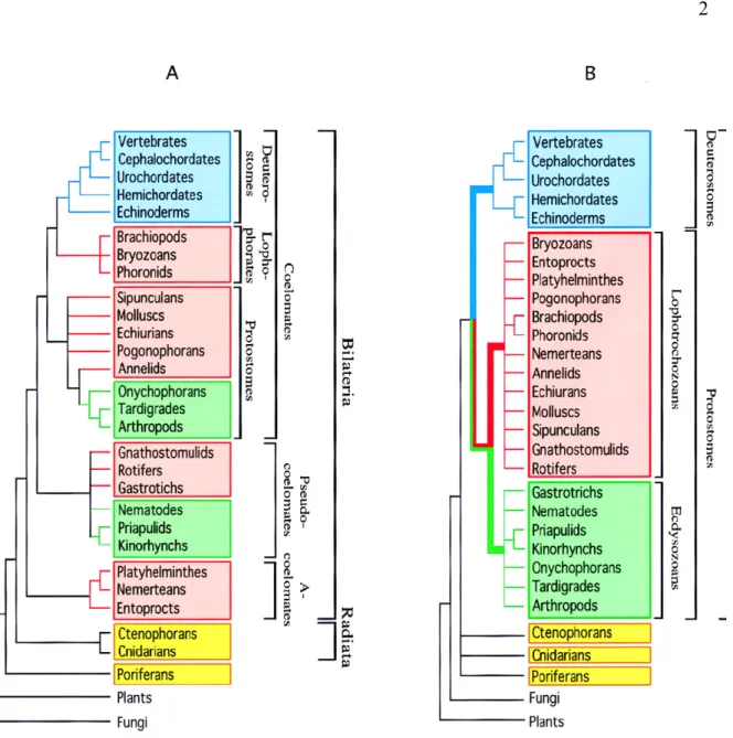
With recent advances of modern molecular technologies, a great amount of molecular datasets (i.e. nucleotide and amino acid sequences) have become available, providing systematists an unprecedented chance to study phylogenies at the molecular level. Molecular phylogenies have confirmed or corrected morphological phylogenies in numerous cases (Adoutte, et al., 2000; Hayasaka, et al., 1996). Figure 1 (Adoutte, et al., 2000) illustrates how molecular phylogeny has changed the classical view of the animal phylogeny.
Figure 1. Metazoan phylogenies.
(A) The traditional phylogeny based on morphology and embryology. (B) The new molecule-based phylogeny.
Adapted from (Adoutte, et al., 2000)
Although molecular phylogeny has achieved great success, with different data and methods, researchers often obtain incongruent phylogenetic results (Delsuc, et al., 2005; Jeffroy, et al., 2006; Philippe, et al., 2005a; Phillips, et al., 2004; Rokas, et al., 2003). Inconsistent phylogenies are mainly caused by systematic and stochastic errors (Phillips, et
al., 2004). During my Ph.D studies, I have been working on heterotachy, one of the causes of systematic errors in phylogenetic inference. In the introduction part of this thesis, I briefly introduce methods for inferring phylogenies, problems in phylogenetic inference and current improvement efforts; thereafter, I focus on heterotachy and current models handling heterotachy.
2 Short introduction to phylogenetic analysis
2.1 Defining a phylogenetic tree
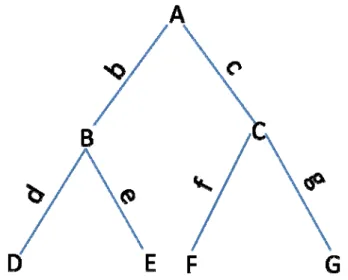
The bifurcating rooted phylogenetic tree presented in Figure 2 consists of seven nodes (species): A, B, C, D, E, F and G; D, E, F and G are leaf nodes, which represent the extant species; A, B, and C are internal nodes, which represent ancestral species and their sequences normally are not available; node A is the common ancestor of all other species. For a general rooted tree with S extant species (leaf nodes), there are a total of 2S-1 nodes and 2S-2 branches.
Figure 2. A bifurcating rooted phylogenetic tree.
Node A has two descendents B and C, such that A’s left node is B, denoting A->left=B; A’s right node is C, denoting A->right=C; B’s branch is b, and C’s branch is c.
The molecular clock hypothesis assumes that substitution rates are constant across lineages. When substitution rates change across lineages, the molecular-clock tree, in which the branch length stands for the evolutionary time, is not valid. In order to reflect variation of substitution rates across lineages, the length of a branch stands for the expected number of substitutions per site (Felsenstein, 2004).
2.2 Alignments
An alignment, which is used to infer a phylogenetic tree, is a set of sequences such that all residues with the same site position (column) are assumed to have originated from a common ancestral residue. Supposing we have S species and N sites, the alignment can be presented as shown:
Species Site 1 Site 2 Site N
Species 1 y11 y12 . . . . . . . . . . . . y1N Species 2 y21 y22 . . . . . . . . . . . . y2N : : : : : : : : Species S yS1 yS2 . . . . . . . . . . . . ySN
2.3 Synapomorphy vs symplesiomorphy
Synapomorphy refers to a derived character state which is shared by a few taxa and is inherited from their last common ancestor. Cladists reconstruct phylogenetic trees based on synapomorphies. Symplesiomorphy, on the other hand, is the derived character state which is shared by a few taxa and is inherited from ancestors older than their last common ancestor. Therefore, a symplesiomorphy does not convey the last ancestor’s information and cannot constitute evidence to infer the phylogenetic relationships. However, symplesiomorphy can impede phylogenetic inference if it is not appropriately handled and is instead interpreted as a synapomorphy.
A B Figure 3. Synapomorphy and symplesiomorphy.
(A) Character state A is a synapomorphy for species 1 and 2. (B) Character state D is a symplesiomorphy for species 2 and 3.
2.4 Phylogenetic artefacts
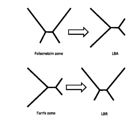
The Long Branch Attraction (LBA) artefact either can group unrelated fast evolving species together during the reconstruction of phylogenetic trees or can lead to overestimations/underestimations of certain branch lengths due to the presence of fast-evolving species. The Felsenstein zone is the area in which two unrelated long branches are always clustered together, and is a special case of the general LBA artefact (Figure 4A ) (Swofford, et al., 2001).
In contrast, Long Branch Repulsion (LBR) is another reconstruction artefact that fails to group two related long branches together during the reconstruction. The Farris zone, which is also referred to as “inverse-Felsenstein” zone (Swofford, et al., 2001), is the area in which two related long branches are always grouped together, and is the positive effect of the LBA artefact. However, the Farris zone could be affected by the LBR artefact (Figure 4B) (Swofford, et al., 2001).
D 1: A 2: D 3: D A 1: A 2: A 3: D D → A D → A
A
B
Figure 4 Felsenstein zone and Farris zone.
(A) An LBA artefact is caused by grouping two unrelated long branches in the Felsenstein zone. (B). An LBR artifact is caused by failing to group two related long branches together in the Farris zone.
2.5 Phylogenetic methods
Three major types of methods have been applied to the reconstruction of molecular phylogenies: maximum parsimony, distance and probabilistic methods. With the advances made in computer technology, researchers are able to use more complicated and computationally intensive models.
2.5.1 Maximum parsimony
The first attempt at molecular phylogenetic analysis is the maximum parsimony method (Camin and Sokal, 1965). Based on the principle of Occam's razor, a phylogenetic tree inferred by the maximum parsimony method has the minimum number of substitutions (Felsenstein, 2004). The initial parsimony methods consider a homogeneous substitution rate along lineages and across sites, yet in real data heterogeneities exist across lineages, sites and time (Jeffroy, et al., 2006; Lartillot, et al., 2007; Philippe, et al., 2003; Yang, 1996b). Alternative maximum parsimony methods have been proposed to improve phylogenetic inference (Farris, 1969; Fitch and Margoliash, 1967; Fitch, 1973; Sankoff and Cedergren, 1983). For instance, weighted parsimony (Sankoff and Cedergren, 1983) tries to distinguish sites by giving them different weights.
However, over long periods of evolutionary time, one site might undergo multiple substitutions, without them being immediately apparent from extant sequences. Sometimes, saturation, in which a site has been substituted more than once and flips back to its original state, can happen. Since maximum parsimony is based on the minimum number of changes, it may not be able to take such situations into account and would assume fewer or even no substitutions for this site. Moreover, for complicated evolutionary patterns found in real data, maximum parsimony methods are only able to allow for some simple model assumptions but not sophisticated ones.
As a result, phylogenetic inference based on the assumption of a minimum number of substitutions would incur systematic errors. Felsenstein (Felsenstein, 1978) demonstrated that parsimony methods are likely to be more inconsistent than maximum likelihoods due to the LBA artefact. On the contrary, it has been shown that maximum parsimony methods perform better than likelihood methods in the Farris zone (Swofford, et al., 2001).
2.5.2 Substitution model based methods
Parsimony methods are essentially a type of non-parametric method, and therefore are not able to allow for explicit evolutionary models. Unlike parsimony methods, model-based methods do not assume that evolution has unfolded with the minimum number of changes; however, they assume that character states are substituted with certain probabilities. One advantage of model-based methods is their allowing for explicit model assumptions.
2.5.2.1 Substitution Matrix Markov process
A first order Markov chain consists of a sequence of variables Xi (i=1,…K), of which the
current state is only dependent on its most immediate previous state, but not dependent on other previous states, such that: 𝑃(𝑋 |𝑋 , 𝑋 , 𝑋 , … , 𝑋 ) = 𝑃(𝑋 |𝑋 ) .
The Markov chain has its state frequency vector λ and transition probabilities P between states. The transition probabilities P can be displayed with a matrix. Supposing there are four states A, B, C and D in a Markov chain, the transition matrix 𝑃 would be:
𝑃 = 𝑃 → 𝑃 → 𝑃 → 𝑃 → 𝑃 → 𝑃 → 𝑃 → 𝑃 → 𝑃 → 𝑃 → 𝑃 → 𝑃 → 𝑃𝑃 →→ 𝑃𝑃 →→ , ∑ 𝑃→ = 1 , (1)
where 𝑃 → stands for the transition probability from state A to B, and 𝑃→ stands for the
probability of A staying at A. If there are two events occurring: transition from state A to state B and from state B to C, then the probability of the two events is 𝑃 → × 𝑃 → . If we don’t know the exact path through which the transitions have been, we can summarize all possible transition events. The probability matrix of substitutions for K events is the product of the matrices P with K times, such that
𝑃𝑟(𝐾) = 𝑃 × 𝑃 × 𝑃 × … × 𝑃 = 𝑃 → 𝑃 → 𝑃 → 𝑃 → 𝑃𝑃 →→ 𝑃𝑃 →→ 𝑃 → 𝑃 → 𝑃 → 𝑃 → 𝑃𝑃 →→ 𝑃𝑃 →→ . (2)
One interesting property of the Markov chain is that after an infinite number of transitions, the state frequency vector λ will be remaining the same. Therefore, λ is also called stationary distribution. Since
𝜆𝑃 = 𝜆 , (3)
λ is the eigenvector of the transition matrix P with the eigenvalue being 1.
In a continuous time Markov chain, the transition events can be modeled with a Poisson distribution (Stewart, 1995). Let 𝜇 be the expected number of events per time unit in a Poisson distribution. Thus, the probability of K events in the Poisson distribution along time 𝑡 is:
𝑓(𝐾 𝑒𝑣𝑒𝑛𝑡𝑠) =( ) ! . (4) Hence, 𝑃𝑟(𝑡), the probability matrix of a Markov chain along time 𝑡, is:
𝑃𝑟(𝑡) = 𝑃 𝑓(𝐾 𝑒𝑣𝑒𝑛𝑡𝑠) = 𝑃 (𝜇𝑡) 𝑒 𝐾!
= 𝑒 ∑ 𝑃 ( )! = 𝑒 𝑒 = 𝑒( ) , (5)
where 𝑃 is the transition matrix, and I is the identity matrix. Let Q=P-I, so
𝑃𝑟(𝑡) = 𝑒 . (6) Q is called the instantaneous rate matrix.
Substitution matrix
The substitution process of molecular data along the phylogenetic tree can be modeled with a continuous time Markov process, thus for the nucleotide sequence with A, C, G, and T states, the transition probability matrix is
𝑃 = 𝑃 → 𝑃 → 𝑃 → 𝑃 → 𝑃 → 𝑃 → 𝑃 → 𝑃 → 𝑃 → 𝑃 → 𝑃 → 𝑃 → 𝑃𝑃 →→ 𝑃𝑃 →→ , (7)
where in the P Matrix, the sum of each row is 1. Since Q=P-I, the sum of each row in the Q matrix is 0. The Q matrix is normalized for the off-diagonal such that the length of the branch stands for the expected number of substitutions per site.
The instantaneous rate matrix Q can be written as:
𝑄 = 𝑅𝛬, (8)
where Λ is a diagonal matrix, and its diagonal values λ1, λ2, λ3, λ4 are the stationary
probabilities of states: 𝛬 = 𝜆 0 0 𝜆 0 0 0 0 0 0 0 0 𝜆 0 0 𝜆 ; (9)
R is the instantaneous rate exchange substitution matrix: 𝑅 = − 𝛼 𝛼 − 𝛽𝛿 𝛾𝜀 𝛽 𝛿 𝛾 𝜀 − 𝜂 𝜂 − . (10)
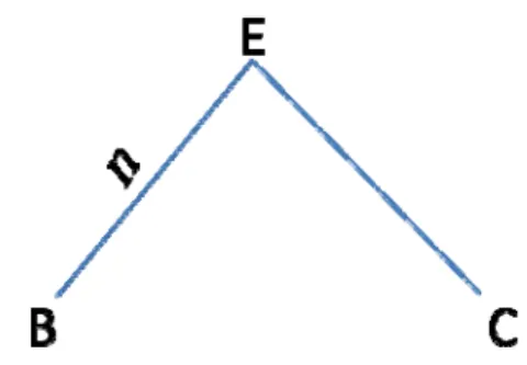
Let species E have two descendent species B and C, and there are n expected substitutions (𝑛 = 𝜇𝑡) occurring from E to B for a given site (Figure 5). According to the equation 6, the probability matrix of the substitutions from species E to species B is:
𝑃𝑟(𝑩|𝑬, 𝑛) = 𝑒 . (11) The exponential of the matrix Q is obtained by diagonalization of the matrix Q (Felsenstein, 2004). The diagonalization of a substitution matrix is a time-consuming process in the likelihood calculation of the phylogenetic tree.
Time reversible model
Most current phylogenetic substitution models are time reversible. Therefore, the probability of being substituted by its descendant state for an ancestral state drawn from the stationary distribution is the same as the one of being substituted by the ancestral state for the descendant state drawn from the stationary distribution (Adachi and Hasegawa, 1996; Felsenstein, 1981; Jones, et al., 1992; Kimura, 1980; Lanave, et al., 1984; Le and Gascuel, 2008; Rodriguez, et al., 1990; Tavare, 1986; Whelan and Goldman, 2001). Supposing an internal state is A and its descendant state is C, we have
𝜆 ∗ 𝑃𝑟(𝐴 → 𝐶) = 𝜆 ∗ 𝑃𝑟(𝐶 → 𝐴). (12) Since 𝑄 = 𝑅𝛬 = − 𝛼 𝜆 𝛼 𝜆 − 𝛽 𝜆 𝛾 𝜆 𝛿 𝜆 𝜀 𝜆 𝛽 𝜆 𝛿 𝜆 𝛾 𝜆 𝜀 𝜆 − 𝜂 𝜆 𝜂 𝜆 − , (13)
when the general time reversible model is assumed, the R matrix will be symmetric, such that α1=α2, β1=β2, γ1=γ2, δ1=δ2, ε1=ε2, η1=η2.
2.5.2.2 Distance methods
Phylogenetic trees can be constructed based on matrices of pair-wise distances among sequences (Fitch and Margoliash, 1967). A straightforward distance was first suggested as simply summarizing the differences between two sequences. Later more sophisticated distances based on substitution models (Jukes and Cantor, 1969; Kimura, 1981) have been used in distance methods. The advantage of model-based distances is that they allow for explicit model assumptions such as multiple substitutions and heterogeneities of substitution probabilities among character states.
Criteria, such as least square (Cavalli-Sforza and Edwards, 1967; Fitch and Margoliash, 1967) and minimum evolution (Kidd and Sgaramella-Zonta, 1971), can be used to infer phylogenetic trees in distance methods. However, searching the optimal tree
with a criterion in a large tree space is a heavy computational task. Using clustering algorithms to infer a phylogenetic tree is much faster than using criteria. Some well-known algorithms include UPGMA (Unweighted Pair Group Method with Arithmetic mean), neighbour joining (Saitou and Nei, 1987), and Bionj (Gascuel, 1997).
Compared with parsimony methods, substitution model based distance methods are more flexible to take heterogeneities of the data into account and correct for the multiple substitutions (Jukes and Cantor, 1969; Kimura, 1980; Tamura and Nei, 1993). However, distance methods using pair-wise sequences fail to recognize the substitutions among the internal nodes, thus consequently the necessary evolutionary information along the whole tree will be lost. Therefore, although distance methods have relative fast computational speeds, they are not optimal for phylogenetic reconstructions (Felsenstein, 2004).
2.5.2.3 Probability based methods
Both maximum likelihood and Bayesian methods involve calculating the likelihoods of the phylogenetic trees, and they belong to the probability based methods.
Likelihood calculation
The likelihood is the probability of the data y given the tree (τ) and parameters 𝜃 of the model. The likelihood function 𝐿(𝜃, 𝜏) is
𝐿(𝜃, 𝜏) = 𝑃𝑟(𝑦|𝜃, 𝜏). (14) Assuming sites 𝑦 , i=1,...N, are independent, 𝑃𝑟(𝑦 |𝜃, 𝜏), the likelihood of the tree (τ) and parameters (θ) over the whole data (y), is the product of the likelihood for each site:
𝑃𝑟(𝑦|𝜃, 𝜏) = ∏ 𝑃𝑟( 𝑦 |𝜃, 𝜏). (15)
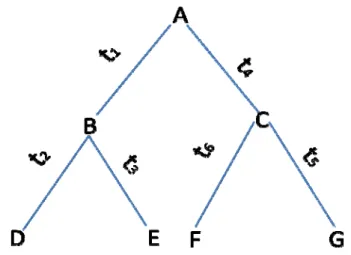
A phylogenetic tree with extant species D, E, F, G and their ancestors A, B, C is shown in Figure 6.
Figure 6. A rooted tree containing six nodes with its root at node A.
Suppose that a site consists of character states for species A, B, C, D, E, F, and G. The likelihood of the tree with branches t1, t2, t3, t4, t5, t6 for this site is
Pr(𝐀, 𝐁, 𝐂, 𝐃, 𝐄, 𝐅, 𝐆|t , t , t , t , t , t , τ)
= Pr(𝐀)Pr(𝐁|t , 𝐀)Pr(𝐃|t , 𝐁)Pr(𝐃)Pr(𝐄|t , 𝐁)Pr(𝐄)Pr(𝐂|t , 𝐀)
Pr(𝐅|t , 𝐂)Pr(𝐅)Pr(𝐆|t , 𝐂)Pr(𝐆) . (16)
The states of external nodes D, E, F and G are observed, so their likelihoods are either 1 or 0 given a specific state s (for DNA data, s∈(A, C, G, T)) . Since the states of the internal nodes A, B and C are unknown, we have to summarize all possible states theses internal nodes: Pr(𝐀, 𝐁, 𝐂, 𝐃, 𝐄, 𝐅, 𝐆|t , t , t , t , t , t , τ) = ∑ ∑ ∑ Pr(𝐀)Pr(𝐁|t , 𝐀)Pr(𝐃|t , 𝐁)Pr(𝐃)Pr(𝐄|t , 𝐁)Pr(𝐄)Pr(𝐂|t , 𝐀) Pr(𝐅|t , 𝐂)Pr(𝐅)Pr(𝐆|t , 𝐂)Pr(𝐆) 𝐂 𝐁 𝐀 . (17)
Here, for 3 internal nodes with the nucleotide data, there are a total of 43=64 combinations of possible internal states. When the number of species increases, the calculation will become tremendous for combining all the possibilities.
Felsenstein thus proposed the pruning algorithm (Felsenstein, 1981) by using the conditional likelihood vector of each node:
Pr(𝐀)Pr(𝐁|t , 𝐀)Pr(𝐃|t , 𝐁)Pr(𝐃)Pr(𝐄|t , 𝐁)Pr(𝐄)Pr(𝐂|t , 𝐀)Pr(𝐅|t , 𝐂)Pr(𝐅)Pr(𝐆|t , 𝐂)Pr(𝐆) 𝐂 𝐁 𝐀 = Pr(𝐀)[ [Pr(𝐃|t , 𝐁)Pr(𝐃)][Pr(𝐄|t , 𝐁)Pr(𝐄)]Pr(𝐁|t , 𝐀)][ Pr(𝐂|t , 𝐀)[Pr(𝐅|t , 𝐂)Pr(𝐅)][Pr(𝐆|t , 𝐂)Pr(𝐆)]] 𝐂 𝐁 𝐀 (18) L𝐁(𝑠) = [Pr(𝐃|t , 𝐁 = 𝑠)Pr(𝐃)][Pr(𝐄|t , 𝐁 = 𝑠)Pr(𝐄)] is the partial likelihood vector for node B conditional on the situation when node B has a character state s.
Hence, the calculation for a tree with three internal nodes is almost equal to calculating 12 combinations of possibilities other than 64. The pruning program greatly saves the computational time and renders likelihood methods feasible for current computational capacities.
Maximum likelihood estimation (MLE)
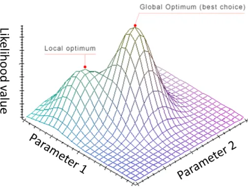
A tree topology with its branch lengths as well as other parameters in the substitution model can be inferred by maximizing the likelihood. However, when the number of parameters increases, the parameter space will become more complicated; and thus the estimate might be more easily stuck into a local maximum, as illustrated in Figure 7.
Figure 7. An illustration of the parameter space.
Tree topologies
The number of possible tree topologies is extremely large in comparison with the number of species (Felsenstein, 2004); moreover, when the topology is changed, the optimal branch lengths will also be changed. Even if the topology is fixed, the change of a single branch length will also influence the optimal lengths of other branches. Considering the huge topology space, the influence of topologies on branch lengths, and irregular likelihood space, the maximum likelihood method confronts a big computational challenge. It is unrealistic for the current computer to explore all the possible topologies in order to infer a phylogenetic tree. One way to overcome this problem is using the Branch and Bound searching algorithm (Hendy and Penny, 1982): initially obtaining a reasonably tree by some heuristic methods (Branch section), then improving the tree by adding more branches (Bound section). One can also attempt to obtain the optimal tree using heuristic searches. For instance, first an initial star decomposition tree is obtained, then branches are added
stepwise and the tree is improved with different methods, e.g. NNI (nearest neighbor interchanging), SPR (Subtree Pruning and Regrafting),TBR (Tree Bisection and reconnection) (Felsenstein, 2004).
Branch lengths and Substitution rates
The branch lengths (b) and instantaneous exchange rate vector 𝜓 ( i.e., α1, β1, γ1, α2,
β2, γ2, in the R matrix) could be optimized by maximizing the likelihood under a fixed
topology. Two major methods have been applied in the current software for maximum likelihood based phylogenetic inference.
Newton-Raphson method
Finding maximum likelihood estimates can be achieved by letting the first derivative of the likelihood be zero. For the maximum likelihood estimate of branch length (b), we have:
= 0. (19)
We can solve this as a root finding problem using the Newton-Raphson method with the first and second derivatives of the likelihood.
Expectation Maximization method
Let 𝑦 be the character state for the extant species (leave nodes), 𝑦 be the character state for the ancestors (internal nodes). So 𝑦 is the observed data and 𝑦 is the unobserved data. In the phylogenetic analyses, we only know the leaves’ states (𝑦), but not the states of any internal nodes (𝑦). In other words, the dataset is incomplete. If 𝑦 was known, then it would be easy to obtain the maximum likelihood estimates of 𝜃 (e.g. the branch lengths as well as the other parameters) in the evolutionary model. One way to handle the incomplete data in the MLE is using an expectation maximization (EM) iterative algorithm (Dempster, et al., 1977). From its name, the EM consists of two steps: expectation and maximization. For instance, Hobolth & Jensen have used the EM to obtain the instantaneous exchange rates (Hobolth and Jensen, 2005).
In the nth iteration of expectation step (E-step), one first estimates G(𝜃; 𝜃 ), the expectation of 𝑓(𝜃; 𝑦) regarding 𝑦:
G(𝜃; 𝜃 ) = 𝐸 | , 𝑓(𝜃; 𝑦), (20)
where 𝑓(𝜃; 𝑦) is the likelihood function in the case of Hobolth’s study, and 𝑦 is obtained conditioned on previous iteration estimation of 𝜃 and y.
In the maximization step (M-step), 𝜃 is obtained by maximizing G(𝜃; 𝜃 ):
𝜃 = argmax G(𝜃; 𝜃 ). (21)
The maximum likelihood estimation of θ is converged, if the difference between 𝜃 and 𝜃 is sufficiently small.
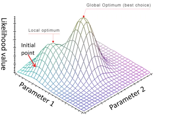
However, if the parameter space is not regular and the initial point we select is close to a local rather than global maximum, the estimations by the Newton-Raphson and EM method could be easily getting stuck at a local maximum (Figure 8). This is because the above methods lack mechanisms to explore the entire parameter space.
Figure 8. An illustration of the local optimum problem.
Convergence to the global maximum depends on a lucky initial point as illustrated for the Newton-Raphson and EM methods.
Simulated annealing via Markov Chain Monte Carlo (MCMC)
When the surface of the parameter space is not regular, simulated annealing via MCMC is more efficient in finding a global maximum in comparison with the Newton-Raphson d and EM methods (Granville, et al., 1994; Kirkpatrick, et al., 1983).
Markov Chain Monte Carlo (MCMC)
Markov Chain Monte Carlo (MCMC) employs random walks along the Markov chain to sample values from probability distributions. In order to get through the barrier to access the desired distribution, Metropolis algorithm is designed to allow accepting non-optimal values with some probabilities (Metropolis, et al., 1953), such that the probability of accepting the proposed 𝜃′ is:
𝛼 = min( ( ) , 1). (22) Here 𝐿(𝜃) refers to the likelihood of 𝜃. One requirement for the Metropolis algorithm is that the transition probabilities from 𝜃′ to 𝜃 and from 𝜃 to 𝜃′ are equal:
𝑃𝑟(𝜃|𝜃 ) = 𝑃𝑟(𝜃 |𝜃). (23) The improved Metropolis-Hasting algorithm allows Markov chain walk through different densities of θ with an adjustment (Chib and Greenberg, 1995; Hastings, 1970), i.e. Hasting ratio ( | )( | ) , so the probability of accepting the proposed 𝜃 is:
𝛼 = min( ( ) ( | )( | ), 1) . (24) Gibbs sampling (Geman and Geman, 1984; Tanner and Wong, 1987) is a special case of the Metropolis-Hasting algorithm. When a series of parameters have to be deduced, it is hard to converge due to the high dimensional parameter space (Tanner and Wong, 1987). Gibbs sampler guarantees a convergence in a multivariate parameter space. The idea behind the Gibbs sampler is that at each iteration, all parameters except one are fixed, and conditioned on these temporarily fixed parameters, the optimal variable parameter can be easily sampled; thus, after a sufficient number of iterations we can achieve the aimed distribution.
Assuming that we have n parameters 𝜃 , 𝜃 , … , 𝜃 , to be sampled, the algorithm of Gibbs sampling is:
For k=1,...m iteration For i=1, ...., n,
𝜽𝒊𝑲~𝜽𝒊|𝜽𝟏𝑲, … 𝜽𝒊 𝟏𝑲, 𝜽𝒊 𝟏𝑲 𝟏, … . 𝜽𝒏𝑲 𝟏, 𝒚
Simulated Annealing via MCMC
The Boltzmann distribution (Costantini and Garibaldi, 1997) describes the energy distribution:
where 𝑃𝑟(𝑖) is the proportion of the molecules being at state i, T is the temperature, ℇ is the energy of state i and K is a constant. When the temperature is high, molecules have high probabilities of being at states with high energy; when the temperature is low, molecules have high probabilities of being at states with low energy. Based on this theory, in the mining industry, the annealing process is preformed to extract crystal from rocks. First, the material is heated to a high temperature, resulting in a high proportion of high energy. Next, the material is gradually cooled down so that the unwanted residues are filtered away (Verhoeven, 1975). This process is iterated for many times until the pure crystals are extracted. The simulated annealing algorithm is inspired by this procedure. One first heats the Markov chain, so the MCMC with high energy is able to traverse the entire parameter surface; and then gradually decreases the temperature, so the MCMC is able to direct itself towards the global maximum and eventually reach it. The probability of accepting new states is:
𝛼 = min( ( ) ( | )( | ), 1), (26)
where 𝑐 is the inverse of the temperature for the nth iteration. There are two kinds of
cooling schedules, one is the linear schedule:
𝑐 = 𝑐 + 𝛽. (27)
The other is the exponential schedule:
𝑐 = 𝑐 × 𝛽. (28)
The choice of the cooling schedule depends on the properties of the dataset.
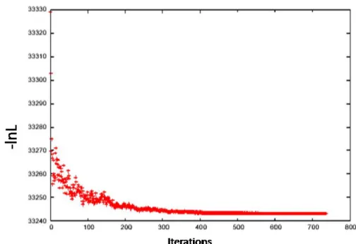
Figure 9 shows that with the temperature dropping down, the MCMC chain eventually gets frozen at the maximal point: the –log likelihood value does not change any more after the 600th iteration.
Figure 9. Plot of the –log likelihood along the MCMC chain in the simulated annealing.
Confidence interval
When the topology is fixed and only branch lengths or the substitution matrix are estimated, the MLE confidence interval can be obtained analytically using the Fisher information (Rice, 1995).
However, when the topology is not fixed, the likelihood surface would be unpredictable and thus the variance of the estimate could not be obtained analytically. One can obtain the variance via resampling of the original dataset. To estimate the variance of the MLE in phylogeny, Felsenstein proposed a non-parametric bootstrap method, which samples sites from the original dataset with replacement to obtain a set of datasets each sharing the same size as the original one (Efron, 1979; Felsenstein, 1985). Theoretically, the variance obtained from the bootstrap should be asymptotically identical to the variance estimated with analytical methods (e.g. using the Fisher information). A consensus tree can be obtained by summarizing all the inference trees from bootstrap with a consensus rule (e.g. strict rule (Rohlf, 1982), majority rule (Margush and McMorris, 1981), semi-strict rules (Bremer, 1990), Nelson rules (Nelson, 1979)). A bootstrap value in a phylogenetic
tree is a probability for two branches to be clustered together given a phylogenetic reconstruction method. Hedges showed that at least 2,000 bootstrap datasets are required to obtain a highly precise result (Hedges, 1992). However, inferring phylogenetic trees from a large amount of bootstrap datasets demands huge computational resources. When several candidate trees need to be compared, we can use the resampling estimated log-likelihood (RELL) method (Kishino, et al., 1990), in which the likelihood of a candidate tree on the bootstrap data is the product of each site’s likelihood of the tree on the original dataset. This approximate method saves a large amount of time to infer other parameters (e.g. branch lengths) of the candidate trees for bootstrap datasets, yet it is reported as robust (Kishino, et al., 1990). However, what we should be aware of is that all bootstrap methods cannot correct the bias of the model (if it exists), and in fact, bootstrap methods only give information of the variance of the phylogenetic inference due to the uncertainty of the data.
Bayesian method
Inferring posterior estimation via MCMC
The maximum likelihood estimation (MLE) tries to find a single optimal value for the parameter of the model given the data. However, Bayesian statisticians argue that parameters of interest have uncertainties given the other unknown parameters as well as the nuisance parameters (Gelman, et al., 2003). Hence, Bayesian statisticians are interested in exploring the parameter space using posterior probabilities.
The Bayes’ theorem gives:
𝑃𝑟(𝜃|𝑦) = ( | ) ( )
∫ ( | ) ( ), (29)
where 𝑦 is the data, θ is the model’s parameter vector of interest. The posterior probability of the model 𝑃𝑟(𝜃|𝑦) is the product of the likelihood 𝑃𝑟(𝑦|𝜃) and the prior 𝑃𝑟(𝜃), and thereafter divided by a normalized factor, which is integrated over all 𝜃.
Computing posterior expectations requires the calculation of high-dimensional integrals, which is often not analytically available. One way is to use the Marko chain
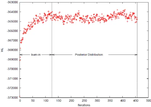
Monte Carlo walking to simulate θ to obtain this integral. Metropolis-Hasting algorithm, which we have introduced in the simulated annealing, is used to construct the MCMC walking. A starting point is randomly picked, and after sufficient number of iterations, the Markov chain would converge to the posterior distribution. When the chain is converged, all the parameters (e.g. branch length, posterior probabilities, etc) should have stable variations, and several independent chains with different random starting points should reach the same area of the parameter estimates. In the MCMC walking, the samples between the starting point and the posterior distribution are referred to as “burn-in” and should be discarded during the analyses (Figure 10).
Figure 10. Plot of the log likelihood along the MCMC chain in the Bayesian analysis.
The posterior estimates of the parameters are the expectations of samples drawn from the posterior distribution. The consensus tree, which consists of the most frequently visited clustering pattern during the MCMC, is the inferred tree of the Bayesian MCMC method.
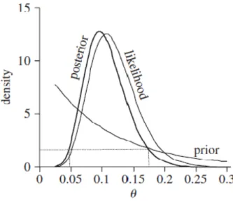
In a Bayesian study, we need to specify a prior distribution for the interested parameter. The prior is a probability distribution which is known or believed a priori. The posterior distribution is a compromise between the likelihood and the prior distribution (Gelman, et al., 2003). If we don’t have strong assumptions about the distribution of the parameters, we normally have a non-informative prior (flat). Figure 11 shows that the posterior distribution is both determined by the likelihood and the prior, which is specified as an exponential distribution with the mean being 0.1.
Figure 11. An illustration of the relationship between likelihood and posterior distribution. Adapted from (Gascuel, 2005)
The prior distribution can be hierarchally controlled with a hyper-parameter. For instance, a parameter x follows a gamma distribution with unknown mean μ, and μ is referred to as the hyper-parameter.
Pros and Cons of the Bayesian MCMC
Bayesian MCMC has recently been gaining popularity in phylogenetic research (Blanquart and Lartillot, 2006; Huelsenbeck and Ronquist, 2001; Huelsenbeck, et al., 2001; Huelsenbeck, et al., 2004; Lartillot and Philippe, 2004; Rodrigue, et al., 2008a; Rodrigue, et al., 2008b; Ronquist and Huelsenbeck, 2003; Smedmark, et al., 2006).
Maximum likelihood estimation (MLE) is almost impossible when it comes to a complicated model with a large number of unknown parameters. In order to estimate the parameters of interest, one needs to integrate over all the other unknown parameters. However, the computation of the integral over a large number of parameters in MLE could be prohibitive. Due to the irregular parameter space, such integration could not be obtained analytically. One advantage of the Bayesian MCMC is that it allows for uncertainties of the parameters of interest due to nuisance parameters, which are not of interest. Supposing that we have parameters θ and v, we are only interested in θ, and v is the nuisance parameter, we have:
𝑃𝑟(𝜃|𝑦) = ∫ 𝑃𝑟(𝜃, 𝑣|𝑦) 𝑑𝑣. (30) This equation can be presented as
𝑃𝑟(𝜃|𝑦) = ∫ 𝑃𝑟(𝜃|𝑣, 𝑦) 𝑃𝑟(𝑣|𝑦)𝑑𝑣. (31) Bayesian MCMC could construct this integration by first drawing v from their posterior distribution, and then drawing θ conditionally on v. With the help of Bayesian MCMC, a number of sophisticated models in phylogenetic inference became possible (Huelsenbeck and Suchard, 2007; Lartillot and Philippe, 2004; Pagel and Meade, 2004).
Furthermore, Bayesian MCMC walk can explore among different model spaces. For instance, the reversible jump mechanism (Green, 1995) allows MCMC to transit between different dimensional spaces. The most frequently visited model would be the optimal model, thus avoiding the model selections in MLE, e.g. likelihood ratio tests (Huelsenbeck, et al., 2004; Pagel and Meade, 2008). This asset makes it possible to infer the phylogenetic tree and evolutionary models simultaneously, thus saving the computational time.
Bayesian MCMC gives uncertainties about parameter estimations, which MLE cannot offer. Although the variations of parameters obtained from the posterior distribution are not the same as the one from the bootstrap process (Yang and Rannala, 2005), the bootstrap is usually not necessary for the Bayesian analyses.
However, prior distributions affect the Bayesian parameter estimation. Yang and Rannala pointed out that estimation of the posterior distribution is sensitive to the branch
lengths’ priors, and misspecification of the priors could incorrectly estimate the posterior probabilities (Yang and Rannala, 2005). Since the prior is very important, the specification of the prior should be practiced carefully.
2.6 Model evaluations
We can compare the fitness among models to see which model best explains the data, and possibly, further explore the nature of the real data, e.g. how species evolve, etc.
2.6.1 Likelihood ratio test
The likelihood value is increased when a model has more parameters. The model is improved when the likelihood value is significantly increased compared with the increase of the number of parameters. When two models to be compared are nested in the framework of the maximum likelihood estimation, likelihood ratio test (LRT) can be used. Suppose 𝜃 is the parameter vector for the model 𝑀 and 𝛩 is the parameter space for 𝜃 . If model 𝑀 is nested in model 𝑀 (𝜃 ∊ 𝛩 , 𝜃 ∊ 𝛩 , 𝛩 ⊂ 𝛩 ), then
( )
( )< 1, (32)
where 𝜃 is the maximum likelihood estimate of 𝜃 for model 𝑀 and 𝐿(𝜃 ) is its likelihood value. It has been shown that the difference between the logarithm of likelihood of model 𝑀 and model 𝑀 asymptotically follows a 𝜒 distribution with 𝑛 degrees of freedom:
𝛥 = 2(ln𝐿 𝜃 − ln𝐿 𝜃 ) ~ 𝜒 (𝑛), (33) where 𝑛 is the difference of the number of parameters between model 𝑀 and model 𝑀 . The null hypothesis assumes model 𝑀 , and the alternative hypothesis assumes model 𝑀 . When the null hypothesis holds, 𝛥 is not significantly large. When model 𝑀 is superior over model 𝑀 , i.e. the extra parameters of the model 𝑀 improve the model fitness considerably, 𝛥 will be significantly large.
In the framework of Bayesian studies, likelihood ratio tests are not valid. However, one can compare two models using the Bayes factor, which is the ratio of two models’ marginal likelihood. Supposing two models M1 and M2, the Bayes factor B12 is defined as
𝐵 = 𝑃𝑟(𝑦|𝑀 ) 𝑃𝑟(𝑦|𝑀 ) =∫ ( | , ) ( | )
∫ ( | , ) ( | ) , (34)
where 𝑃𝑟(𝑦|𝑀 ) is the marginal likelihood for model 𝑀 over all the values of parameter vector 𝜃 , which includes ones in both posterior and non-posterior distribution. If 𝐵 is greater than 1, then M1 is better than M2 for data y; otherwise, M2 is superior over M1.
Bayesian models can be compared using Bayes factor. However, 𝑃𝑟(𝑦|𝑀 ), the integral of the likelihood over the parameters of the model, is difficult to obtain. Several methods have been applied to obtain the integral, nevertheless each method has its own pros and cons.
Bayes factor can also be obtained with the posterior harmonic mean estimator (Newton and Raftery, 1994), which only samples 𝜃 in the posterior distribution, such that
𝑃𝑟(𝑦|𝑀 ) =
( ( | )). (35)
However, it has been shown that harmonic mean estimator tends to over-estimate the marginal likelihood, thus resulting in a higher-dimensional model (Lartillot and Philippe, 2006).
Lartillot and Philippe (Lartillot and Philippe, 2006) applied thermodynamic integration (Gelman and Meng, 1998) for the Bayes factor in phylogenetic cases (Lartillot and Philippe, 2006). Suppose
Z=𝑃𝑟(𝑦|𝑀) = ∫ 𝑃𝑟(𝑦|𝜃, 𝑀) 𝑃𝑟(𝜃|𝑀) 𝑑𝜃. (36) Similar to the thermodynamic system, when heated, the chain is able to move towards all directions and thus explore the entire parameter space; when cooled down, the chain would go towards the posterior distribution. Heating the chain is equal to reducing the weights on
the likelihood, thus the chain is more dependent on the prior and able to explore the entire parameter space with ease; cooling down the chain is equal to putting more weights on the likelihood, thus the chain is moving towards the posterior distribution. Therefore, in order to obtain the integral of the likelihood over the whole parameter space; the chain is running from high temperatures to low temperatures. Let β be a series of continuous numbers from zero to 1: 𝛽 = 0, … . ,1, thus
Z=∫ 𝑃𝑟(𝑦|𝜃, 𝑀) 𝑃𝑟(𝜃|𝑀)𝑑𝛽. (37) Despite the accuracy of this method, the equilibration of the MCMC chain for a series of temperatures in the thermodynamic integration demands a heavy computational time. If 𝑃𝑟(𝑦|𝜃 , 𝑀 )𝑃𝑟(𝜃 |𝑀 ) is normally distributed, Laplace approximation can also be used for the integration (Kass and Raftery, 1995). However, such a requirement (normal distribution) is hard to satisfy for phylogenetic data.
Furthermore, (Schwarz, 1978) proposed the Bayesian Information Criterion (BIC) for the approximation of Bayes factor (see Information criteria below).
2.6.3 Information criteria
When the models under comparison are not nested, one can use information criteria, which give penalties to the likelihood for the increase of the number of parameters.
2.6.3.1 Akaike information criterion (AIC)
Assuming 𝑓(𝑦) is the true distribution of 𝑦, the Kullback-Leibler distance (Bonis and Kullback, 1959; Kullback and Leibler, 1951) gives a true distance between the two distributions 𝑓(𝑦) and 𝑔(𝑦):
𝐼(𝑓; 𝑔) = ∫ ln ( )( ) 𝑓(𝑦)𝑑𝑦. (38) When two models 𝑀 and 𝑀 with their respective parameter vectors 𝜃 and 𝜃 are compared, we have distance between two models:
where ln𝑃𝑟 𝑦 𝜃 is the logarithm likelihood function of 𝜃 , and 𝐸 ln𝑃𝑟 𝑦 𝜃 is the expectation of ln𝑃𝑟 𝑦 𝜃 regarding the data y. However, for model 𝑀 , 𝐸 𝑙𝑜𝑔𝑃𝑟(𝑦|𝜃 ) is not equal to the ln𝑃𝑟 𝑦 𝜃 , where 𝜃 is the maximum likelihood estimate of 𝜃 for a single dataset y. ln𝑃𝑟 𝑦 𝜃 is biased towards overestimation of 𝐸 ln𝑃𝑟(𝑦|𝜃 ), because the data used to infer the 𝜃 are also used to obtain the likelihood value ln𝑃𝑟 𝑦 𝜃 . Akaike deduced that when the number of observations is large enough, the bias is asymptotic to K, the dimensionality of the model (Akaike, 1973):
𝐴𝐼𝐶 = −2ln𝐿(𝜃 ) + 2𝐾. (40)
When the number of observations is small, we could use the corrected AIC (AICc) (Burnham and Anderson, 2002)for model 𝑀 :
𝐴𝐼𝐶 = −2ln𝐿(𝜃 ) + ( ) , (41)
where 𝑁 is the number of the observations.
Although AIC is believed to be asymptotic to the Kullback-Leibler distance, it has been widely reported that AIC prefers higher dimensional models (Hiroshi, 2000).
2.6.3.2 Bayesian information criterion (BIC)
Bayesian information criterion (BIC), which is an approximation of the Bayes factor, is another likelihood penalty method (Schwarz, 1978).
The Bayes factor for two models 𝑀 , 𝑀 is:
𝐵 = ( | )
( | ) , (42)
where 𝑃(𝑦|𝑀 ) is the marginal likelihood of model 𝑀 , and
𝑃𝑟(𝑦|𝑀 ) = ∫ 𝑃𝑟(𝑦|𝑀 )𝑃𝑟( 𝜃 |𝑀 )𝑑𝜃 . (43)
For exponential family distributions, this integration could be approximated using the Laplace method (Davies, 2002):
𝑃𝑟(𝑦|𝑀 ) = −ln𝐿(𝜃 ) + 𝐾ln(𝑁). (44)
Thus BIC can be
We see BIC imposes a harsher penalty to the maximum likelihood estimation than AIC when 𝑁 > 8. Therefore, in general BIC favors a lower dimensional model than AIC (Xiang and Gong, 2005).
2.6.4 Cross validation
As we have introduced, the Kullback-Leibler distance between two models 𝑀 and 𝑀 , with respective parameters 𝜃 and 𝜃 , is:
𝐼(𝜃 ; 𝜃 ) = ∫ ln ( | )( | ) 𝑃𝑟(𝑦|𝜃 )𝑑𝑦 = −(𝐸 ln𝑃𝑟(𝑦|𝜃 ) − 𝐸 ln𝑃𝑟(𝑦|𝜃 )), (46) If we take 𝑀 as the reference model, −𝐸 ln𝑃𝑟(𝑦|𝜃 ) can be the measurement of the fit for model 𝑀 , since for the same dataset 𝐸 ln𝑃𝑟(𝑦|𝜃 ) is always a constant. Hence the cross validation (CV) value for 𝑀 is defined as (Smyth, 2000):
𝐶𝑉 = −𝐸(ln𝑃𝑟 𝑦 𝜃 ) . (47)
As we said, if we use the same dataset to obtain 𝜃 and ln𝑃𝑟(𝑦|𝜃 ), ln𝑃𝑟(𝑦|𝜃 ) will be biased towards overestimation. Therefore, we should use different datasets for estimating 𝜃 and calculating ln𝑃𝑟(𝑦|𝜃 ). However, in real situations, the number of datasets is very limited. So, one solution is to split the data into two partitions. One partition is used as the learning dataset, which is used to infer the parameters of 𝜃 , and the other partition is the testing dataset, which is used to compute ln𝑃𝑟 𝑦 𝜃 . In order to obtain the expectation of ln𝑃𝑟 𝑦 𝜃 , the same dataset can be reused several times by being split into different random partitions. There are several ways to split the data. N-fold is one way to split the dataset: divide the data into N parts, each time, take one part as the learning dataset, and take the rest of the dataset (N-1) parts as the testing dataset. Compared with AIC and BIC, CV is more accurate (Smyth, 2000), however, it takes more computational time.
2.6.5 Posterior predictive test 2.6.5.1 Posterior predictive data
Posterior predictive data 𝑦 are simulated with the parameters drawn from the posterior distribution for data y and model M, such that the distribution of 𝑦 is:
𝑃𝑟(𝑦 |𝑦, 𝑀) = 𝑃𝑟(𝑦 |𝜃, 𝑦)𝑃𝑟(𝜃|𝑦, 𝑀)𝑑𝜃
= ∫ 𝑃𝑟(𝑦 |𝜃)𝑃𝑟(𝜃|𝑦, 𝑀)𝑑𝜃. (48) The second line of equation 48 shows that the posterior predictive data 𝑦 and the real data 𝑦 are independently conditional on 𝜃. If the model accurately reflects the real data, then the posterior predictive dataset would be virtually identical to the real data. Based on this assumption, one can examine the similarity between the posterior predictive dataset and the original dataset (Gelman, et al., 2003) using different statistics. For instance, mean diversity is the mean of the number of observed states per column (site), and can be used to check the similarity between the posterior predictive data and the real data (Lartillot, et al., 2007).
2.6.5.2 Posterior predictive test
Posterior predictive discrepancy tests use generalized parameter-dependent statistics. I will first introduce classical statistical tests, and then posterior predictive discrepancy tests using parameter-dependent test statistics.
Model assessment using classical statistics
Model assessments can be performed using classical statistical tests, such as the χ2 test for a contingency table, the χ2 goodness-of-fit test, etc. Let T(y) denote a test statistic. For the χ2 test, we have:
𝑇(𝑦) = ∑ ( ) , (49) where 𝑂 is the observed value, 𝐸 is the value expected by the model. In the null hypothesis 𝐻 , ∑ ( ) follows a 𝜒 distribution with N-R degrees of freedom and R is the reduction in the degree of freedom. If the model is significantly far from the real data,
then ∑ ( ) will be large. Let the p value of the test statistic 𝑇 be the tail probability. The test then is constructed as
𝑝(𝑦) = 𝑃𝑟(𝑇(𝑌) ≥ 𝑇(𝑦)|𝐻 ) , (50)
where data Y are under the null hypothesis, y is the observed data. In the case of our example, 𝑇(𝑌) follows a 𝜒 distribution. In the classical statistic test, we only need to calculate 𝑇(𝑦), then we can locate 𝑇(𝑦) in the distribution of 𝑇(𝑌) with a 𝜒 table. In the context of MLE, the statistic 𝑇(𝑦) does not depend on any unknown parameters and is well defined, since all the parameters have already been inferred by maximizing the likelihood.
Posterior predictive assessment using discrepancy
Posterior predictive tests can be used to assess Bayesian models, which classical test statistics cannot be applied to.
In order to perform the model assessment using a test statistic, the null distribution should be known a priori. However, sometimes, due to the existence of nuisance parameters υ, the statistic 𝑇 is parameter-dependent. Moreover, in the context of the Bayesian study, the parameter estimations are obtained by marginalizing over the posterior distribution. Therefore, the test statistic T is parameter dependent, and thus its null distribution is difficult to estimate. Furthermore, due to the small size of the dataset, or irregular parameter space, the null distribution of the statistic is not easily obtained in most cases.
One solution is to make simulations of the null distribution. However, due to the presence of unknown nuisance parameters in the model, simulation of the null distribution is difficult. Since posterior predictive data 𝑦 |(𝑀, 𝑦) are generated based on the posterior distribution of the model M, the posterior predictive data already consider the nuisance parameters and the priors of the parameters. Therefore, Rubin proposed using the posterior predictive distribution as the reference (Null) distribution for testing the null hypothesis model 𝐻 (Rubin, 1984). Gelman et.al, used a discrepancy D(y,φ) to denote the parameter-dependent statistic, and generalized the classical statistical assessments with posterior
predictive discrepancy tests (Gelman, et al., 1996). The key to the posterior predictive discrepancy test is using the posterior predictive distribution as a null distribution. The p value for the posterior predictive test is:
𝑝(𝑦 |𝑦 ) = ∫ ∫ 𝑃𝑟(𝐷(𝑦 ) ≥ 𝐷(𝑦 )|𝜃, 𝜐)𝑃𝑟(𝜃, 𝜐|𝑦 , 𝐻 )𝑑𝜃𝑑𝜐. (51) The posterior predictive p value can be directly obtained by counting the frequency. Similar to the p value of a classical statistical test, a low posterior predictive p value suggests a low risk if we reject the model under the null hypothesis.
The generalized parameter-dependent statistics are no longer restricted to the MLE context and can be used for any applications, such as goodness of fit tests, likelihood ratio tests (LRT) (Protassov, et al., 2002), etc.
2.7 Data
Nucleotide sequences are three times longer than amino acid sequences if they contain the entire protein-coding information. Nevertheless, the computational time used for inferring phylogenetic trees with nucleotide sequences is much less than the one with amino acid sequences given a small substitution matrix [4×4] for nucleotides and a large substitution matrix [20×20] for amino acids, since the computational time largely depends on the size of the matrix. However, the nucleotide data with four characters have a higher chance than the amino acid data of experiencing multiple substitutions and saturation, which might impede phylogenetic inference.
Nevertheless, phylogenetic analyses of amino acid data also have their own problems. For instance, synonymous substitutions, which change the nucleotide character but do not change the character of amino acid, also contain phylogenetic information (Muse and Gaut, 1994). Thus, using amino acid data might truncate the necessary phylogenetic signals. Recently, researchers developed codon models, in which every three nucleotides are transformed into one codon state; in total there are 61 codon states in the codon model (Goldman and Yang, 1994; Muse and Gaut, 1994). As a result, codon models dramatically increase the computational time considering the large size of the substitution matrix
[61×61], but are biologically more realistic and should be preferred (Ren, et al., 2005; Whelan, 2008). The choice of the data type is the consequence of a tradeoff among computational time, phylogenetic signals, and the biological reasoning.
3 Challenges of
inferring phylogeny and their solutions
Most inconsistent phylogenies result from either stochastic or systematic errors. Other reasons causing incorrect phylogenies include erroneously interpreting paralogous genes as orthologous data, or taking genes affected by horizontal gene transfer (HGT) events, etc. In this section, only stochastic and systematic errors will be introduced.
3.1 Stochastic errors
When a dataset is not large enough, stochastic noise may overwhelm the genuine phylogenetic signal and thus reduces the resolution of phylogenetic inference or causes stochastic errors. One major outcome of the stochastic error is that nodes in the tree cannot be completely resolved with low statistical supports (e.g. low bootstrap values). One way to reduce the stochastic error is to employ a large scale dataset (Eisen, 1998; Philippe and Telford, 2006) assuming that a dataset with an infinite number of sites would eventually receive 100% statistical support. For instance, 106 genes, which are distributed throughout all 16 chromosomes of Saccharomyces.cerevisiae genome and represent about 1% of the genomic sequence, are used to establish the phylogenetic tree of the genus Saccharomyces (Rokas, et al., 2003). The separate analyses of these 106 genes yield 20 different phylogenetic trees, among which 6 topologies receive strong bootstrap (>70%). In contrast, the concatenated data with all the 106 genes receive a 100% bootstrap support (Rokas, et al., 2003). Thus it was concluded that the stochastic errors have been largely diminished by the concatenation of the data.